Synthesis of observed air–sea CO<sub>2</sub> exchange fluxes in the river-dominated East China Sea and improved estimates of annual and seasonal net mean fluxes

(1)

BGD

10, 13977–14007, 2013

Synthesis of observed air–sea CO2 exchange fluxes

C.-M. Tseng et al.

Title Page

Abstract Introduction

Conclusions References

Tables Figures

◭ ◮

Back Close

Full Screen / Esc

Printer-friendly Version Interactive Discussion

Discussion

P

a

per

|

Dis

cussion

P

a

per

|

Discussion

P

a

per

|

Discussio

n

P

a

per

|

Biogeosciences Discuss., 10, 13977–14007, 2013 www.biogeosciences-discuss.net/10/13977/2013/ doi:10.5194/bgd-10-13977-2013

Open Access

Biogeosciences

Discussions

Geoscientiic Geoscientiic

This discussion paper is/has been under review for the journal Biogeosciences (BG). Please refer to the corresponding final paper in BG if available.

Synthesis of observed air–sea CO

2

exchange fluxes in the river-dominated

East China Sea and improved estimates

of annual and seasonal net mean fluxes

C.-M. Tseng1, P.-Y. Shen1, and K.-K. Liu2

1

Institute of Oceanography, National Taiwan University, Taipei 106, Taiwan

2

Institute of Hydrological & Oceanic Sciences, National Central University, Jungli, Taoyuan 320, Taiwan

Received: 3 July 2013 – Accepted: 12 August 2013 – Published: 26 August 2013

Correspondence to: C.-M. Tseng (cmtseng99@ntu.edu.tw)

(2)

BGD

10, 13977–14007, 2013

C.-M. Tseng et al.

Title Page

Tables Figures

◭ ◮

Back Close

Full Screen / Esc

Discussion

P

a

per

|

Dis

cussion

P

a

per

|

Discussion

P

a

per

|

Discussio

n

P

a

per

|

Abstract

Limited observations exist for reliable assessment of annual CO2 uptake that takes

into consideration the strong seasonal variation in the river-dominated East China Sea (ECS). Here we explore seasonally representative CO₂ uptakes by the whole East China Sea derived from observations over a 14 yr period. We firstly identified the

bi-5

ological sequestration of CO2 taking place in the highly productive, nutrient-enriched

Changjiang river plume, dictated by the Changjiang river discharge in warm seasons. We have therefore established an empirical algorithm as a function of sea surface temperature (SST) and Changjiang river discharge (CRD) for predicting sea surface

pCO₂. Synthesis based on both observation and model show that the annually

av-10

eraged CO₂ uptake from atmosphere during 1998–2011 was constrained to about 1.9 mol C m−2yr−1. This assessment of annual CO2 uptake is more reliable and

rep-resentative, compared to previous estimates, in terms of temporal and spatial cover-age. Additionally, the CO₂time-series, exhibiting distinct seasonal pattern, gives mean fluxes of−3.0, −1.0, −0.9 and−2.5 mol C m−2yr−1 in spring, summer, fall and winter,

15

respectively, and also reveals apparent inter-annual variations. The flux seasonality shows a strong sink in spring and a weak source in late summer-early fall. The weak sink status during warm periods in summer-fall is fairly sensitive to changes ofpCO₂ and may easily shift from a sink to a source altered by environmental changes under climate change and anthropogenic forcing.

20

1 Introduction

Continental shelves generally receive large loads of carbon from land on the one hand and sustain rapid biological growth and biogeochemical cycling with rates much higher than those in the open ocean, on the other hand (Walsh, 1991). Despite their rel-atively small total surface area (∼8 % of the whole ocean area), they overall play

25

(3)

BGD

10, 13977–14007, 2013

C.-M. Tseng et al.

Title Page

Tables Figures

◭ ◮

Back Close

Full Screen / Esc

Discussion

P

a

per

|

Dis

cussion

P

a

per

|

Discussion

P

a

per

|

Discussio

n

P

a

per

|

CO2(0.2∼0.5 Gt C yr− 1

), which represents 10∼30 % of the current estimate of global

oceanic CO2 uptake (Borges et al., 2005; Cai et al., 2006; Chen and Borges, 2009;

Laruelle et al., 2010). In addition, the coastal seawaters interact and exchange strongly in complex ways with the atmosphere, and the open ocean. Thus, the environment complexities and diversity of the shelf seas pose a challenge to characterization of the

5

dynamic carbon cycling in these regions. Based on literature compilations and global extrapolation in estimates of CO2sequestration in marginal seas, the aforementioned

estimates existed with large uncertainties. That is because many regions are grossly under-sampled, especially the mid-latitude continental shelves (Borge et al., 2010).

It was reported continental shelves at mid- and high-latitudes generally act as a sink

10

for atmospheric CO2, while as a source of CO2at low latitudes, between 30◦S–30◦N.

The East China Sea (ECS) is situated between the low- and mid-latitudes (between 25◦N–34◦N) with estimated overall CO2 sink strength of 1∼3 mol C m−

2

yr−1 (Peng, et al., 1999; Tsunogai et al., 1999; Wang et al., 2000; Shim et al., 2007; Zhai and Dai, 2009; Tseng et al., 2011). As a whole, the ECS (∼0.2 % of global ocean area) could

15

yield annual carbon uptake of 0.01∼0.03 Gt C, representing 0.5∼2.0 % of the global

uptake. This implies a relatively high CO2uptake rate compared to other ocean regions.

Previously reported air–sea CO₂ fluxes were, however, biased by inadequate spatial and/or temporal coverage. For instance, Tsunogai et al. (1999) first showed estimates of∼3 mol C m−2yr−1uptake of the ECS from atmospheric CO2based on extrapolating

20

from a single transect data of the PN line across the central ECS. Other later CO₂flux studies in the ECS with uptake rates of 1∼3 mol C m−2yr−1had been spatially limited

as well (Fig. 1a). Moreover, a reliable quantification in seasonally representative CO2

uptakes by the whole ECS has not been established to date.

The observational requirements to adequately investigate air–sea CO₂ exchange

25

(4)

produc-BGD

10, 13977–14007, 2013

C.-M. Tseng et al.

Title Page

Tables Figures

◭ ◮

Back Close

Full Screen / Esc

Discussion

P

a

per

|

Dis

cussion

P

a

per

|

Discussion

P

a

per

|

Discussio

n

P

a

per

|

tion/respiration, surface/subsurface sea waters and river waters. The dominant pro-cesses in the ECS vary by seasons and regions, with typically active biological uptake of CO2 in warm periods and intensely physical mixing and solubility of CO2 in the

cold seasons (Tseng et al., 2011; Chou et al., 2011). In addition, pCO_2w distribution is subjected to mixing of varied water masses which are characterized by the

nutrient-5

rich and less saline Changjiang Diluted water (CDW, waters within 31 – isohaline) and warm, saline and nutrient-depleted Kuroshio (KW), shelf mixed (SMW) and Taiwan Warm Current (TWC) waters (Fig. 1b). Consequently, the mixing of water masses with different biogeochemical characteristics in the ECS causes the spatial/temporal CO2

variations (e.g., Tseng et al., 2011). Further, various circulation regimes lead to the

10

shelf-edge processes for material exchange between the East China Sea Shelf and the adjoining Kuroshio (e.g., Liu et al., 2010). Thus, to enable better quantification of the ECS CO2uptake capacity reiterates the need of greater spatial and temporal

reso-lutions in observational data, which are needed for accurate estimation of air–sea CO₂ fluxes in the ECS over an annual cycle.

15

This study presents new data and expands on the approach of Tseng et al. (2011) of adopting innovative methods to extend the spatial and temporal coverage for broad scale assessments of distribution and air–sea exchange fluxes of CO2. A regional

syn-thesis based on satellite remote sensing data (e.g., sea surface temperature, SST) calibrated with direct near surface underway pCO₂ measurements and modified by

20

the Changjiang (a.k. a Yangtze) river discharge (CRD) has therefore been established. The CRD as the dominant freshening nutrient source of the ECS played a key influ-ence on modulating the CO₂uptake (Tseng et al., 2011). We found firstly an empirical relationship for predicting water pCO2 as a function of CRD and SST. The relation

was then applied to the whole ECS shelf (25–33.5◦N and 122–129◦E) after the model

25

generatedpCO_2w results had been well validated against the observed pCO_2w. The resultant algorithm aimed to improve the quantification of shelf CO2uptake capacity in

(5)

BGD

10, 13977–14007, 2013

C.-M. Tseng et al.

Title Page

Tables Figures

◭ ◮

Back Close

Full Screen / Esc

Discussion

P

a

per

|

Dis

cussion

P

a

per

|

Discussion

P

a

per

|

Discussio

n

P

a

per

|

to 2011 that yield an annual mean value of unsurpassed accuracy after an examination of di_fferent gas-transfer algorithms.

2 Materials and methods

2.1 Analytical methods and data analyses

Twelve seasonal cruises for direct underway atmospheric (pCO2a) and water pCO2

5

(pCO_2w) with hydrographic measurements were carried out in the East China Sea (ECS) shelf (25–32◦N and 120–128◦E) between June 2003 and July 2011 on board

R/V Ocean Researcher I.There was also one earlier cruise in July 1998 performing

similar measurements. Most cruises (n=9) were conducted in warm seasons that al-lowed delineation of the effects of discharge variations on the CO2 uptake, whereas

10

there were also cruises conducted in each of the other seasons (spring, fall and win-ter). Additional data were obtained to provide the complete seasonal coverage of CO₂ distribution in the ECS.

The cruise tracks and hydrographic stations superimposed on main surface currents in this study area are shown in Fig. 1b. The underway system with continuous flow

equi-15

libration, provided by the National Oceanic and Atmospheric Administration (NOAA) of the United States, is fully automated and uses gas standards (the xCO2 of the

four standards was 266.56, 301.76, 406.72, and 451.37 ppm, respectively) from NOAA (Wanninkhof, 1993). Precision and accuracy achieved with this method are±0.1 and ±2 µatm, respectively. The distributions of sea surface salinity (SSS) and temperature

20

(SST) were recorded using a SBE21 SEACAT thermosalinograph system (Sea-Bird Electronics Inc.). Surface chlorophylla(chla) concentration was measured with a Sea Tech fluorometer attached to the SeaBird CTD for a continuous in-vivo fluorescence, with data calibrated by in-vitro fluorometry (Turner Design 10-AU-005). Nutrient (e.g., nitrate₊nitrite) and chlaconcentrations were measured according to Gong et al. (1996)

25

(6)

BGD

10, 13977–14007, 2013

C.-M. Tseng et al.

Title Page

Tables Figures

◭ ◮

Back Close

Full Screen / Esc

Discussion

P

a

per

|

Dis

cussion

P

a

per

|

Discussion

P

a

per

|

Discussio

n

P

a

per

|

The time-series records including remotely sensed SST data, archived hydrographic salinity (Japan Oceanographic Data Center, JODC), wind speed (at PenGaYi Islet; 25.62◦N, 122.07◦ E), Changjiang river discharge (CRD, Datong hydrological gauge station; 30.76◦ N, 117.62◦ E) and air pCO₂ data (JeJu Island, South Korea; 33.28◦ N, 126.15◦E) for estimatingpCO2w with related air–sea exchange flux in the ECS

re-5

gion (25–33.5◦N and 122–129◦E) were briefly described as below. The weekly av-erage SST data were derived from the Advanced Very-High Resolution Radiometer (AVHRR) images from the NOAA with 1 km×1 km resolution (http://www.osdpd.noaa.

gov/ml/ocean/sst.html). The AVHRR-SST agreed well with ship-board observations (Tseng et al., 2007, 2009a, b). The archived hydrographic salinity data in the ECS

10

were provided by Japan Oceanographic Data Center (JODC) with data resolution of 1◦×1◦ grids (http://jdoss1.jodc.go.jp/cgi-bin/1997/bss). The monthly wind speed data

were estimated from the daily average data at land-based weather station of PenGaYi Islet (25.62◦_{N, 122.07}◦_{E) in the ECS provided by the Taiwan Central Weather}

Bu-reau (TCWB). The monthly CRD data at Datong hydrological gauge station (30.76◦N,

15

117.62◦E) in the lower reach of Changjing were obtained from the Hydrological infor-mation Centre of China. The air pCO₂ was estimated from the monthly atmospheric

xCO2(mole fraction) measured at JeJu Island (South Korea; 33.28◦ N, 126.15◦E),

af-ter correction for waaf-ter vapor pressure at 100 % humidity with SST and salinity data (http://www.esrl.noaa.gov/gmd/ccgg/globalview/).

20

2.2 Air-sea CO2exchange flux estimates

Air–sea exchange flux,F, of pCO2 is estimated using the equation: F =K×δpCO2,

whereK (gas transfer coefficient)=kL(k: transfer velocity;L: gas solubility),δpCO2

is the di_fference between thepCO₂of surface water and air (i.e.,pCO_2w−pCO2a). The

pCO2a was estimated from the monthly averagepCO2observed at JeJu Island during

25

the study period. Solubility of CO2as a function of water temperature and salinity can

(7)

BGD

10, 13977–14007, 2013

C.-M. Tseng et al.

Title Page

Tables Figures

◭ ◮

Back Close

Full Screen / Esc

Discussion

P

a

per

|

Dis

cussion

P

a

per

|

Discussion

P

a

per

|

Discussio

n

P

a

per

|

relationship:k=0.31×u2×(Sc/660)−0.5, where Schmit number (Sc) is

temperature-dependant for CO2 in seawater, computed from in situ temperature data anduis the

wind speed at 10 m height obtained from PenGaYi station (monthly average wind data from the TCWB database of 1998–2011). The parameterization of Wanninkhof (1992), representing a reasonable estimate for calculating wind-inducedk, was firstly used for

5

comparison with previous flux estimates in the ECS. Then, the air–sea exchange fluxes of CO2in the ECS reported in the previous studies were re-calculated according to the

consistent wind speed data and Wanninkhof’s algorithm used in this study. Finally, un-certainties of CO₂fluxes due to using di_fferent gas-transfer algorithms (e.g., Liss and Merlivat, 1986; Wanninkhof, 1992; Wanninkhof and McGillis, 1999; Jacobs et al., 1999;

10

Nightingale et al., 2000; McGillis et al., 2004; Ho et al., 2006; Wanninkhof et al., 2009) and their appropriate flux ranges in the ECS shelf were quantitatively evaluated.

2.3 Areal mean ofpCO2and environmental variables

To obtain a representative mean value for the ECS shelf, we prepared the interpolated data set of 0.01◦×0.01◦(about 1 km×1 km) grid points from observedpCO2and other

15

environmental variables (e.g., SST, Salinity, N₊N, chlaetc.) by kriging and then calcu-lated the areal means by integrating over the survey area. The grid resolution matches the spatial resolution of weekly AVHRR-SST data. For the areal mean of the air–sea flux, we first calculated the flux within a given grid box along the cruise track for under-waypCO2measurement using the average values of SST, salinity, and δpCO2 in the

20

box and the monthly average wind speed; then, we calculated the areal mean CO2flux

(8)

BGD

10, 13977–14007, 2013

C.-M. Tseng et al.

Title Page

Tables Figures

◭ ◮

Back Close

Full Screen / Esc

Discussion

P

a

per

|

Dis

cussion

P

a

per

|

Discussion

P

a

per

|

Discussio

n

P

a

per

|

3 Results and discussion

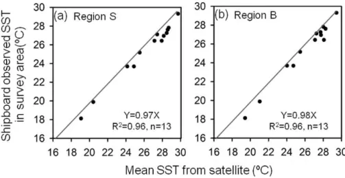
3.1 Representativeness of the study region

The East China Sea (ECS) is a large marginal sea (25–33.5◦_{N, 120–129.5}◦_{E) in the}

northwestern Pacific with an area of∼0.6×106km2, of which 3/4 is a wide continental

shelf (Fig. 1a). Our cruise region is situated in the southern and western ECS, covering

5

an area about a half of the whole ECS. In order to evaluate whether the cruise data are representative of the entire ECS, we compared the areal mean values of AVHRR-SST from the two model areas against the observed average AVHRR-SST data. The two areas are respectively a small one (Region S, 25–31.5◦_{N and 123–126}◦_{E), which is similar}

to the cruise survey area and a bigger one (Region B, 25–33.5◦N and 122–129◦E),

10

which covers almost the whole ECS (Fig. 1a). Briefly, the areal mean SST calculated from observed values in cruise survey area correlated well with the average AVHRR-SST data in two model domains with perfect regression relationships (R2=0.96) as shown respectively in Fig. 2a and b. It indicates, on the one hand, the remotely sensed SST data used here are reliable and validated in terms of data assurance; on the other

15

hand, the areal mean SST data obtained on our cruise investigations can represent the variability of the areal mean value of the entire ECS. Therefore, it is reasonable to assume that the relationship between the areal means ofpCO₂ and mean values of hydrographic variables obtained on our cruises was also representative for the entire ECS. Further, we may use the aforementioned relationship to derive representative

20

average values ofpCO₂for Region B, which should be the most representative for the ECS shelf.

3.2 Summer CO2uptake determined by Changjiang river discharge

Figure 1c and d shows the composite distributions of pCO2w and air–sea CO2

ex-change flux from nine cruises in summer between 2003 and 2011. As reported

pre-25

(9)

BGD

10, 13977–14007, 2013

C.-M. Tseng et al.

Title Page

Tables Figures

◭ ◮

Back Close

Full Screen / Esc

Discussion

P

a

per

|

Dis

cussion

P

a

per

|

Discussion

P

a

per

|

Discussio

n

P

a

per

|

variations of water masses (Tseng et al., 2011). LowerpCO_2wvalues were observed in the CDW plume area near the Changjiang river mouth and higher values in the south-eastern shelf area, where saline and nutrient-depleted Kuroshio, Shelf Mixed Water and Taiwan Warm Current Water prevailed. Also, the distribution of CO₂ flux in the ECS resembled that ofpCO2. More negative values (i.e., uptake of atmospheric CO2

5

by surface water) were mostly found in the nutrient-rich river plume area with a gradual increase to the east and south. Despite the high sea surface temperature in summer that favored release of CO2 to the atmosphere, the Changjiang river plume acted as

a strong CO2 sink, mainly due to CO2 drawdown in the outflow region where

river-ine nutrients induced strong phytoplankton growth, resulting in high chlaand reduced

10

pCO₂in the surface layer (Tseng et al., 2011). In addition, the CO₂distribution/uptake dynamics were yearly associated with the changes of the plume expansion determined by the CRD:

pCO₂=−4.1×CRD+527.6, R2=0.96; (1)

CO2flux=−0.21×CRD+7.9, R2=0.97,n=8. (2)

15

where CRD is in units of 103m3s−1. The results further demonstrate Changjiang river discharge governs coastal ocean production and CO2 uptake capacity in the East

China Sea shelf in summer.

3.3 Empirical algorithm to simulate seasonalpCO2wvariations 20

To derive representative mean values ofpCO2w in different seasons in the entire ECS

shelf, we may use the strong correlation between river discharge and CO2uptake

men-tioned above (e.g., Tseng et al., 2011). We thus developed an empirical algorithm by using the monthly areal mean (referred to as “average” hereafter) of observedpCO2w,

and SST and the CRD during warm periods. The data mentioned above were collected

25

during warm cruises from May to November between 1998 and 2011. Firstly, we found normalizedpCO₂at 25◦_{C (N}_p_CO

2) correlated negatively with the CRD (×10 3

m3s−1

(10)

BGD

10, 13977–14007, 2013

C.-M. Tseng et al.

Title Page

Tables Figures

◭ ◮

Back Close

Full Screen / Esc

Discussion

P

a

per

|

Dis

cussion

P

a

per

|

Discussion

P

a

per

|

Discussio

n

P

a

per

|

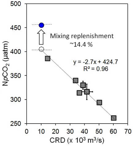
with a good regression relationship (Fig. 3) as follows:

NpCO2at 25◦C=−2.7×CRD+424.7 (R2=0.96) (3)

Here, NpCO2at 25◦C, which is the observed averagepCO2wnormalized to a constant

temperature of 25◦_{C (mean SST of all cruises), was computed by using the following}

equation proposed by Takahashi et al. (1993).

5

NpCO2atTmean=(pCO2w)obs×exp[0.0423(Tmean−Tobs)] (4)

whereTmeanis 25◦C andTobs is the observed monthly mean values and (pCO2w)obsis

the observed averagepCO2w. The purpose of “pCO2 normalized to 25◦C” is to

elim-inate the temperature effect in order to discern other factors (e.g., biological activities, air–sea exchange and vertical transport of subsurface waters etc.) that affectpCO2.

10

The inversely linear relationship between the NpCO2and CRD during warm periods

as shown by Eq. (1) indicates thatpCO_2wchanges in the ECS shelf water were mainly governed by biological processes, while other processes, such as the upward trans-port of dissolved inorganic carbon (DIC) from subsurface waters and the air–sea CO2

exchange, are minimal under strong stratification.

15

We finally refined the empirical algorithm for predictingpCO_2waccording to Eqs. (3) and (4) as below:

pCO2w=(−2.7×CRD+424.7)×e[0.0423×(Tobs−25)] (5)

where −2.7 is the slope obtained from the plot of NpCO2 vs. CRD; CRD is the

Changjing river discharge in units of 103m3s−1;Tobs is the monthly average

AVHRR-20

SST.

However, when we applied the same relationship to the cold season, we found that the relationship underestimated the NpCO2 (Fig. 3). The extra increment was

proba-bly mainly caused by the increase in DIC provided by enhanced vertical mixing in the cold season. It is necessary to compensate for the mixing e_ffect in the equation. As

(11)

BGD

10, 13977–14007, 2013

C.-M. Tseng et al.

Title Page

Tables Figures

◭ ◮

Back Close

Full Screen / Esc

Discussion

P

a

per

|

Dis

cussion

P

a

per

|

Discussion

P

a

per

|

Discussio

n

P

a

per

|

shown in Fig. 3, an increase of 57.4 µatm was needed to reach the observed NpCO₂of 455.1 µatm for January from the computed NpCO2 of 397.7 µatm, which was

calcu-lated from the CRD of 10 211 m3s−1. This increment represents a 14.4 % increase to account for the mixing replenishment. For the model calculation, the seasonal mixing contribution could be estimated from the data of wind speed (W) and remotely sensed

5

SST (T) through the relationship between the mixing ratio and the mixing index de-fined asW/T (see Figs. S1–S3 in Supplement materials). An enhancement factor of ca. 14.4 % could be, for instance, applied to account for the strongly vertical mixing in the months of January, February and March, when the SST was the lowest and wind speed highest during northeast monsoon. About 11.8, 8.9 and 2.4 % of the mixing

ra-10

tios due to gentle mixing were for December, April and November, respectively, when the SST was higher and wind speed lower.

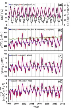
3.4 Time-series of model results vs. field observations

The 14 yr time-series of model results of monthly meanpCO2w,δpCO2 and the air–

sea CO₂ flux in Regions S and B over the study period (1998–2011) are shown in

15

Fig. 4, in which mean observed values of the 13 cruises are also plotted for compar-ison. It is clear that all modeledpCO2w,δpCO2 and the CO2 flux agree well with the

observations (Figs. 4 and S4). As shown, the time-series (Fig. 4b) is characterized by a distinct seasonal pattern with a maximum in late summer-early fall and a minimum in spring. In general, thepCO2w mostly remained belowpCO2a throughout an annual

20

cycle except during the period from late summer to early fall. That means the evasion of CO2occurred primarily in a relatively short period in the warm season. Moreover, the

amount of CO2released was small relative to the drawndown of CO2in other seasons.

TheδpCO₂, which represents a driving potential for CO₂gas transfer across water–air interface, seasonally fluctuated with a slight supersaturation of about+10 µatm,

signi-25

fying a source of CO2, from the ECS to atmosphere, on average in late summer and

a strong undersaturation of−80 µatm, signifying a sink of atmospheric CO2, in spring

(12)

BGD

10, 13977–14007, 2013

C.-M. Tseng et al.

Title Page

Tables Figures

◭ ◮

Back Close

Full Screen / Esc

Discussion

P

a

per

|

Dis

cussion

P

a

per

|

Discussion

P

a

per

|

Discussio

n

P

a

per

|

There were also apparent inter-annual variations, which showed unusually high peak values in 2001, 2006 and 2011 (drought years) and exceptionally low values in 1998 and 2010 (flood years). There were anomalously strong supersaturation observed in late summer of 2001, 2006 and 2011and undersaturation in summer in 1998 and late spring in 2010, respectively, due to the Changjiang discharge fluctuations caused by

5

climate change (Tseng et al., 2011). Subtle long-term increasing trends inpCO2a and

pCO2w were distinctly observed:

pCO2a=1.9(±0.0)×t+353.4(±0.2), r2=0.99,n=13 (6)

pCO_2w₌2.1(±0.8)×t+309.5(±6.8), r2=0.36,n=13 (7)

10

wheret=year−1997. The pCO2a has been increasing from 355.5 to 380.7 µatm at

a rate of 1.9 µatm yr−1, or 5.3 yr−1, which is comparable to those observed at the Mauna Loa Observatory (∼5.1 yr−1) during the study period. The pCO2aseasonality

shows a spring high and a summer low. Please note the atmosphericpCO2observed

from the cruise correlated well with the time-series data measured at JeJu Island

15

(field pCO_2a(LORECS)=1.01×pCO2a(Jeju), R 2

=0.90, n=13, Fig. 4b). The rate of increase in pCO2w about 2.1 µatm yr−

1

was slightly higher than that in pCO2a during

the study period so thatδpCO2results showed an increase at a rate of 0.2 µatm yr− 1

. Furthermore, if this trend was true and it continues, the uptake in the ECS will gradually decrease.

20

The surfacepCO2wandδpCO2(summarized in Table 1) varied seasonally and

inter-annully in the ECS shelf. The annual pattern in δpCO₂ shows that negative δpCO₂ occurs in the whole year. Overall, the ECS shelf serves as a net sink of atmo-spheric CO2 with −43±12 µatm of δpCO2 on average, with a strong sink in winter

(−47±9 µatm) and spring (−77±7 µatm), and a weak sink in summer (−30±32 µatm)

25

and fall (−17±17 µatm). Data from a few other cruises (spring, fall and winter) will also be used to show the complete seasonal CO2 distribution in this region (Fig. 4c,

Table 2). The average annual δpCO2 was calculated about −48±40 µatm with the

(13)

BGD

10, 13977–14007, 2013

C.-M. Tseng et al.

Title Page

Tables Figures

◭ ◮

Back Close

Full Screen / Esc

Discussion

P

a

per

|

Dis

cussion

P

a

per

|

Discussion

P

a

per

|

Discussio

n

P

a

per

|

spring, summer, fall, and winter, which were consistent with those estimated by model. The seasonal pattern shows a sink-to-source transition in late summer-early fall during the Changjiang river plume reduction after the July maximum discharge (see Fig. 6; Tseng et al., 2011). Besides, the weak sink status during warm periods is fairly sensi-tive to changes ofpCO₂and to become a CO₂source due to the Changjiang discharge

5

decreases through environmental changes (Tseng et al., 2011).

3.5 Comparison with previous estimates

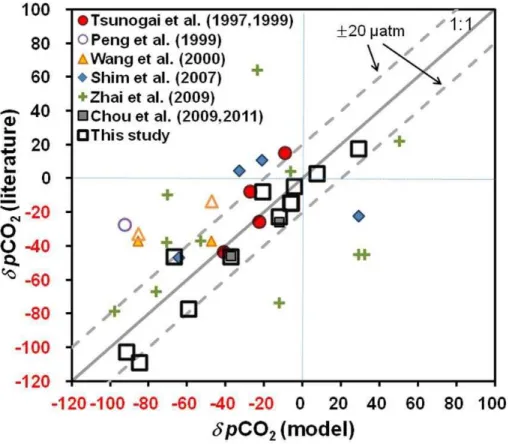
Figure 5 further shows the comparison ofδpCO2 in the same month of certain year

between the data retrieved from published references and this study and those gen-erated by model. For a comparison on an equal basis, the reported fluxes had been

10

re-calculated using the consistent source of monthly wind speed data from PenGaYi station in the ECS and the Wanninkhof’s gas transfer algorithm (1992, short-term for-mula). In addition, the Changjiang discharges in reported references were plotted in the discharge range of climatological monthly mean with±1 standard deviation (SD, 1998–

2010) as a reference level to check anomalous events (Fig. 6a). The results show there

15

were two flood surveys obtained in July 1992 and 2010 and others mostly lied within

±1 SD range of climatological mean. As a whole, most of publishedpCO2 values are

erratic away from 1 : 1 reference line outlier levels of±20 µatm (e.g., Peng et al., 1999;

Wang et al., 2000; Shim et al., 2007; Zhai et al., 2009) while some close to model out-puts (e.g., Tsunogai et al., 1999; Wang et al., 2000 in summer; Chou et al., 2011; this

20

study). The estimates with large uncertainties are mainly due to inadequate represen-tativeness of the spatial variability and limited sampling resolution. These problems in each report are briefly summarized in the remarks in Table 2 and the following text.

Tsunogai and coworkers (1997, 1999), for instance, reported the air–sea exchange fluxes of CO2 in whole ECS were only extrapolated from a single transect data of the

25

(14)

BGD

10, 13977–14007, 2013

C.-M. Tseng et al.

Title Page

Tables Figures

◭ ◮

Back Close

Full Screen / Esc

Discussion

P

a

per

|

Dis

cussion

P

a

per

|

Discussion

P

a

per

|

Discussio

n

P

a

per

|

not suitable for the use of the near-shore waters. Likewise, Peng et al’s pCO₂ data (1999) were all generated from the TA and TCO2 which were only collected in spring

and limited in low-resolution samplings. Moreover, the study area of Peng et al. (1999) was mostly located in the Kuroshio, Mixed Shelf and Taiwan Warm Current waters and lacked coverage of coastal plume waters. Higher results in spring than those by model

5

were therefore found (Fig. 6b and c), since coastal plume processes which drew the CO₂low via phytoplankton bloom near Changjiang river mouth were not observed.

Wang et al. (2000) had only two field observations in spring and summer, while their fall and winter data were computed from the Tsunogai’s empirical algorithm. Their observations lacked data from the coastal waters, although they had a wide-area

sur-10

vey (Fig. 1a). Hence, the spring pCO₂ data in the whole ECS, being derived from temperature–dependent relationship, were higher than those by model, which could not reflect the biological uptake by plankton bloom in the Changjiang plume (Fig. 6b and c). The summer results derived from salinity relationship were lower than the modeled ones. That was because of lack of the data from additional replenishment of CO2from

15

sub-surface waters by coastal upwelling. Additionally, the fall and winter data derived from Tsunogai’s algorithm could not reflect the additional CO₂by vertical mixing during the cold seasons. Therefore, those data generated from the Tsunogai’s algorithm were lower than our data by model and field observation (Fig. 6b and c).

The study in Zhai et al. (2009) was focused the areas near the Changjiang estuary

20

so that thepCO2data had large fluctuations due to complexities of coastal processes

with plume dynamics (Fig. 5). Low summer data were, for example, observed due to a strong bio-uptake of CO₂relative to ones for the whole ECS while high pCO₂in fall was due to a strong vertical mixing (Fig. 6b and c). The data of Shim et al. (2007) which were collected in the northeastern ECS showed lower in summer and higher in spring,

25

(15)

BGD

10, 13977–14007, 2013

C.-M. Tseng et al.

Title Page

Tables Figures

◭ ◮

Back Close

Full Screen / Esc

Discussion

P

a

per

|

Dis

cussion

P

a

per

|

Discussion

P

a

per

|

Discussio

n

P

a

per

|

The comparison results further indicate small-scale spatial surveys which performed in the Changjiang estuary and northern ECS area could not be representative for the whole ECS shelf.

Chou and colleagues (2009, 2011) covered the more extensive areas like our study area so that the areal mean fluxes were rather consistent with ours. After all, the

out-5

puts from our algorithm were validated by our field observations of in-situ underway

pCO2 with high spatial and temporal resolutions since 2003 (Fig. 4b–d). The model

pCO_2w results agreed well with the observed pCO_2w (R2=0.90,n=13; Fig. 4b). In addition, our algorithm can reflect the results caused by anomalous flood events, e.g., the floods of July in 1998 and 2010 causing exceptionally lowpCO2wvalues and high

10

CO₂uptakes (Table 1, Fig. 6a–c). Therefore, this assessment of annual CO₂uptake is more credible than all previous estimates (1–3 mol C m−2

yr−1

) since our better spatial and temporal coverage reduces uncertainties.

3.6 Comparison with flux estimates by di_fferent gas-exchange algorithms

Factors that affect air–sea CO2flux estimates using the two-layer gas exchange model

15

are mainly from two parts: (1) environmental forcing factors that control the gas transfer velocity,k (m s−1), and (2) thermodynamic driving potentials that affect air–seapCO2

concentration differences (Wanninkhof et al., 2009). Among these, the parameteriza-tions fork as a function of wind speed are largely empirical with inherent sources of uncertainty and therefore have a critical effect on the reliability of the flux estimates.

20

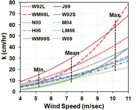
Different relationships of gas exchange with wind were empirically developed by the di_fferent approaches to calculate the gas-transfer velocity over the past decades (e.g., Liss and Merlivat, 1986 (hereafter LM86); Wanninkhof, 1992 (W92: W92S, short-term; W92L, long-term); Wanninkhof and McGillis, 1999 (WM99: WM99S; WM99L); Jacobs et al., 1999 (J99); Nightingale et al., 2000 (N00); McGillis et al., 2004 (M04); Ho et al.,

25

2006 (H06); Wanninkhof et al., 2009 (W09)). The plot of different algorithms for k

(16)

al-BGD

10, 13977–14007, 2013

C.-M. Tseng et al.

Title Page

Tables Figures

◭ ◮

Back Close

Full Screen / Esc

Discussion

P

a

per

|

Dis

cussion

P

a

per

|

Discussion

P

a

per

|

Discussio

n

P

a

per

|

gorithms significantly increase with wind speed increasing i.e., at low wind speeds are much less than those at high wind speeds (>10 m s−1

). In this study, the monthly av-erage wind speed obtained from PenGaYi station in the ECS ranged between 5 and 11 m s−1 with stronger winds in cold seasons during the northeast monsoon (Fig. 7). Varying up to almost three folds of di_fferences among di_fferent algorithms for the

cal-5

culation, the wind-inducedk was calculated to be the highest by J99 and lowest by LM86. It further demonstrates the largest source of uncertainties involved in estimat-ing air–sea CO₂ flux resides with these algorithms. Particularly, the di_fferences would increase drastically among the models developed by J99, W92L and WM99L when the wind speed increases, while the algorithm developed by N00, M04 and H06 would not

10

substantially di_ffer, as compared to W92S (Fig. 7).

In Table 3, the summary of the averaged seasonal and annual CO2fluxes between

1998 and 2010 is shown for comparison, calculated from the abovementioned 10 al-gorithms by using monthly wind speed data measured at PenGaYi station. Overall, the averaged annual CO2 fluxes range between −1.4±0.3 and −3.6±0.9 mol C m−

2

yr−1

15

with an average of−1.9±0.5 (excluding the highest value by J99). The flux results can

be basically divided into three groups: (i) high values (Avg:−3.0±0.6 mol C m−2yr−1)

by J99, W92L, and WM99L; (ii) mid-range values (−1.8±0.2) by W92S, N00, M04 and

H06; and (iii) low values (−1.4±0.1) by LM86, WM99S and W09 (Fig. 8, Table 3). The

results by W92L and WM99L are higher ca. 100 % than those by low values obtained

20

from LM86, WM99S and W09. Among moderate values, differences in flux, compared to W92S, was not much for the algorithms developed by N00, M04 and H06 (20 % lower). The W92S was further chosen for comparison since it was widely used among the reported algorithms.

The seasonal CO2 air–sea exchange fluxes estimated by the reported algorithms

25

are summarized in Table 3, which highlights the differences in seasonal variability in the CO2 sink in the ECS shelf among them. Annual CO2 fluxes from seasonal field

(17)

BGD

10, 13977–14007, 2013

C.-M. Tseng et al.

Title Page

Tables Figures

◭ ◮

Back Close

Full Screen / Esc

Discussion

P

a

per

|

Dis

cussion

P

a

per

|

Discussion

P

a

per

|

Discussio

n

P

a

per

|

annual flux was calculated to be −1.9 (±1.4, seasonal variability) mol C m−2yr−1 with

the seasonal flux ca.−3.3,−0.8±1.3 (n=3),−0.6, and−3.0 mol C m−2yr−1for spring,

summer, fall, and winter, which were almost the same as those estimated by model as shown in Table 3.

4 Conclusions

5

In this study, we have established an empirical relationship for predicting surface wa-ter pCO2 in a river-dominated marginal ECS. The empirical algorithm for calculating

pCO_2w as a function of SST and CRD successfully simulated the annual cycles of

pCO_2w,δpCO₂and the CO₂flux, which are in excellent agreement with observations. The relation was further applied to the ECS shelf areas (25–33.5◦N and 122–129◦E)

10

by using remotely sensed data of SST and the estimated area of CRD. Overall, the an-nually averaged CO₂uptake in 1998–2011 by the ECS shelf was constrained to about 1.9 mol C m−2yr−1, based on observational data and model results, which were more representative than those reported previously. This assessment of annual CO2 uptake

surpasses all previous estimates in terms of temporal and spatial coverage, and,

there-15

fore, is more reliable. Thus, the ECS was annually a net sink of atmospheric CO2with

a distinct seasonal pattern associated with inter-annual variations. The flux seasonality shows a strong sink in spring (ie., March–May) and a weak source in late summer-early fall. The weak sink status during warm periods in summer–fall is fairly sensitive to changes ofpCO2and may be easily to shift from a sink to a source altered by shrinkage

20

(18)

BGD

10, 13977–14007, 2013

C.-M. Tseng et al.

Title Page

Tables Figures

◭ ◮

Back Close

Full Screen / Esc

Discussion

P

a

per

|

Dis

cussion

P

a

per

|

Discussion

P

a

per

|

Discussio

n

P

a

per

|

Supplementary material related to this article is available online at: http://www.biogeosciences-discuss.net/10/13977/2013/

bgd-10-13977-2013-supplement.pdf.

Acknowledgements. We thank captains and crews of R/V OR-I for their assistance during LORECS cruises and G.C. Gong, project PI, for cruise logistic and hydrographic data supports.

5

Y.-F. Yeung, Y.-L. Chen, C.-S. Ji and Z.-Y. Luo assisted in lab work. This work was supported by the National Science Council (NSC, Taiwan) through grants, NSC 100 (101)-2611-M-002-004 (-015) and from the College of Science, National Taiwan University under the “Drunken Moon Lake Scientific Integrated Scientific Research Platform” grant, NTU#102R3252.

References

10

Cai, W. J., Dai, M. H., and Wang, Y. C.: Air-sea exchange of carbon dioxide in ocean margins: a province-based synthesis, Geophys. Res. Lett., 33, L12603, doi:10.1029/2006GL026219, 2006.

Chen, C. T. A. and Borges, A. V.: Reconciling opposing views on carbon cycling in the coastal ocean: continental shelves as sinks and near-shore ecosystems as sources of atmospheric

15

CO₂, Deep-Sea Res. Pt. II, 56, 578–590, 2009.

Chou, W. C., Gong, G. C., Sheu, D. D., Hung, C. C., and Tseng, T. F.: Surface distributions of carbon chemistry parameters in the East China Sea in summer 2007, J. Geophys. Res., 114, C07026, doi:10.1029/2008JC005128, 2009.

Chou, W. C., Gong, G. C., Tseng, C. M., Sheu, D. D., Hung, C. C., Chang, L. P., and Wang, L. W.:

20

The carbonate system in the East China Sea in winter, Mar. Chem., 123, 44–55, 2011.

Gong, G. C., Lee Chen, Y. L., and Liu, K. K.: Chemical hydrography and chlorophylla

distribu-tion in the East China Sea in summer: implicadistribu-tions in nutrient dynamics, Cont. Shelf Res., 16, 1561–1590, 1996.

Ho, D. T., Law, C. S., Smith, M. J., Schlosser, P., Harvey, M., and Hill, P.: Measurements of

25

(19)

BGD

10, 13977–14007, 2013

C.-M. Tseng et al.

Title Page

Tables Figures

◭ ◮

Back Close

Full Screen / Esc

Discussion

P

a

per

|

Dis

cussion

P

a

per

|

Discussion

P

a

per

|

Discussio

n

P

a

per

|

Jacobs, C. M. J., Kohsiek, W., and Oost, W. A.: Air–sea fluxes and transfer velocity of CO₂over

the North Sea: results from ASGAMAGE, Tellus B, 51(3), 629–641, 1999.

Laruelle, G. G., D ¨urr, H. H., Slomp, C. P., and Borges, A. V.: Evaluation of sinks and sources of

CO₂in the global coastal ocean using a spatially-explicit typology of estuaries and

continen-tal shelves, Geophys. Res. Lett., 37, L15607, doi:10.1029/2010GL043691, 2010.

5

Liu, K. K., Peng, T. H., and Shaw, P. T.: Circulation and biological processes in the East China Sea and the vicinity of Taiwan: an overview and a brief synthesis, Deep-Sea Res. Pt. II, 50, 1055–1064, 2003.

Liu, K.-K., Gong, G.-C., Wu, C.-R., and Lee, H.-J.: 3.2. The Kuroshio and the East China Sea, in: Carbon and Nutrient Fluxes in Continental Margins: a Global Synthesis, edited by: Liu,

K.-10

K., Atkinson, L., Qui ˜nones, R., and Talaue-McManus, L., IGBP Book Series, Springer, Berlin, 124–146, 2010.

Liss, P. S. and Merlivat, L.: Air-sea gas exchange rates: Introduction and synthesis, The Role of Air-Sea Exchange in Geochemical Cycling, 113–127, 1986.

McGillis, W. R., Edson, J. B., Zappa, C. J., Ware, J. D., McKenna, S. P., Terray, E. A., Hare,

15

J. E., Fairall, C. W., Drennan, W., Donelan, M., DeGrandpre, M. D., Wanninkhof, R., and

Feely, R. A.: Air-sea CO₂exchange in the equatorial Pacific, J. Geophys. Res. 109, C08S02,

doi:10.1029/2003JC002256, 2004.

Nightingale, P. D., Malin, G., Law, C. S., Watson, A. J., Liss, P. S., Liddicoat, M. I., Boutin, J., and Upstill-Goddard, R. C.: In situ evaluation of air–sea gas exchange parameterizations using

20

novel conservative and volatile tracers, Global Biogeochem. Cy., 14, 373–387, 2000. Peng, T. H., Hung, J. J., Wanninkhof, R., and Millero, F. J.: Carbon budget in the East China

Sea in spring, Tellus B, 51, 531–540, 1999.

Shim, J., Kim, D., Kang, Y. C., Lee, J. H., Jang, S.-T., and Kim, C.-H.: Seasonal variations in

pCO₂and its controlling factors in surface seawater of the northern East China Sea, Cont.

25

Shelf Res., 27, 2623–2636, 2007.

Takahashi, T., Olafsson, J., Goddard, J. G., Chipman, D. W., and Sutherland, S.: Seasonal

vari-ation of CO₂and nutrients in the high-latitude surface oceans: a comparative study, Global

Biogeochem. Cy., 7, 843–878, 1993.

Tseng, C. M., Wong, G. T. F., Lin, I. I., Wu, C. L., and Liu, K. K.: A unique pattern in

phyto-30

(20)

BGD

10, 13977–14007, 2013

C.-M. Tseng et al.

Title Page

Tables Figures

◭ ◮

Back Close

Full Screen / Esc

Discussion

P

a

per

|

Dis

cussion

P

a

per

|

Discussion

P

a

per

|

Discussio

n

P

a

per

|

Tseng, C. M., Wong, G. T. F., Chou, W. C., Lee, B. S., Sheu, D. D., and Liu, K. K.: Temporal Variations in the carbonate system in the upper layer at the SEATS station, Deep-Sea Res. Pt. II, 54, 1448–1468, 2007.

Tseng, C. M., Liu, K. K., Wang, L. W., and Gong, G. C.: Anomalous hydrographic and biological conditions in the northern South China Sea during the 1997–1998 El Ni ˜no

5

and comparisons with the equatorial Pacific, Deep-Sea Res. Pt. I, 56, 2129–2143, doi:10.1016/j.dsr.2009.09.004, 2009a.

Tseng, C. M., Gong, G. C., Wang, L. W., Liu, K. K., and Yang, Y.: Anomalous biogeochemical conditions in the northern South China Sea during the El-Ni ˜no events between 1997 and 2003, Geophys. Res. Lett., 36, L14611,doi:10.1029/2009GL038252, 2009b.

10

Tseng, C. M., Liu, K. K., Gong, G. C., Shen, P. Y., and Cai, W. J.: CO₂ uptake in the East

China Sea relying on Changjiang runoff is prone to change, Geophys. Res. Lett., 38,

doi:10.1029/2011GL049774, L24609, 2011.

Tsunogai, S., Watanabe, S., Nakamura, J., Ono, T., and Sato, T.: A preliminary study of carbon system in the East China Sea, J. Oceanogr., 53, 9–17, 1997.

15

Tsunogai, S., Watanabe, S., and Sato, T.: Is there a continental shelf pump for the absorption

of atmospheric CO₂?, Tellus B, 51, 701–712, 1999.

Wang, S. L., Chen, C. T. A., Hong, G. H., and Chung, C. S.: Carbon dioxide and related param-eters in the East China Sea, Cont. Shelf Res., 20, 525–544, 2000.

Wanninkhof, R.: Relationship between wind speed and gas exchange over the ocean, J.

Geo-20

phys. Res., 97, 7373–7382, 1992.

Wanninkhof, R. and McGillis, W. R.: A cubic relationship between air–sea CO₂exchange and

wind speed, Geophys. Res. Lett., 26, 1889–1892, 1999.

Wanninkhof, R., Asher, W. E., Ho, D. T., Sweeney, C., and McGillis, W. R.: Advances in quan-tifying air–sea gas exchange and environmental forcing, Annu. Rev. Mar. Sci., 1, 213–244,

25

doi:10.1146/annurev.marine.010908.163742, 2009.

Walsh, J. J.: Importance of continental margins in the marine biological cycling of carbon and nitrogen, Nature, 350, 53–55, 1991.

Weiss, R. F.: Carbon dioxide in water and seawater: the solubility of a non-ideal gas, Mar. Chem., 2, 203– 215, 1974.

30

Zhai, W. and Dai, M.: On the seasonal variation of air–sea CO₂fluxes in the outer Changjiang

(21)

BGD

10, 13977–14007, 2013

C.-M. Tseng et al.

Title Page

Tables Figures

◭ ◮

Back Close

Full Screen / Esc

Discussion

P

a

per

|

Dis

cussion

P

a

per

|

Discussion

P

a

per

|

Discussio

n

P

a

per

|

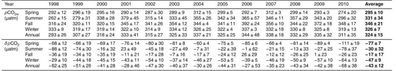
Table 1.The seasonal and annual average CO₂ results between 1998 and 2010 in the ECS shelf.

Year 1998 1999 2000 2001 2002 2003 2004 2005 2006 2007 2008 2009 2010 Average

pCO2w Spring 292±12 296±19 295±16 290±14 287±30 289±9 312±15 299±5 292±7 312±3 299±14 293±3 274±20 295±10

(µatm) Summer 262±15 279±31 338±28 379±45 315±14 333±45 355±26 342±34 365±57 346±11 357±29 343±20 296±32 331±34

Fall 316±24 320±11 320±15 345±17 341±26 354±12 344±4 341±11 392±24 356±10 344±22 372±18 348±17 346±21

Winter 333±9 319±17 319±14 322±10 314±9 334±12 326±25 322±4 337±3 332±18 330±8 325±8 319±13 326±7

Annual 293±26 307±27 318±24 333±41 315±27 325±33 337±21 325±25 344±48 338±18 332±29 335±32 311±35 324±15 δpCO2 Spring −68±12 −66±19 −69±17 −76±14 −80±30 −81±8 −60±4 −75±5 −85±6 −66±4 −81±14 −89±4 −111±19 −77±7

(µatm) Summer −88±12 −74±30 −16±32 23±49 −45±18 −27±49 −7±31 −22±39 −1±62 −21±15 −13±33 −27±25 −78±37 −30±32

Fall −36±19 −34±10 −35±19 −11±21 −17±28 −7±16 −17±7 −24±12 26±29 −12±12 −26±25 1±23 −26±23 −17±17

Winter −29±10 −44±18 −45±15 −43±11 −54±10 −37±14 −46±27 −53±5 −39±5 −46±19 −50±9 −57±10 −64±13 −47±9

(22)

BGD

10, 13977–14007, 2013

C.-M. Tseng et al.

Title Page Abstract Introduction Conclusions References Tables Figures ◭ ◮ ◭ ◮ Back Close

Full Screen / Esc

Printer-friendly Version Interactive Discussion Discussion P a per | Dis cussion P a per | Discussion P a per | Discussio n P a per |

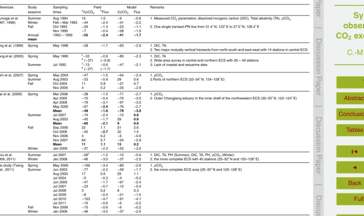
Table 2.Summary of the CO₂results in the ECS reported in the previous studies and obtained from this study.

References Study Sampling Field Model Remarks seasons times a_δp_CO

2

b_Flux _δp_CO

2 Flux

Tsunogai et al. (1997, 1999)

Summer Winter

Aug 1994 Feb∼Mar 1993

15 −44 1.0 −2.4 −9 −41 −0.6 −2.2

1. Measured CO2parameters: dissolved inorganic carbon (DIC), Total alkalinity (TA),pCO2.

Fall Oct 1993 Nov 1995 −26 −7 −1.3 −0.4 −23 −28 −1.1 −1.5

2. One single transect-PN line from 31.4◦_{N, 123}◦_{E to 27.5}◦_{N, 128.4}◦_E

Annual

mean

1993∼1995 −55 −2.4 −41 −1.7

Peng et al. (1999) Spring May 1996 −28 −1.7 −93 −2.9 1. DIC, TA;

2. Two major mutually vertical transects from north-south and east-west with 14 stations in central ECS Wang et al. (2000) Spring May 1995 c

−33

d₍

−37) −0.9 (−0.9)

−85 −2.3 1. DIC, TA

2. Wide-area survey in central and northern ECS with 26∼49 stations Summer Jul 1992 c

−13

e₍

−37) −0.6 (−1.7)

−47 −2.1 3. Lack of coastal and estuarine data Shim et al. (2007) Spring

Summer Fall May 2004 Aug 2003 Oct 2004 Nov 2005 −47 −23 11 4 −1.5 −0.9 0.8 0.2 −64 29 −21 −33 −2.4 0.6 0.7 −2.9

1.pCO2

2.Parts of northern ECS (32–34◦_{N, 124–128}◦_E)

Zhai et al. (2009) Spring Mar 2008 Apr 2005 Apr 2008 May 2005 Mean −38 −10 −79 −67 −48 −1.5 −0.4 −3.1 −2.4 −1.8 −71 −70 −97 −76 −79 −2.7 −3.0 −3.5 −2.7 −3.0

1.pCO2

2. Outer Changjiang estuary in the inner shelf of the northwestern ECS (30–33◦_{N, 122–124}◦_E)

Summer Jul 2007 Aug 2003 Mean −74 −45 −60 −2.4 −1.7 −2.1 −12 29 9 0.6 0.6 0.0

Fall Sep 2006 Oct 2006 Nov 2006 Nov 2007 Mean 22 −45 4 64 11 1.1 −2.7 0.2 5.7 1.1 51 32 −6 −24 13 2.6 1.4 −0.6 −2.9 0.2

Winter Jan 2006 −37 −2.3 −53 −3.0 Chou et al.

(2009, 2011)

Summer Winter

Jul 2007 Jan 2008

−26c

−46 −1.2 −3.0 −12 −37 −0.6 −2.5

1. DIC, TA, PH (Summer), DIC, TA, PH,pCO2(Winter)

2. the more complete ECS with 40 stations (25–32◦_{N and 120–128}◦_E)

This study (Tseng et al., 2011)

Spring Summer May 2009 Jun 2003 Aug 2003 Jul 2004 Jun 2005 Jul 2007 Jul 2008 Jul 2009 Jul 2010 Jul 2011 −109 −77 17 −5 −47 −23 3 −8 −103 −15 −3.4 −2.2 0.6 −0.3 −1.7 −0.7 0.2 −0.4 −4.7 −0.6 −85 −59 29 −4 −67 −12 8 −21 −91 −6 −2.6 −1.7 1.1 −0.2 −2.4 −0.4 0.3 −1.0 −4.1 −0.2

1.pCO2

2. the more complete ECS area (25–32◦_{N and 120–128}◦_E)

Fall Winter Nov 2006 Jan 2008 −15 −46 −0.6 −3.0 −6 −37 −0.2 −2.5 a

Units inδpCO2and CO2flux are µatm and mol C m− 2

yr−1

, respectively.

b

Re-calculated by wind speed data at PenGaYi and Wnninkkhof’s gas transfer algorithm (1992, short-term formula).

c

Average of all stations.

d_{Averaged by values derived from}_p_CO

2-salinity relationship. e_{Averaged by values derived from}_p_CO

(23)

BGD

10, 13977–14007, 2013

C.-M. Tseng et al.

Title Page

Tables Figures

◭ ◮

Back Close

Full Screen / Esc

Discussion

P

a

per

|

Dis

cussion

P

a

per

|

Discussion

P

a

per

|

Discussio

n

P

a

per

|

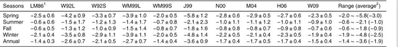
Table 3.Seasonal average CO₂fluxes between 1998 and 2010 derived from the reported gas-transfer algorithms.

Seasons LM861 W92L W92S WM99L WM99S J99 N00 M04 H06 W09 Range (average2)

Spring −2.5±0.6 −4.2±0.9 −3.3±0.7 −3.9±1.0 −2.0±0.5 −5.8±1.2 −2.8±0.6 −2.9±0.5 −2.7±0.6 −2.3±0.5 −2.0∼ −5.8(−3.0) Summer −0.6±0.6 −1.5±1.7 −1.2±1.3 −1.4±1.7 −0.7±0.8 −2.1±2.3 −1.0±1.1 −1.1±1.2 −1.0±1.1 −0.9±1.0 −0.6∼ −2.1 (−1.0) Fall −0.6±0.5 −1.3±1.2 −1.0±0.9 −1.5±1.4 −0.8±0.7 −1.8±1.6 −0.8±0.8 −0.8±0.7 −0.9±0.8 −0.7±0.6 −0.6∼ −1.8 (−0.9) Winter −2.1±0.4 −3.5±0.8 −2.9±1.1 −3.9±1.1 −2.0±0.5 −4.8±1.4 −2.2±0.5 −2.1±0.4 −2.3±0.5 −1.9±0.4 −1.9∼ −4.8 (−2.5) Annual −1.4±0.3 −2.6±0.7 −2.1±0.5 −2.7±0.7 −1.4±0.4 −3.6±0.9 −1.7±0.4 −1.7±0.5 −1.7±0.4 −1.5±0.4 −1.4∼ −3.6 (−1.9)

1

Abbreviations denote references with gas-transfer equations: LM86: Liss and Merlivat (1986),

k600=2.85×u−9.65(3.6< u <13.0) W92S: Wanninkhof (1992, short-term),

k660=0.31×u 2

W92L: Wanninkhof (1992, long-term),

k660=0.39×u2

WM99S: Wanninkhof and McGillis (1999, short-term),

k660=1.09×u−0.333×u2 +0.078×u3

WM99L: Wanninkhof and McGillis (1999, long-term),

k660=0.0283×u3

J99: Jacobs et al. (1999),

k660=0.54×u2

N00: Nightingale et al. (2000),

k600=0.333×u+0.222×u 2

M04: McGillis et al. (2004),

k660=0.014×u3₊_8.2

H06: Ho et al. (2006),

k600=0.266×u2

W09: Wanninkhof et al.(2009),

k660=3+0.1×u−0.064×u2 +0.011×u3

.

2

(24)

BGD

10, 13977–14007, 2013

C.-M. Tseng et al.

Title Page

Tables Figures

◭ ◮

Back Close

Full Screen / Esc

Discussion

P

a

per

|

Dis

cussion

P

a

per

|

Discussion

P

a

per

|

Discussio

n

P

a

per

|

KW TSW

CDW

SMW

TWC

31

Changjiang River

East China

Sea

Pacific Ocean

pCO2(µatm) Flux(mol C m-2 y-1)

31 31

(a) (b)

(c) (d)

Region B

Region S

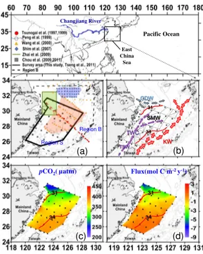
Fig. 1.Maps of the study areas in the ECS showing(a)the previously published CO₂-related studies (e.g., Tsunogai et al., 1997, 1999; Peng et al., 1999; Wang et al., 2000; Shim et al., 2007; Zhai et al., 2009; Chou et al., 2009, 2011; Tseng et al., 2011). The surveyed area of Tseng et al. (2011) and this study is Region S. The area outlined by dashed line for modeled

synthesis is Region B.(b)Hydrographic stations (black dots) and cruise track of the underway

pCO₂ measurements (dashed line) with sea surface salinity (SSS) contours and circulation

patterns in the ECS in summer. KW–Kuroshio Water; TSW–Taiwan Strait Water; TWC–Taiwan

Warm Current, SMW–Shelf Mixed Water; CDW–Changjing Diluted Water.;(c) the composite

distributions of surface waterpCO₂ (µatm); and(d)air–sea CO₂exchange flux observed

(25)

BGD

10, 13977–14007, 2013

C.-M. Tseng et al.

Title Page

Tables Figures

◭ ◮

Back Close

Full Screen / Esc

Discussion

P

a

per

|

Dis

cussion

P

a

per

|

Discussion

P

a

per

|

Discussio

n

P

a

per

|

Fig. 2. Linear regression relationships between areal mean AVHRR-SST in two model

re-gions, i.e.,(a)S and(b)B, and field observed areal mean SST in cruise survey area.

(26)

BGD

10, 13977–14007, 2013

C.-M. Tseng et al.

Title Page

Tables Figures

◭ ◮

Back Close

Full Screen / Esc

Discussion

P

a

per

|

Dis

cussion

P

a

per

|

Discussion

P

a

per

|

Discussio

n

P

a

per

|

Fig. 3.Correlation between monthly average NpCO₂ and CRD (black square) was observed

during warm cruises from May to November between 1998 and 2011: observed NpCO₂about

455.1 µatm (blue dot) and the computed NpCO₂ 397.7 µatm (dotted circle) at the CRD at

10 211 m3s−1

during the January cruise.

(27)

BGD

10, 13977–14007, 2013

C.-M. Tseng et al.

Title Page

Tables Figures

◭ ◮

Back Close

Full Screen / Esc

Discussion

P

a

per

|

Dis

cussion

P

a

per

|

Discussion

P

a

per

|

Discussio

n

P

a

per

|

32

Fig. 4.Time-series variations (model results with observed data of 12 cruises) in monthly areal

mean(a)SST and CRD,(b)pCO_2wandpCO_2a,(c)δpCO₂, and(d)CO₂flux in sea surface of

the ECS shelf (“+”: sea to air; “₋”: air to sea) between 1998 and 2011. The tick on the time axis

(28)

BGD

10, 13977–14007, 2013

C.-M. Tseng et al.

Title Page

Tables Figures

◭ ◮

Back Close

Full Screen / Esc

Discussion

P

a

per

|

Dis

cussion

P

a

per

|

Discussion

P

a

per

|

Discussio

n

P

a

per

|

Fig. 5.δpCO₂comparison between the data retrieved from published references and this study and those generated by model at the same surveying time.

(29)

BGD

10, 13977–14007, 2013

C.-M. Tseng et al.

Title Page

Tables Figures

◭ ◮

Back Close

Full Screen / Esc

Discussion

P

a

per

|

Dis

cussion

P

a

per

|

Discussion

P

a

per

|

Discussio

n

P

a

per

|

34

Fig. 6.Seasonal monthly patterns revealed in observational data of (a)CRD, (b)δpCO₂and

(c)air–sea CO₂ flux, obtained from published references and from field data in this study and

model results. The thick curves denotes the climatological mean and the dash curves denote

(30)

BGD

10, 13977–14007, 2013

C.-M. Tseng et al.

Title Page

Tables Figures

◭ ◮

Back Close

Full Screen / Esc

Discussion

P

a

per

|

Dis

cussion

P

a

per

|

Discussion

P

a

per

|

Discussio

n

P

a

per

|

Fig. 7.Comparison among different algorithms for flux calculation against wind speed (LM86 corresponds to Liss and Merlivat (1986); other labels see in Table 3). Black dashed lines in Min., Mean and Max. denote the minimum, average and maximum monthly average wind speeds obtained from PenGaYi station in the ECS during the study period.