AMTD
7, 2879–2928, 2014Ecosystem fluxes of hydrogen
L. K. Meredith et al.
Title Page
Abstract Introduction
Conclusions References
Tables Figures
◭ ◮
◭ ◮
Back Close
Full Screen / Esc
Printer-friendly Version Interactive Discussion
Discussion
P
a
per
|
D
iscussion
P
a
per
|
Discussion
P
a
per
|
Discuss
ion
P
a
per
|
Atmos. Meas. Tech. Discuss., 7, 2879–2928, 2014 www.atmos-meas-tech-discuss.net/7/2879/2014/ doi:10.5194/amtd-7-2879-2014
© Author(s) 2014. CC Attribution 3.0 License.
Atmospheric Measurement
Techniques
Open Access
Discussions
This discussion paper is/has been under review for the journal Atmospheric Measurement Techniques (AMT). Please refer to the corresponding final paper in AMT if available.
Ecosystem fluxes of hydrogen:
a comparison of flux-gradient methods
L. K. Meredith1,*, R. Commane2, J. W. Munger2, A. Dunn3, J. Tang4, S. C. Wofsy2, and R. G. Prinn1
1
Center for Global Change Science, Massachusetts Institute of Technology, Cambridge, Massachusetts, USA
2
School of Engineering and Applied Sciences and Department of Earth and Planetary Sciences, Harvard University, Cambridge, Massachusetts, USA
3
Department of Physical and Earth Science, Worcester State University, Worcester, Massachusetts, USA
4
Ecosystems Center, Marine Biological Laboratory, Woods Hole, Massachusetts, USA
*
now at: Environmental Earth System Science, Stanford University, Stanford, California, USA
Received: 10 March 2014 – Accepted: 12 March 2014 – Published: 25 March 2014
Correspondence to: L. K. Meredith ([email protected])
AMTD
7, 2879–2928, 2014Ecosystem fluxes of hydrogen
L. K. Meredith et al.
Title Page
Abstract Introduction
Conclusions References
Tables Figures
◭ ◮
◭ ◮
Back Close
Full Screen / Esc
Printer-friendly Version Interactive Discussion
Discussion
P
a
per
|
D
iscussion
P
a
per
|
Discussion
P
a
per
|
Discuss
ion
P
a
per
|
Abstract
Our understanding of biosphere-atmosphere exchange has been considerably en-hanced by eddy-covariance measurements, however there remain many trace gases,
such as molecular hydrogen (H2), for which there are no suitable analytical methods
to measure their fluxes by eddy covariance. In such cases, flux-gradient methods can
5
be used to calculate ecosystem-scale fluxes from vertical concentration gradients. The
budget of atmospheric H2 is poorly constrained by the limited available observations,
thus the ability to quantify and characterize the sources and sinks of H2by flux-gradient
methods in various ecosystems is important. We developed an approach to make
non-intrusive, automated measurements of ecosystem-scale H2fluxes both above and
be-10
low the forest canopy at the Harvard Forest in Petersham, MA for over a year. We used three flux-gradient methods to calculate the fluxes: two similarity methods that
do not rely on a micrometeorological determination of the eddy diffusivity, K, based
on (1) trace gases or (2) sensible heat and one flux-gradient method that (3)
parame-terizesK. We quantitatively assessed the flux-gradient methods on CO2 and H2O by
15
comparison to their simultaneous independent flux measurements via eddy covariance and chambers. All three flux-gradient methods performed well in certain locations,
sea-sons, and times of day, and the best methods were trace gas similarity above andK
pa-rameterization below the canopy. Sensible heat similarity required several independent measurements and the results were more variable, in part because those data were
20
only available in the winter when heat fluxes and temperature gradients were small and
difficult to measure. Biases were often observed between flux-gradient methods and
the independent flux measurements, including at least a 26 % difference in nocturnal
eddy-derived Net Ecosystem Exchange (NEE) and soil chamber measurements. All
flux-gradient methods used to calculate above and below canopy H2 fluxes pointed to
25
soil uptake as the main driver of H2exchange at Harvard Forest. H2fluxes calculated
in a summer period agreed within their uncertainty and indicated that H2 deposition
AMTD
7, 2879–2928, 2014Ecosystem fluxes of hydrogen
L. K. Meredith et al.
Title Page
Abstract Introduction
Conclusions References
Tables Figures
◭ ◮
◭ ◮
Back Close
Full Screen / Esc
Printer-friendly Version Interactive Discussion
Discussion
P
a
per
|
D
iscussion
P
a
per
|
Discussion
P
a
per
|
Discuss
ion
P
a
per
|
1 Introduction
Atmospheric H2, with a global average mole fraction of 530 ppb (parts per billion; 10−
9
;
nmol mol−1), exerts a notable influence on atmospheric chemistry and radiation (Novelli
et al., 1999). H2is scavenged by the hydroxyl radical (OH radical), thereby attenuating
the ability of OH to scavenge potent greenhouse gases, like methane (CH4) from the
5
atmosphere, which classifies H2 as an indirect greenhouse gas (Novelli et al., 1999).
H2 is also a significant source of water vapor to the stratosphere, and as such may
adversely perturb stratospheric ozone chemistry (Solomon, 1999; Tromp et al., 2003;
Warwick et al., 2004). The two major atmospheric H2sources, photochemical
produc-tion from methane and non-methane hydrocarbons and combusproduc-tion of fossil fuels and
10
biomass, are nearly balanced by its sinks so atmospheric concentrations are stable
(Novelli et al., 1999; Xiao et al., 2007). The major H2sinks are soil consumption,
repre-senting about 81±8 % of the total sink, and oxidation by OH being about 17±3 % based
on a global inversion of sparse atmospheric H2 measurements (Xiao et al., 2007).
Al-though the global atmospheric H2 budget has been derived by a variety of methods,
15
it remains poorly constrained at the regional level, disputed at the global level, and a process-based understanding is lacking (as reviewed by Ehhalt and Rohrer, 2009).
Therefore, there are large uncertainties in the estimated impact of changes to the H2
biogeochemical cycle that might arise from changes in energy use, land use, and cli-mate. Field and laboratory measurements are needed to improve the process-level
20
understanding of atmospheric H2sources and sinks, especially regarding its particular
sensitivity to biological activity in the soils.
The paucity of data on key H2processes is related to difficulties in measuring sources
and sinks in situ, in particular the soil sink. H2soil uptake is typically measured using
flux chambers (e.g., Conrad and Seiler, 1980; Lallo et al., 2008; Smith-Downey et al.,
25
AMTD
7, 2879–2928, 2014Ecosystem fluxes of hydrogen
L. K. Meredith et al.
Title Page
Abstract Introduction
Conclusions References
Tables Figures
◭ ◮
◭ ◮
Back Close
Full Screen / Esc
Printer-friendly Version Interactive Discussion
Discussion
P
a
per
|
D
iscussion
P
a
per
|
Discussion
P
a
per
|
Discuss
ion
P
a
per
|
from chamber measurements up to landscape scale is difficult, however (Baldocchi
et al., 1988). Boundary layer methods have been used to calculate H2soil uptake rates
from H2 mole fraction measurements and assumptions about atmospheric winds and
mixing, boundary layer height, and/or the uptake rates of other trace gases (Simmonds et al., 2000; Steinbacher et al., 2007). The need for assumptions in these methods
5
can introduce large uncertainties into reported H2fluxes. Most data is focused on soil
processes, and we have little information about any other processes in the canopy that affect H2.
Despite the limitations of these traditional methods, few alternatives are available for
the measurement or estimation of atmospheric H2 fluxes. The gas chromatographic
10
methods used to measure H2are slow (>4 min), which precludes use of eddy
covari-ance techniques that rely on high-frequency measurement of the covariation of the trace gas mole fraction with the vertical wind component. In such cases, where no
high-accuracy fast-response instrument (≥1 Hz sampling frequency) is available, a
va-riety of micrometeorological methods under the umbrella of flux-gradient theory can be
15
used to non-intrusively measure the biosphere-atmosphere exchange of trace gases
from relatively slow (<<1 Hz) measurements of vertical gradients of trace gas mole
fractions (Fuentes et al., 1996; Meyers et al., 1996). Flux-gradient methods assume that fluxes are equal to the (negative) gradient of the quantity in question scaled by the rate of turbulent exchange. These methods can be automated for near
continu-20
ous data collection, and by averaging over time, the spatial heterogeneity within the tower footprint is integrated (Baldocchi et al., 1988). As a result, flux-gradient methods avoid some of the aforementioned problems that arise from the use of flux chambers and box models. These methods are also useful in cases where fluxes are small and fast-response instruments lack the precision to resolve deviations in trace gas mole
25
fraction from background levels (Simpson et al., 1998). The structure of the
turbu-lence below the canopy can make eddy covariance measurements difficult, and
AMTD
7, 2879–2928, 2014Ecosystem fluxes of hydrogen
L. K. Meredith et al.
Title Page
Abstract Introduction
Conclusions References
Tables Figures
◭ ◮
◭ ◮
Back Close
Full Screen / Esc
Printer-friendly Version Interactive Discussion
Discussion
P
a
per
|
D
iscussion
P
a
per
|
Discussion
P
a
per
|
Discuss
ion
P
a
per
|
a three-dimensional process, the existence of steady-state conditions, horizontal ho-mogeneity in the source-sink distributions, and flat topography (Baldocchi et al., 1988).
Recognizing the potential for flux-gradient methods for determining the H2 flux, we
designed, constructed, and evaluated a fully automated, continuous measurement
sys-tem for determining H2 fluxes in a forest ecosystem by three different flux-gradient
5
methods: (1) trace-gas similarity, (2) sensible heat similarity, and (3)K
parameteriza-tion. Critical issues in instrument design and performance for making flux-gradient mea-surements were considered, including precision, sampling error, and bias. The validity
of each flux-gradient method was demonstrated by application to CO2and H2O fluxes,
for which simultaneous eddy covariance or chamber flux measurements were available
10
for comparison. Finally, H2fluxes were calculated using the flux-gradient methods in the
above- and below-canopy environment. The approach and findings could be extended
to other trace gases that present similar measurement challenges to H2.
2 Experimental
2.1 Measurement site
15
The study site, Harvard Forest (42◦32′N, 72◦11′W; elevation 340 m), is located in
Pe-tersham, Massachusetts, approximately 100 km west of Boston, Massachusetts. The largely deciduous 80 to 110-year old forest is dominated by red oak, red maple, red and white pine, and hemlock (Urbanksi et al., 2007). Harvard Forest soils are acidic and originate from sandy loam glacial till (Allen, 1995). Measurements presented in
20
this study were made from November 2010 to March 2012 at the Environmental Mea-surement Station (EMS) (Wofsy et al., 1993), located in the Prospect Hill tract of Harvard Forest. The station is surrounded for several kilometers by moderately hilly terrain and relatively undisturbed forest since the 1930s. Previous work at the site found no evidence for anomalous flow patterns that would interfere with eddy-flux
25
AMTD
7, 2879–2928, 2014Ecosystem fluxes of hydrogen
L. K. Meredith et al.
Title Page
Abstract Introduction
Conclusions References
Tables Figures
◭ ◮
◭ ◮
Back Close
Full Screen / Esc
Printer-friendly Version Interactive Discussion
Discussion
P
a
per
|
D
iscussion
P
a
per
|
Discussion
P
a
per
|
Discuss
ion
P
a
per
|
within 20 % (Goulden et al., 1996), and about 80 % of the turbulent fluxes originate within a 0.7–1 km radius of the tower (Sakai et al., 2001; Urbanski et al., 2007).
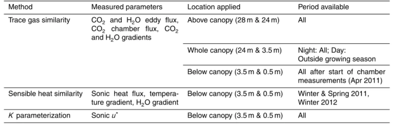
2.2 Instrumentation
An instrument system was designed to measure mole fraction gradients and ancillary
variables needed to calculate H2 fluxes above and below the forest canopy at four
5
heights (Fig. 1). H2 mole fractions were measured with a gas chromatograph (GC,
model 6890, Agilent Technologies) equipped with a pulsed discharge helium ioniza-tion detector (HePDD, model D-3 PDD, Valco Instruments Co. Inc. (VICI)) and two
columns (HayeSep DB, 1/8 in OD stainless steel, 2 m pre-column 80/100 and 4.5 m
analytical column 100/120, Chromatographic Specialties). A 2-position, 12-port
injec-10
tion valve (UW type, 1/16 in ports, M-type rotor, purged housing, VICI) was used to
introduce 2 mL samples and control the chromatographic timing. The GC-HePDD was run with research grade helium carrier gas (99.9999 % purity, Airgas) and was config-ured as in Novelli et al. (2009), with the exception of a shorter pre-column to reduce the analysis time to 4 min (Meredith, 2012: Figs. 2–3). Sample loop pressure
(trans-15
ducer model 722B13TFF3FA, MKS Instruments) and temperature (thermistor affixed
to sample loop) were measured to quantify the exact mass of sample air injected. The GC sample stream was dried using a Nafion drying tube (MD-070-12S-2, Perma
Pure). CO2 and H2O mole fractions were measured at four heights using a pair of
non-dispersive, infrared gas analyzers (Model 6262, LI-COR) configured to measure
20
vertical gradients (Dunn et al., 2009).
Gas sampling inlets were installed at 24 m and 28 m on the EMS tower above the forest canopy and at 0.5 m and 3.5 m on a below-canopy tower erected 14 m to the north-northwest of the EMS tower in an area of undisturbed vegetation and soil (Fig. 2). The leaf foliage distribution (Fig. 2.) during summer at the Harvard Forest EMS site is
25
top-heavy (median height of 18 m), and is important to consider for its interactions with the turbulent structures at the site (Parker, unpublished data). Tubing lines (OD 1/4
AMTD
7, 2879–2928, 2014Ecosystem fluxes of hydrogen
L. K. Meredith et al.
Title Page
Abstract Introduction
Conclusions References
Tables Figures
◭ ◮
◭ ◮
Back Close
Full Screen / Esc
Printer-friendly Version Interactive Discussion
Discussion
P
a
per
|
D
iscussion
P
a
per
|
Discussion
P
a
per
|
Discuss
ion
P
a
per
|
PFA, Cole Palmer) containing 2 µm pore size filters (Zefluor™, Pall Corporation) and
inverted teflon funnels to protect the tubing inlet from precipitation. During the normal
sampling routine, H2GC-HePDD measurements were made throughout the canopy at
28 m, 24 m, 3.5 m, and 0.5 m over a 16 min cycle. Meanwhile, continuous gas streams from each inlet were drawn through the IRGA rack and 1 min measurement cycles of
5
CO2 and H2O were made from either the 28 m and 0.5 m or 24 m and 3.5 m inlets at
a given time. Each sample stream was mixed in 2 L glass integrating volumes mixed by computer fans (Meredith, 2012; Fig. A1). Three times per week, a nulling procedure was performed to test for bias between sampling inlets by sampling from a common gas inlet installed 2 m above the ground that passed through an unmixed 25 L nulling
10
reservoir (glass carboy).
Custom-designed small footprint aspirated temperature shields (Dunn et al., 2009) containing thermistors (YSI) were co-located with the gas inlets. Temperature data
were corrected for offsets between the sensors, which were determined on two
oc-casions by temporarily co-locating temperature shields. 3-D sonic anemometers were
15
installed on the small tower at 2 m (CSAT3, Campbell Scientific) and on the EMS tower at 29 m (Applied Technologies). 3-D winds were rotated to the plane where the mean vertical wind is zero (Wilczak et al., 2001). Data acquisition/logging and sample valve control was handled by Campbell Scientific CR10X data loggers. GCwerks (Version 3.02-2, Peter Salameh, Scripps Institute of Oceanography, http://gcwerks.com) was
20
used for gas chromatograph control and peak integration (example chromatogram in Meredith, 2012; Figs. 2–4).
Independent eddy covariance CO2 and H2O flux measurements were made above
the forest canopy (Urbanski et al., 2007). The soil-atmosphere flux of CO2 was
mea-sured using an automated flux chamber system located approximately 0.6 km south of
25
AMTD
7, 2879–2928, 2014Ecosystem fluxes of hydrogen
L. K. Meredith et al.
Title Page
Abstract Introduction
Conclusions References
Tables Figures
◭ ◮
◭ ◮
Back Close
Full Screen / Esc
Printer-friendly Version Interactive Discussion
Discussion
P
a
per
|
D
iscussion
P
a
per
|
Discussion
P
a
per
|
Discuss
ion
P
a
per
|
control chambers not placed on a root-exclusion plot are used here. During the mea-surement cycle, the air inside the chamber was pumped through the flow meter and the IRGA, and back to the chamber. The chamber was vented to equalize pressure be-tween the inside and outside of the chamber. The chamber top was closed for 2–3 min
during the measurement period. CO2 concentration was read by the IRGA every 12 s
5
and recorded in the data logger. The CO2 flux was calculated based on the increase
in CO2concentration inside the chamber during the measurement period of time. The
flux measurements were rotated among the chambers within a half-hour period. Thus a data frequency of half-hour interval was obtained for each chamber.
2.3 Calibration
10
Trace-gas measurements were calibrated every 1.5 and 3 h for H2 and CO2,
respec-tively. GC-HePDD calibrations were based on duplicate sampling from an H2calibration
standard of compressed air from Niwot Ridge in an electropolished stainless steel tank (34 L, Essex Industries) referenced against the NOAA Earth System Research Lab-oratory Global Monitoring Division (ESRL/GMD) primary standards on their in-house
15
instrument before 501.5 (±10) ppb and after 499.0 (±7.5) ppb the experiment. H2levels
were stable in our calibration cylinder, as has been reported for other steel cylinders, but not for many aluminum tanks (Jordan and Steinberg, 2011). The GC-HePDD re-sponse was stable over the study period (Meredith, 2012; Figs. 2–9 and 2–10).
CO2 calibrations were performed using three CO2 span gases (HI∼500 ppm, MID
20
∼420 ppm, and LO∼350 ppm) traceable to the NOAA and World Meteorological
Or-ganization (WMO) CO2 scales. IRGA zeros were determined by periodically passing
ambient air through a CO2 scrubber (soda lime) and desiccant (magnesium
perchlo-rate) trap. Water vapor measurements were calibrated on one occasion with a dew point generator (Model 610, LI-COR). Simultaneous, co-located mole fraction
measure-25
ments of CO2 and H2O (instrument from this study vs. the independent EMS system)
were used to derive scaling factors for comparison to the EMS eddy covariance fluxes
AMTD
7, 2879–2928, 2014Ecosystem fluxes of hydrogen
L. K. Meredith et al.
Title Page
Abstract Introduction
Conclusions References
Tables Figures
◭ ◮
◭ ◮
Back Close
Full Screen / Esc
Printer-friendly Version Interactive Discussion
Discussion
P
a
per
|
D
iscussion
P
a
per
|
Discussion
P
a
per
|
Discuss
ion
P
a
per
|
R2=0.84) and H2O (slope=1.085,R
2
=0.98). A detailed description of the instrument
design, parts, and calibration is available online (Meredith, 2012).
2.4 Gradient measurement considerations
2.4.1 Precision
Application of the three flux-gradient methods relies on the ability to resolve vertical
5
gradients in mole fraction or temperature. The problem is not trivial as vigorous turbu-lent mixing can cause the gradients, even those originating from strong source or sink
processes, to be quite small. In this study, we aimed to resolve H2gradients both above
and below the forest canopy. Reported gradients between inlets at 3.5 and 0.5 m over
a grassland in Quebec (Constant et al., 2008), which were typically a<5 % difference
10
over the 3 m, but somewhat larger at night under stable nocturnal conditions, provided a starting point for specifying the instrument precision that would be required for the Harvard Forest measurements. Although there were no previous above-canopy
mea-surements in the literature, H2 mole fraction gradients in the turbulent above-canopy
environment were expected to be much smaller than below the canopy. Assuming that
15
H2uptake fluxes,FH2, are represented byF =−vd[H2], andvd is the H2 deposition
ve-locity of 0.07 cm s−1 (Conrad and Seiler, 1980), we anticipated needing relative mole
fraction measurement precisions for high levels of turbulence of 0.07 % and 0.7 % to resolve meaningful gradients under unstable and stable stratification, respectively (We-sely et al., 1989). The required precisions would be 0.4 % and 4 % under unstable and
20
stable stratification under low turbulence conditions, but under the latter eddy covari-ance measurements may not be valid.
Commonly used H2detectors are not adequate for the desired measurement
preci-sion: reported precisions are 0.5–5 % for mercuric oxide reduced gas detectors (Novelli et al., 1999; Constant et al., 2008; Novelli et al., 2009; Simmonds et al., 2011) and
25
AMTD
7, 2879–2928, 2014Ecosystem fluxes of hydrogen
L. K. Meredith et al.
Title Page
Abstract Introduction
Conclusions References
Tables Figures
◭ ◮
◭ ◮
Back Close
Full Screen / Esc
Printer-friendly Version Interactive Discussion
Discussion
P
a
per
|
D
iscussion
P
a
per
|
Discussion
P
a
per
|
Discuss
ion
P
a
per
|
2003). Therefore, we used the GC-HePDD to measure H2 mole fractions because it
had been used to measure H2 with precisions of 0.06 % (1σ) under laboratory
con-ditions (Novelli et al., 2009). Our GC-HePDD instrument system achieved median H2
measurement precisions over the field study between 0.06 % and 0.11 %, and nearly always better than 0.3 % (95 % level) (Meredith, 2012; Figs. 2–8). Thus, our in situ
in-5
strument achieved precisions on par with the laboratory-based configuration (Novelli et al., 2009) and at a ten-fold improvement over methods previously deployed to the
field. The IRGA instruments measured mole fractions of CO2and H2O with high
preci-sions as well: between 0.025–0.043 % and 0.04–005 % (Meredith, 2012; Figs. 2–12).
The high precision capability was critical for measuring the small vertical differences in
10
mole fractions (Sect. 3.1).
2.4.2 Sampling error
We used well-mixed integrating volumes to smooth out the temporal fluctuations in gas sample streams to retain relevant information from each gradient level and reduce
sam-pling error (Woodruff, 1986). An integrating volume (V) acts as an exponential filter on
15
a gas flow (Q) with an e-folding time scale (τV=V/Q) that is set to span the time (Tc) to
measure both H2 mole fractions of a given gradient pair: specifically τV∼Tc=8 min.
The sampling error increases with the ratio of the time scale of the measurement
cycle (Tc) to the time scale of the scalar in turbulent flow (τT). Specifically, %
sam-pling error =6Tc
τT
0.8
, and sampling errors can be in excess of 50 % for a 90 min
20
GC-based measurement cycle (Woodruff, 1986; Meyers et al., 1996). The
integrat-ing volumes avoided samplintegrat-ing errors around 10 % for our GC configuration that would have resulted from intermittent sampling with a single instrument (see Sect. 2.4.3)
assuming τT=200–300 s (Baldocchi and Meyers, 1991). Sampling intervals interact
systematically with the autocorrelation of the time series arising from the eddy
struc-25
tures (Woodruff, 1986). Integrating volumes (known also as buffer volumes) have been
AMTD
7, 2879–2928, 2014Ecosystem fluxes of hydrogen
L. K. Meredith et al.
Title Page
Abstract Introduction
Conclusions References
Tables Figures
◭ ◮
◭ ◮
Back Close
Full Screen / Esc
Printer-friendly Version Interactive Discussion
Discussion
P
a
per
|
D
iscussion
P
a
per
|
Discussion
P
a
per
|
Discuss
ion
P
a
per
|
for flux-gradient measurements (Griffith et al., 2002), for contributions of advection (Yi
et al., 2008), and for flask sampling (Bowling et al., 2003). A block averaging effect is
accomplished in flux-gradient measurements that trap the compound of interest over periods of minutes or hours (Müller et al., 1993; Goldstein et al., 1995; Goldstein et al., 1996; Goldstein et al., 1998; Meyers et al., 1996) and eddy accumulation methods that
5
use high-precision differential collection apparatus to trap and then sample air from
up-and down-drafts to determine the flux (Businger up-and Onlcey, 1990; Guenther et al., 1996; Bowling et al., 1998).
The effect of the integrating volumes is shown by example with our CO2
measure-ments (Tc=2 min) during a period when one gas stream (3.5 m level) passed through
10
the well-mixed integrating volume, while the other (0.5 m level) stream bypassed its
integrating volume. The variability of CO2 mole fractions in the bypassed stream was
higher than the stream passing through the integrating volume, and that variability
car-ried over to the mole fraction gradients (Fig. 3). The effect of the integrating volume was
simulated by the exponential moving average (τV=4 min) of the 0.5 m level data. This
15
example provides insight into the natural variability in trace gas mole fractions at the forest. Without using integrating volumes to reduce sampling error, the lower-frequency
measurements of H2(Tc=8 min) would poorly represent the true vertical distribution of
H2at the forest, which would increase the error in the flux-gradient calculations.
2.4.3 Bias
20
To avoid one potential source of measurement bias, we measured mole fraction gra-dients using a single instrument that alternately sampled from a pair of inlets. The alternative, simultaneously sampling a pair of gas inlets using separate instruments, could produce a bias due to mismatch in the calibrations or drift between the two
in-struments (Woodruff, 1986). Only with very rigorous application of zeroing and
inter-25
comparison procedures can that method be applied with confidence, and even then,
sudden changes in the offset between instrument sensitivity may occur without
AMTD
7, 2879–2928, 2014Ecosystem fluxes of hydrogen
L. K. Meredith et al.
Title Page
Abstract Introduction
Conclusions References
Tables Figures
◭ ◮
◭ ◮
Back Close
Full Screen / Esc
Printer-friendly Version Interactive Discussion
Discussion
P
a
per
|
D
iscussion
P
a
per
|
Discussion
P
a
per
|
Discuss
ion
P
a
per
|
columns would have a high potential for bias due to chromatography effects or diff
er-ential detector sensitivity.
In addition to choosing a single instrument setup, we incorporated a nulling routine into the sampling procedure to diagnose potential null biases that may arise in the sample line segments dedicated to each inlet level (due to leaks or physical
interac-5
tions). During the nulling routine, run three times weekly at different times of the day,
each inlet sampled ambient air from a 25 L glass carboy, which can be thought of as
a large integrating volume (τV=V/Q=25 L/3 L min−
1
=8.3 min). Similar systems have
been engineered to sample air from the same inlet height by temporarily placing in-lets at the same height or frequently interchanging the inlet positions (Goldstein et al.,
10
1995; Meyers et al., 1996; Wesely et al., 1989), but that ambient air is still subject to atmospheric variability. Our goal was to have an automated nulling procedure where all inlets would sample from the same reservoir of air that had nearly the same thermal, barometric, and chemical characteristics as the ambient air, but with the high frequency atmospheric variability filtered out.
15
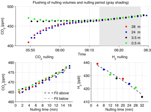
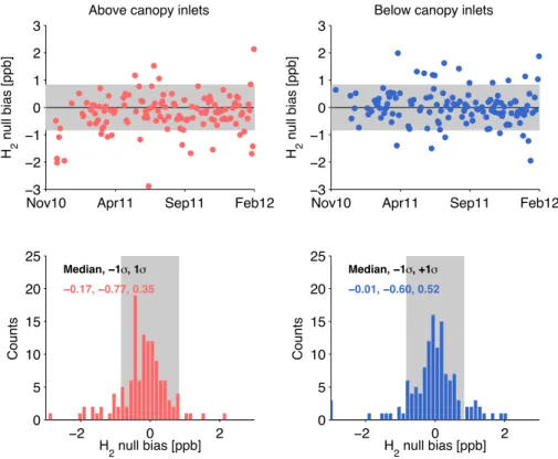
An example of our nulling procedure on the morning of 2 August 2011 (Fig. 4) shows
the transition of the CO2sampling system from tower measurements to the nulling
vol-ume as the integrating volvol-umes flushed. The null bias between inlet heights for each H2,
CO2, and H2O gradient pair was calculated after detrending with a second-order
poly-nomial to account for the drift in concentrations due to lower-frequency atmospheric
20
variability. In this example, the apparent null bias between the above (below) canopy
inlets was 1.06 (1.63) ppb and 0.92 (−0.33) ppm for H2and CO2, respectively. Over the
entire study period, the median H2 null bias was−0.17 and−0.01 ppb for the
above-and below-canopy gradient pairs, respectively, above-and was approximately normally
dis-tributed (1σ;−077 to 0.52) (Fig. 5). The observed null bias was smaller than the
com-25
bined analytical uncertainty (minimum detectable difference given instrument precision
√
2σ), so it was not possible to distinguish it from zero, and the H2 bias between the
AMTD
7, 2879–2928, 2014Ecosystem fluxes of hydrogen
L. K. Meredith et al.
Title Page
Abstract Introduction
Conclusions References
Tables Figures
◭ ◮
◭ ◮
Back Close
Full Screen / Esc
Printer-friendly Version Interactive Discussion
Discussion
P
a
per
|
D
iscussion
P
a
per
|
Discussion
P
a
per
|
Discuss
ion
P
a
per
|
The nulling procedure was a valuable tool to diagnose bias to between sampling lines, though in retrospect mixing the reservoir, increasing its volume, using multiple reservoirs in series, or filling the reservoir from a level with less variability (i.e., from above the canopy), to reduce concentration variability and drift over the nulling proce-dure would yield better data on the null bias.
5
3 Gradients and flux-gradient methods
In this section, we present mole fraction gradients measured at Harvard Forest. The theory and applicability of three flux-gradient methods is discussed and the filtering criteria are described.
3.1 Gradient measurements
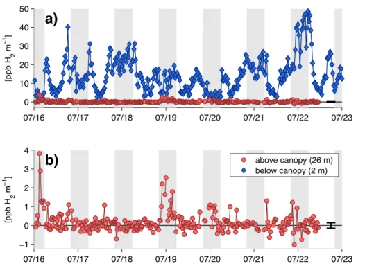
10
This study was the first application of the GC-HePDD to measure H2 gradients in
the field. We observed statistically significant H2 gradients both above and below the
canopy at Harvard Forest. H2 gradients were typically more than an order of
magni-tude larger below the forest canopy than above because of the reduced turbulence and
proximity to the H2sink close to the soil surface (Fig. 6). Gradients exhibited a diurnal
15
pattern with stronger gradients at night during calm atmospheric conditions when H2
lost to soil uptake was not replenished by H2 from above. The above-canopy H2
gra-dients were often close to the precision of the GC-HePDD system, especially during turbulent daytime periods. As a result, raw measurements were averaged to reveal the environmental gradients and fluxes, as has been previously required for these types of
20
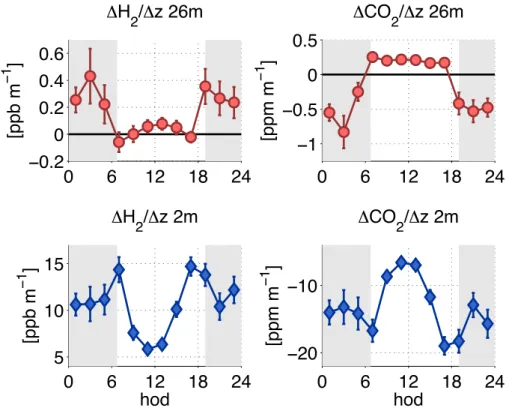
measurements above the forest canopy (Simpson et al., 1997). For example,
above-and below-canopy gradients of H2 and CO2 averaged into 2 h bins for the month of
July clearly showed the underlying environmental signal (Fig. 7). Soil uptake of H2led
to positive H2gradients above and below the forest canopy. Above-canopy CO2
gradi-ents oscillated from positive during the day when photosynthetic uptake of CO2by the
AMTD
7, 2879–2928, 2014Ecosystem fluxes of hydrogen
L. K. Meredith et al.
Title Page
Abstract Introduction
Conclusions References
Tables Figures
◭ ◮
◭ ◮
Back Close
Full Screen / Esc
Printer-friendly Version Interactive Discussion
Discussion
P
a
per
|
D
iscussion
P
a
per
|
Discussion
P
a
per
|
Discuss
ion
P
a
per
|
forest canopy was the dominant process to negative at night when ecosystem respira-tion was the overwhelming process. Respirarespira-tion was the dominant process below the
forest canopy, as indicated by consistently negative below-canopy gradients. CO2mole
fraction gradient measurements above and below the canopy agree well with
simulta-neous CO2 profile measurements at the EMS site (unpublished Harvard Forest EMS
5
data; Urbanski et al., 2007; Wehr et al., 2013).
Higher signal-to-noise ratios could have been achieved for H2 gradients measured
over a larger vertical height (∆z) difference. However, the above canopy 4 m ∆z was
limited by the height of the tower above the forest canopy. Close to the soil sink, below
canopy H2 gradients were well above instrument precision and the 3 m ∆z was suffi
-10
cient. For future studies, inlet heights below the canopy could be installed farther from
the soils (>0.5 m) and be place closer together (∆z <3 m), to still measure statistically
significant gradients that may be more linear than in our case. For studies with taller
towers above the vegetative canopy, a greater distance between the inlets (∆z >4 m)
could increase the mole fraction gradient signal-to-noise ratio, but should not exceed
15
relevant eddy length scales.
3.2 Flux-gradient methods
Flux-gradient methods were used to calculate the flux of a trace gas from the measured
gradient and a number of different parameters. In most presentations of flux-gradient
methods, an analogy is drawn to Fick’s first law for molecular diffusion, such that it
20
is directly or implicitly stated that conservative fluxes, FC1, of gas molecules (Eq. 1)
are equal to the product of their mole fraction gradient (∆C1/∆z) in the down-gradient
direction and the eddy diffusivity,K, which depends on the intensity of turbulent mixing
over time intervals appropriate to the scale of the process (Baldocchi et al., 1995; Goldstein et al., 1996; Goldstein, 1998; Dunn et al., 2009).
25
FC1=−K
∆C1
AMTD
7, 2879–2928, 2014Ecosystem fluxes of hydrogen
L. K. Meredith et al.
Title Page
Abstract Introduction
Conclusions References
Tables Figures
◭ ◮
◭ ◮
Back Close
Full Screen / Esc
Printer-friendly Version Interactive Discussion
Discussion
P
a
per
|
D
iscussion
P
a
per
|
Discussion
P
a
per
|
Discuss
ion
P
a
per
|
In this context,∆denotes the mean difference between 30 min measurements at each
level of a vertical gradient pair andρn is the molar density of air. The turbulent mixing
coefficientK is inferred or parameterized, unlike the molecular diffusion coefficient in
Fick’s first law that can be derived from first principles using molecular kinetic theory.
Flux-gradient methods assume that at a given time and place, the eddy diffusivity is
5
invariant for mass, heat, and momentum (e.g., Reynold’s Analogy) (Garratt and Hicks, 1973; Sinclair and Lemon, 1975; Baldocchi et al., 1988).
In general, to calculate trace gas fluxes, flux-gradient methods require that there are no sources or sinks of the trace gas or the reference species between the gradient inlets. This was not a problem in our study because gradient pairs were located either
10
above or below the forest canopy (Fig. 2), and whole-canopy gradients were only used when gas fluxes from the canopy should have been minimal. For the methods to work,
trace gas species should not have significantly different vertical distributions of sources
and sinks. Furthermore, the trace gas in question should be inert over the time scale of the flux-gradient measurement, meaning that the timescale of turbulence (200–300 s in
15
such ecosystems) should not exceed the time scale of chemical reactions (Baldocchi et al., 1988; Baldocchi and Meyers, 1991).
Flux-gradient theories have been found to overestimate scalar fluxes within the roughness sublayer, which is the region from the ground to two or three times canopy height because the turbulent structure is influenced (mechanically and thermally) by the
20
canopy elements (Raupach and Thom, 1981; Baldocchi and Meyers, 1988; Högström et al., 1989; Simpson et al., 1998) and over tall vegetation (Garratt, 1978). That said, the theory might be less compromised than previously thought above forests even at just 1.4 times the canopy height (Simpson et al., 1998). In our case, the tower height (30 m) constrained the height of the above canopy inlets, which were centered on
ap-25
proximately 1.2 times the canopy height within the roughness sublayer. We evaluated the performance of flux-gradient methods against independent flux measurements of
AMTD
7, 2879–2928, 2014Ecosystem fluxes of hydrogen
L. K. Meredith et al.
Title Page
Abstract Introduction
Conclusions References
Tables Figures
◭ ◮
◭ ◮
Back Close
Full Screen / Esc
Printer-friendly Version Interactive Discussion
Discussion
P
a
per
|
D
iscussion
P
a
per
|
Discussion
P
a
per
|
Discuss
ion
P
a
per
|
Below canopy environments are characterized by low wind speeds and intermittent turbulent events that can violate flux-gradient theory assumptions. Counter-gradient transport of heat, momentum, and trace gases has been documented beneath plant canopies and may severely compromise flux-gradient methods (Shaw, 1977; Raupach and Thom, 1981; Baldocchi and Meyers, 1988; Amiro, 1990; Baldocchi and Meyers,
5
1991). On the other hand, flux-gradient methods have been preferred over eddy co-variance techniques for measuring surface–atmosphere fluxes within a few meters of the surface layer (Fitzjarrald and Lenschow, 1983; Gao et al., 1991; de Arellano and Duynkerke, 1992; Wagner-Riddle et al., 1996; Taylor et al., 1999; Dunn et al., 2009). Intermittent turbulent transport events may become less important near the ground,
10
where the sources or sinks of tracers can be large; therefore, Meyer et al. (1996) argue that near the forest floor the flux-gradient relationships are valid and their application is justified.
The availability of different parameters, and the applicability of a given flux-gradient
method varied with time and location in our experiment (Table 1). Whole canopy fluxes
15
could not be calculated during the growing season daytime because of canopy in-terference. The sensible heat flux method was only applied outside the 2011 grow-ing season because the fans in the aspirated temperature shields were damaged by a lightning strike on 28 May 2011, which was not apparent from the data, and was
only discovered six months later. In this study, we determined H2 fluxes using three
20
different flux-gradient methods: trace gas similarity, sensible heat (H) similarity, andK
parameterization.
3.2.1 Trace gas similarity
The first method, trace gas similarity, assumes similarity of H2fluxes and gradients to
CO2 or H2O flux-gradients that can be measured by an independent method and is
25
often referred to as a Modified Bowen Ratio technique. The flux (FC1) of a given trace
gas is calculated from its mole fraction gradient (∆C1/∆z) and measurements of the
AMTD
7, 2879–2928, 2014Ecosystem fluxes of hydrogen
L. K. Meredith et al.
Title Page
Abstract Introduction
Conclusions References
Tables Figures
◭ ◮
◭ ◮
Back Close
Full Screen / Esc
Printer-friendly Version Interactive Discussion
Discussion
P
a
per
|
D
iscussion
P
a
per
|
Discussion
P
a
per
|
Discuss
ion
P
a
per
|
et al., 1996; Goldstein et al., 1996, 1998; Lindberg and Meyers, 2001).
FC1=FC2
∆C1
∆C2
(2)
The trace gas eddy diffusion coefficients (K) for CO2 and H2O were compared (R
2
=
0.68, slope=1.07) at Harvard Forest in the past (Goldstein et al., 1996). However, it
5
is important to note that the idea of similarity applied in this method is more general
than diffusional theory and calculation of K. Trace gas similarity only assumes linear
transport of trace gases considered to be inert over the spatial and temporal scale of the measurement and that have a similar spatial distribution of sources and sinks. The
method is therefore more general than is often attributed to flux-gradient methods.K is
10
not calculated explicitly by similarity methods. These points also apply to the sensible heat similarity method.
Independent flux measurements of CO2 and H2O via eddy covariance and of CO2
via automated flux chambers were available above and below the forest canopy, re-spectively. In this study, the trace gas similarity method was applied both above and
15
below the canopy all year round and to the whole canopy gradient outside the growing season as data availability allowed.
3.2.2 Sensible heat similarity
The second method, sensible heat similarity, assumes similarity of H2 fluxes and
gra-dients to the sensible heat flux and temperature gradient (Meyers et al., 1996; Liu and
20
Foken, 2001; Dunn et al., 2009). The sensible heat flux (H) and temperature gradient
(∆T/∆z) are related by the turbulent transfer coefficient for heatKH(Businger, 1986),
H=−KH∆ T
∆zρmcp (3)
whereρmis the mass density of air andcpis the specific heat capacity of air. Following
25
AMTD
7, 2879–2928, 2014Ecosystem fluxes of hydrogen
L. K. Meredith et al.
Title Page
Abstract Introduction
Conclusions References
Tables Figures
◭ ◮
◭ ◮
Back Close
Full Screen / Esc
Printer-friendly Version Interactive Discussion
Discussion
P
a
per
|
D
iscussion
P
a
per
|
Discussion
P
a
per
|
Discuss
ion
P
a
per
|
applying a water vapor correction to the buoyancy flux derived from sonic anemometer temperature measurements, and the crosswind term is neglected because it should be small compared to the other terms,
H= hw
′T′
si ∆T
∆z +0.51T
∆q
∆z
×∆T
∆z ×ρm×cp (4)
5
Here hw′Ts′i is the sonic heat flux and q represents the water vapor mole fraction.
Equation 4 gives the flux-gradient form (Eq. 1) for sensible heat, which can then be
used to determine the H2flux (Eq. 5) by inferringKH.
FC1=H×
∆C1
∆T × ρn ρmcp
(5)
10
The eddy diffusion coefficients (K and KH) for trace gases and heat were measured
at Harvard Forest in the past, agreeing within 12±10 % when compared to both H2O
and CO2 (Goldstein et al., 1996). The method has been applied to determine
hydro-carbon fluxes above a forest canopy (Goldstein et al., 1996) and the specific method
adopted in our study was developed for the calculation of CO2 and H2O fluxes close
15
to the ground (Dunn et al., 2009). This is a modified Bowen ratio (MBR) technique (Liu and Foken, 2001) that can be used to determine sensible (and latent heat) fluxes (errors of less than 10 %) and it circumvents errors (often on the order of 20–30 %) associated with methods that require closure of the measured surface energy bud-get, such as the Modified Bowen Ratio Energy Balance (MREB) method (Sinclair and
20
Lemon, 1975; Baldocchi et al., 1988; Liu and Foken, 2001 and references therein). In
previous work, H2 fluxes were determined using the MREB method over grassland in
Quebec (Constant et al., 2008). In this study, the sensible heat similarity method was applied below the canopy during months when the aspirated temperature shields were functioning (November 2010 to May 2011 and December 2012 to March 2012).
AMTD
7, 2879–2928, 2014Ecosystem fluxes of hydrogen
L. K. Meredith et al.
Title Page
Abstract Introduction
Conclusions References
Tables Figures
◭ ◮
◭ ◮
Back Close
Full Screen / Esc
Printer-friendly Version Interactive Discussion
Discussion
P
a
per
|
D
iscussion
P
a
per
|
Discussion
P
a
per
|
Discuss
ion
P
a
per
|
3.2.3 K parameterization
The third method, K parameterization, invokes Monin–Obukhov similarity theory to
parameterize a turbulent exchange coefficient (K) from sonic anemometer
measure-ments, and is often referred to as an aerodynamic method (Monin and Obukhov, 1954;
Simpson et al., 1998). K can be estimated by a variety of aerodynamic methods
de-5
rived from energy or momentum balances (Högström et al., 1989; Celier and Brunet,
1992; Simpson et al., 1998; Foken, 2006). For example,K can be determined from
K=u
∗k(z−d)
φm
(6)
Here,u∗is the friction velocity (a characteristic velocity scale calculated from the square
10
root of covariance between vertical and horizontal wind),k is von Karman’s constant
(taken as 0.4),z is the height above the ground, andd is the zero-plane displacement
height, andφm is the diabatic influence function for momentum (Monin and Obukhov,
1954; Simpson et al., 1998). The Monin-Obukhov length (L=kgu∗3
T H
ρmcp
) is used to
deter-mineφmfrom the empirical descriptions outlined by Eqs. 22a and 22b in Foken, 2006.
15
The method has been applied close to the surface (Fritsche et al., 2008) and above the
forest canopy (Simpson et al., 1997; Simpson et al., 1998). In this study, theK
param-eterization method was applied below the canopy. Assuming thatz=2 m (the height
of theu∗measurement), the displacement height was inferred empirically to be around
1.63 m (z−d=0.37 m) by comparing the parameterized K to that determined using
20
Eq. (2) using chamber fluxes and concentration gradients. The determination ofd is
often problematic (Raupach and Thom, 1981). Physically,d represents an adjustment
of the basis height to reflect the displacement by the surface features of the profiles
of micrometeorological variables fundamental to theK parameterization at hand. The
inferred value for d was consistent throughout the study period and may reflect the
25
AMTD
7, 2879–2928, 2014Ecosystem fluxes of hydrogen
L. K. Meredith et al.
Title Page
Abstract Introduction
Conclusions References
Tables Figures
◭ ◮
◭ ◮
Back Close
Full Screen / Esc
Printer-friendly Version Interactive Discussion
Discussion
P
a
per
|
D
iscussion
P
a
per
|
Discussion
P
a
per
|
Discuss
ion
P
a
per
|
3.3 Data filtering
Data were filtered to reject unrealistic values and to appropriately apply flux-gradient methodology. By their nature, the trace gas similarity and sensible heat similarity meth-ods are not valid when the gradient of the comparative species (Eqs. 2 and 5, de-nominator) approaches zero or changes sign over the measurement period. Similarity
5
method cannot work during such periods, so we limited flux calculations to periods when gradients in the denominator were above their measurement precision. In gen-eral, the fluxes calculated during dawn and dusk periods are not included in averages or comparative assessments because of the tendency for conditions to change such that the observed fluxes and gradients provide no information about the turbulence.
10
For example, conditions pass through an isothermal point when air and surfaces have the same temperature so there is no gradient driving a heat flux, when air is saturated
there is no gradient driving a water vapor flux, and when photosynthesis ceases CO2
gradients change sign.
Data were rejected during rainy periods with more than 0.2 mm of rain per 30 min
15
(Baldocchi and Meyers, 1991). Periods with u∗<0.07 m s−1 and u∗<0.17 m s−1 were
excluded for below and above canopy data, respectively, because of poorly developed turbulent conditions (Goulden et al., 1996; Liu and Foken, 2001; Bocquet et al., 2011) and potential for advective fluxes driven by drainage flows on sloping terrain (Yi et al.,
2008). We excluded unrealistic values of the implied turbulent transfer coefficients,
20
K, such that 0≤K ≤0.5 m2s−1 and 0≤K ≤5 m2s−1 for the below-canopy and the
whole-/above-canopy fluxes, respectively. We did not filter based on the wind sector because we found no interference from the tower and instrument shed to the east (45
to 180◦). We considered quantile-quantile plots of the residual between flux-gradient
methods and eddy covariance fluxes, and excluded clear outliers: residual absolute
25
values>20 µmol m−2s−1and>10 mmol m−2s−1for CO2and H2O fluxes. Additional
fil-ters were applied to the sensible heat flux method to retain only reasonable sonic and sensible heat flux values:|< w′Ts′>|<0.1 K m s−
1
AMTD
7, 2879–2928, 2014Ecosystem fluxes of hydrogen
L. K. Meredith et al.
Title Page
Abstract Introduction
Conclusions References
Tables Figures
◭ ◮
◭ ◮
Back Close
Full Screen / Esc
Printer-friendly Version Interactive Discussion
Discussion
P
a
per
|
D
iscussion
P
a
per
|
Discussion
P
a
per
|
Discuss
ion
P
a
per
|
data were excluded when the temperature gradient was greater than 0◦C at the same
time asH was greater than 3 W m−2, which occurred at sunrise and sunset because of
the rapidly changing conditions over the 30 min averaging interval (Meyers et al., 1996; Dunn et al., 2006).
Filtering is known to result in a large amount of rejected data in flux-gradient methods
5
(e.g., net 57 % data loss in detailed analysis by Bocquet et al., 2011). Conditions at the site, external to the measurement system, resulted in a 13 %, 19 %, and 6 % loss
of data based on the 29 mu∗, 2 m u∗, and precipitation filter criteria. Filtering criteria
related to the flux methods resulted in a raw data loss over the experimental period of around 40–62 % for trace gas similarity, 87 % for sensible heat similarity, and 18–26 %
10
forK parameterization.
4 Flux-gradient methods: evaluation and application
Using independent flux measurements of CO2and H2O derived from eddy covariance
and chamber techniques we produced a quantitative guide (Table 2) for the
perfor-mance of each flux-gradient method (trace gas similarity, sensible heat similarity, andK
15
parameterization) at each measurement location (above-, whole-, or below-canopy) for
different seasons and times of day. We compared measurements during summer (23
June 2011 to 16 October 2011) and winter (15 November 2011 to 28 February 2012) during day- (10:00–16:00) and night-time (21:00–05:00) periods. We assign a perfor-mance flag of good, fair, or poor based on the statistical tests described in Table 2 and
20
AMTD
7, 2879–2928, 2014Ecosystem fluxes of hydrogen
L. K. Meredith et al.
Title Page
Abstract Introduction
Conclusions References
Tables Figures
◭ ◮
◭ ◮
Back Close
Full Screen / Esc
Printer-friendly Version Interactive Discussion
Discussion
P
a
per
|
D
iscussion
P
a
per
|
Discussion
P
a
per
|
Discuss
ion
P
a
per
|
4.1 Comparing eddy covariance and chamber CO2flux measurements
We assessed the consistency between the independent eddy covariance and
cham-ber CO2flux data to defend their use to then evaluate the flux-gradient methods. Eddy
covariance measurements represent the whole ecosystem flux and chamber
measure-ments just the soil flux. Studies comparing nocturnal CO2eddy flux with chamber
mea-5
surements often report significant discrepancies of 20 to over 50 % (e.g., Goulden et al., 1996; Lavigne et al., 1997; Phillips et al., 2010). We did not expect exact agreement be-tween eddy and chamber fluxes because of the mismatch in measurement footprints, but expected to see fluxes of a comparable magnitude with similar diel patterns.
The relevant eddy-derived quantity to compare to surface-based chamber
measure-10
ments is the u∗-filtered (Sect. 3.3) nocturnal net ecosystem exchange (NEE), which
accounts for the time lag between CO2emitted by respiration and its release from
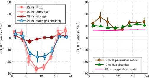
stor-age from beneath the canopy (storstor-age in the sense of Wofsy et al., 1993). The mean chamber flux was approximately two times higher than NEE at night over the weeklong summer example period (Fig. 8) and the diel chamber fluxes were about 50 % higher
15
than a simple ecosystem respiration model (Urbanski et al., 2007). Nocturnal chamber
and NEE CO2fluxes were correlated over the whole study period with a nonzero bias
(r=0.42∗, bias=−0.2 µmol m−2s−1) and had fair agreement in the summer and winter
periods, but poor daytime winter performance (Table 2). Chamber measurements
over-estimated CO2fluxes relative to NEE in the summer (26 % bias), and underestimated
20
them in the winter (−50 % bias) (Table 2). The summer bias estimate does not include
respiration from canopy elements (woody tissue and foliage), which can contribute up to 50 % of the total ecosystem respiration, but usually less than 20 % (Goulden et al., 1993; Lavigne et al., 1997; Davidson et al., 2002). Therefore, summertime chamber plus canopy respiration was likely at least 46 % higher than the NEE estimates in the
25
AMTD
7, 2879–2928, 2014Ecosystem fluxes of hydrogen
L. K. Meredith et al.
Title Page
Abstract Introduction
Conclusions References
Tables Figures
◭ ◮
◭ ◮
Back Close
Full Screen / Esc
Printer-friendly Version Interactive Discussion
Discussion
P
a
per
|
D
iscussion
P
a
per
|
Discussion
P
a
per
|
Discuss
ion
P
a
per
|
south (Goulden et al., 1996). In spite of this offset, chamber fluxes and NEE were
sig-nificantly correlated, which gave us confidence that the independent data sets both
contained information on ecosystem fluxes of CO2 that could be used to evaluate the
flux-gradient methods.
4.2 Flux-gradient method evaluation
5
We evaluated the performance of the flux-gradient methods against independent CO2
(eddy covariance and chamber) and H2O (eddy covariance) flux measurements for
summer and winter periods (Table 2). The seasonal trends are illustrated by week-long periods from the summer (15–22 July 2011 period) and winter (1–14 February 2012) in Figs. 8 and 9, respectively. The trace gas similarity method above the forest canopy
10
(Sect. 3.2.2; 26 m) reproduced the diel cycle measured via eddy covariance in both
the summer (Fig. 8 for CO2 and Fig. A1 for H2O) and winter (Fig. 9), as was reflected
by the significant correlations between the measurements (Table 2). Only the trace gas
similarity H2O flux on winter days had poor performance, which may have been caused
by the low signal-to-noise of concentration gradients in the turbulent above canopy
en-15
vironment when water vapor fluxes were low. The trace gas similarity method showed
good performance for both CO2 and H2O during the day above the forest canopy in
the summer period (Table 2) and for the whole measurement period (CO2: r=0.85∗,
bias=0.69 µmol m−2s−1; H2O,r=0.71∗, bias=0.57 mmol m−
2
s−1). The above canopy
trace gas similarity method systematically underestimated CO2 fluxes and
overesti-20
mated H2O fluxes, despite the agreement of the mole fraction measurements between
the EMS system and this study (Sect. 2.3). This difference could be translated to the
inferredK values (Eq. 1), andKH2O=0.68×KCO2 (R
2
=0.51). This result indicated the
turbulent eddy diffusivity was not invariant for CO2 and H2O above the forest canopy
as was assumed in the trace gas similarity method. The cause could be the different
25
distribution of sources and sinks of the two trace gases. CO2 and H2O both have
AMTD
7, 2879–2928, 2014Ecosystem fluxes of hydrogen
L. K. Meredith et al.
Title Page
Abstract Introduction
Conclusions References
Tables Figures
◭ ◮
◭ ◮
Back Close
Full Screen / Esc
Printer-friendly Version Interactive Discussion
Discussion
P
a
per
|
D
iscussion
P
a
per
|
Discussion
P
a
per
|
Discuss
ion
P
a
per
|
source was stronger relative to the above canopy fluxes than the H2O soil source (e.g.,
four-fold greater in the case of Fig. 8 vs. Fig. A1) and is of opposite sign.
The whole canopy trace gas similarity method (Sect. 3.2.2; centered on 10 m) could only be applied in the absence of interfering canopy sources or sinks between the gradient inlets (24 m and 3.5 m), making this method more restricted in its application
5
than the above canopy method. However, we found that the whole canopy method was
a superior method in some cases when trace gas gradients were small and difficult
to detect above the forest canopy, such as during the winter and at night (Table 2).
For example, day- and winter-time H2O fluxes from whole canopy trace gas similarity
using CO2as the correlative variable were good, while that method applied above the
10
canopy had poor performance (Table 2). An example of the 10 m trace gas similarity
CO2fluxes is shown in Fig. 9.
CO2 fluxes calculated by the sensible heat similarity method (Sect. 3.2.2; 2 m) were
significantly correlated with chamber measurements all year (daytime:r =0.67∗, bias=
1.1 µmol m−2s−1), but tended to overestimate daytime fluxes (Table 2). The method was
15
only available during the wintertime, when heat fluxes and temperature gradients were small, which contributed to higher uncertainty in the results than for the other methods, as shown in Fig. 9. Agreement of the wintertime sensible heat similarity and eddy flux data across the forest canopy was poor to fair (Table 2).
The performance of the K parameterization method below the forest canopy
20
(Sect. 3.2.4; 2 m) vs. chamber measurements was good throughout the year (daytime:
r=0.74∗, bias=−0.12 µmol m−2s−1). These fluxes were significantly correlated with
chamber data and bias was low or insignificant (Table 2).K parameterization fluxes
were correlated with eddy covariance fluxes in most cases, but typically were biased positively in the summer and negatively in the winter as can be seen from the
com-25
parison with the NEE-derived simple ecosystem respiration model in Figs. 8 and 9.
The overestimation of nocturnal summertime fluxes by K parameterization was likely
related to the large and nonlinear CO2 gradients (determined from profile
AMTD
7, 2879–2928, 2014Ecosystem fluxes of hydrogen
L. K. Meredith et al.
Title Page
Abstract Introduction
Conclusions References
Tables Figures
◭ ◮
◭ ◮
Back Close
Full Screen / Esc
Printer-friendly Version Interactive Discussion
Discussion
P
a
per
|
D
iscussion
P
a
per
|
Discussion
P
a
per
|
Discuss
ion
P
a
per
|
heat similarity methods use ratios of vertical mole fraction or temperature gradients,
which can compensate for nonlinear vertical concentration gradients. The K
param-eterization has been shown to agree with trace gas similarity and eddy covariance-derived fluxes in the past (Fritsche et al., 2008). A larger period of overlapping data
for the sensible heat similarity method was available withK parameterization results
5
than chamber data, and the two flux-gradient methods were highly correlated, but had
a relative positive bias of the CO2 flux by the sensible heat method vs. K
parameter-ization over the whole period (dayr =0.63∗, bias=0.37 µmol m−2s−1; night r=0.42∗,
bias=0.11 µmol m−2s−1).
4.3 Flux-gradient method application: H2gradient fluxes 10
The flux-gradient methods were used to calculate fluxes of H2 above and below the
canopy, for which no independent eddy or chamber measurements were available.
Summertime H2 fluxes were calculated for the 15–22 July 2011 period above the
canopy by the trace gas similarity methods using the CO2 and H2O eddy fluxes, and
below the canopy from trace gas similarity to CO2using CO2chamber measurements
15
and as well as theK parameterization method (Fig. 10). The H2 fluxes were
charac-terized by net ecosystem H2 uptake and were consistent with our expectation that H2
uptake by soil would be the dominant ecosystem process. The below-canopy fluxes
were−8 nmol m−2s−1 and −10 nmol m−2s−1 during midday over this period for theK
parameterization and chamber-based trace gas similarity methods, respectively. The
20
above canopy trace gas similarity average midday H2 fluxes via CO2 and H2O were
−21 nmol m−2s−1 and −15 nmol m−2s−1, respectively. As was observed in Sect. 4.3,
larger trace gas fluxes were calculated using CO2as the correlative variable than H2O,
but in the case of H2this difference (and the difference with the below canopy fluxes)
fell within the 95 % confidence intervals because of the higher uncertainty in H2
gradi-25
ents measurements above the canopy. Storage fluxes of H2were calculated, but were