Estimates of eddy turbulence consistent with seasonal variations of atomic oxygen and its possible role in the seasonal cycle of mesopause temperature

www.ann-geophys.net/28/2103/2010/ doi:10.5194/angeo-28-2103-2010

© Author(s) 2010. CC Attribution 3.0 License.

Annales

Geophysicae

Estimates of eddy turbulence consistent with seasonal variations of

atomic oxygen and its possible role in the seasonal cycle of

mesopause temperature

M. N. Vlasov and M. C. Kelley

School of Electrical and Computer Engineering, Cornell University, Ithaca, NY, USA

Received: 5 April 2010 – Revised: 18 October 2010 – Accepted: 19 October 2010 – Published: 18 November 2010

Abstract. According to current understanding, adiabatic cooling and heating induced by the meridional circulation driven by gravity waves is the major process for the cold summer and warm winter polar upper mesosphere. However, our calculations show that the upward/downward motion needed for adiabatic cooling/heating of the summer/winter polar mesopause simultaneously induces a seasonal variation in both the O maximum density and the altitude of the [O] peak that is opposite to the observed variables generalized by the MSISE-90 model. It is usually accepted that eddy tur-bulence can produce the [O] seasonal variations. Using this approach, we can infer the eddy diffusion coefficient for the different seasons. Taking these results and experimental data on the eddy diffusion coefficient, we consider in detail and estimate the heating and cooling caused by eddy turbulence in the summer and winter polar upper mesosphere. The sea-sonal variations of these processes are similar to the seasea-sonal variations of the temperature and mesopause. These results lead to the conclusion that heating/cooling by eddy turbu-lence is an important component in the energy budget and that adiabatic cooling/heating induced by upward/downward motion cannot dominate in the mesopause region. Our study shows that the impact of the dynamic process, induced by gravity waves, on [O] distributions must be included in mod-els of thermal balance in the upper mesosphere and lower thermosphere (MLT) for a consistent description because (a) the [O] distribution is very sensitive to dynamic processes, and (b) atomic oxygen plays a very important role in chem-ical heating and infrared cooling in the MLT. To our knowl-edge, this is the first attempt to consider this aspect of the problem.

Keywords. Meteorology and atmospheric dynamics (Gen-eral circulation; Middle atmosphere dynamics; Turbulence)

Correspondence to:M. C. Kelley (mck13@cornell.edu)

1 Introduction and background

The thermal balance of the mesosphere and lower thermo-sphere (MLT) is controlled by radiative heating due to ab-sorption of solar UV radiation by O2 and O3, by chemical

heating from exothermic reactions, by radiative cooling asso-ciated with infrared emission of CO2, and heating and

cool-ing induced by dynamic processes. The latter includes com-pression/expansion caused by downward/upward motion as-sociated with the gravity wave-driven meridional circulation, as well as direct heating due to the gravity wave dissipation and turbulent diffusion from breaking gravity waves and/or the Kelvin–Helmholtz instability (KHI), caused by sheared flow.

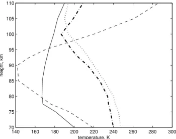
140 160 180 200 220 240 260 280 300 70

75 80 85 90 95 100 105 110

temperature, K

height, km

Fig. 1. Temperature height profiles calculated by the MSISE-90 model (14:00 LT, 21 December 2000, Long. = 285◦E) at 70◦S lat-itude in the summer cold mesosphere (dashed line) and at 70◦N latitude in the winter warm mesosphere (dashed-dotted line), and as calculated by the SOCRATES model at the same latitudes in sum-mer (solid line) and in winter (dotted line).

important (Berger and von Zahn, 1999). As seen from Fig. 1, agreement exists between the height profiles of the temper-ature calculated by the model and given by the MSISE-90 model (Hedin, 1991) at altitudes below the polar win-ter mesopause, but the model and the MSISE-90 data are very different above the mesopause. The agreement be-tween the SOCRATES and MSISE-90 models is much worse around the polar summer mesopause. The strong discrep-ancies between the SOCRATES models and the empirical model MSISE-90 are as follows:

1. The SOCRATES model cannot reproduce one of the main features of the mesosphere-lower thermosphere (MLT): the decrease in the lower boundary of the ther-mosphere from winter to summer. It is very difficult to believe that the lower boundary of the thermosphere is located below 80 km in summer, as seen in Fig. 1. 2. In Fig. 2, a strong discrepancy exists between the

cal-culated temperatures and the temperatures given by the MSISE-90 model at middle latitudes.

3. According to the MSISE-90 model, the latitudinal vari-ation of temperature at the winter mesopause does not exceed 8 K, but this variation is 38 K in the summer mesopause. Also, the MSISE-90 model (see Fig. 3) shows that the maximum decrease in temperature at the summer polar mesosphere from winter solstice to equinox is about 50 K but the maximum increase in temperature in the winter mesosphere is 20 K (also see Fig. 3). A mechanism based on adiabatic

heat-170 180 190 200 210 220 230 240 250 70

75 80 85 90 95 100 105 110

temperature, K

height, km

Fig. 2.The same as in Fig. 1 but at latitudes 40◦N and 40◦S.

100 150 200 250 300 350 400 70

75 80 85 90 95 100 105 110 115 120

temperature, K

height, km

S W

Fig. 3.Temperature height profiles given by the MSISE-90 model at latitudes 70◦S and 70◦N (curves labeled S and W, respectively), at the equator (dotted curve), at winter solstice (14:00 LT, 21 Decem-ber 2000, Long. = 285◦E), and at latitudes 70◦S and 70◦N (dashed and solid curves, respectively) at equinox.

ing/cooling cannot explain these asymmetries between the summer and winter mesosphere.

We note also that the SOCRATES results strongly contradict the heating rate of +10 to +20 K/day determined by (a) in situ measurements of neutral density fluctuations in the sum-mer polar mesopause (L¨ubken, 1997), and (b) the dynamic cooling rate of−31 K/day associated with the vertical heat transport by dissipating gravity waves in the mesopause re-gion as measured by a Na lidar at the Starfire Optical Range in winter at middle latitudes (Gardner and Yang, 1998).

structure at high latitudes. Dynamic forcing is provided by gravity wave energy and momentum fluxes and their diver-gences. The model gives a turbulent heating rate of +20 to +25 K/day in the summer polar mesopause that increases with increasing altitude, reaching 60 K/day at 100 km. This high heating requires an upward velocity of 5 cm/s to provide net adiabatic cooling in the summer mesopause.

The Fritts and Luo (1995) model shows that eddy turbu-lence and vertical motion induced by gravity waves play a very important role in the thermal balance in the upper meso-sphere. Gardner and Yang (1998) also showed the impor-tance of gravity wave dissipation in thermal balance in the upper mesosphere.

However, Smith (2004), Hocking (1999), and other au-thors (for example, Brasseur and Solomon, 1986; Brasseur et al., 2000) argue that the impact of gravity waves is restricted to their induced change in the zonal and meridional wind and, correspondingly, to adiabatic heating/cooling induced by the downward/upward motion and that this is the main source of the temperature seasonal variations in the upper mesosphere. Hocking (1999) and Smith (2004) do emphasize many un-certainties in the relationship of turbulent energy dissipation, turbulent heat transport, and diffusion. Hocking notes two main problems: “first, turbulence is very intermittent both temporally and spatially, and very often occurs in thin layers in the middle atmosphere. These thin layers are often sepa-rated by regions that are either only weakly turbulent or even laminar. Secondly, the processes which induce diffusion can themselves be scale dependent.” These problems are very important when describing short-time variations in the tem-perature. However, when we try to model such long-time seasonal variations, we need mean values for the statistically steady turbulent motion. Numerous experimental data on eddy turbulence exist (see, for example, Fukao et al., 1994; L¨ubken, 1997; Hill et al., 1999), and these data facilitate in-ferring the mean values of eddy turbulence and their long-time seasonal variations. It is important to emphasize that the meridional wind and wind shears are very intermittent in altitude, as can be seen from the measurements (Larsen, 2002), meaning that vertical motion driven by the meridional wind is very intermittent as well. Finally, no available mea-surements of the vertical velocity exist, and estimates of this velocity from divergence of the horizontal wind are very dif-ficult. However, there are many measurements of the eddy diffusion coefficient.

Several approaches to estimating the heating rates cor-responding to turbulent dissipation of gravity wave kinetic energy were developed recently (Medvedev and Klaassen, 2003; Becker, 2004; Akmaev, 2007; Becker and McLan-dress, 2009). The heating rates estimated by Becker (2004) for summer conditions are similar to the heating rates mea-sured by L¨ubken (1997), but Becker’s peak value is less by a factor of about 2 and the peak height is smaller by 7 km than L¨ubken’s measured parameters. However, the estimated heating rates for winter conditions are very different from the

measured values. There are similar differences between the eddy diffusion coefficients calculated by Becker (2004) and measured by L¨ubken (1997). Akmaev (2001) simulated an eddy diffusion coefficient peak altitude of 110 km for Jan-uary that is higher by 17 km than the peak altitude measured by L¨ubken (1997).

To our knowledge, the models explaining the cold summer and warm winter mesopause do not consider the effect of dy-namic processes on the distribution of atomic oxygen, which plays an important role in chemical heating and infrared cooling in the upper mesosphere. For example, the extended version of the Canadian Middle Atmosphere Model pre-sented by Fomichev et al. (2002) includes eddy and molecu-lar diffusion and vertical advection, which strongly influence the [O] distribution. However, the model uses vertical pro-files for [O] given by the MSISE-90 model. The infrared radiation of the 15-µm CO2band is the main cooling process

in the upper mesosphere. The quenching of excited CO2by

atomic oxygen is one of the most important factors determin-ing this cooldetermin-ing. The authors tried to reduce the cooldetermin-ing rate error below 5% in the upper mesosphere. However, the vari-ations in atomic oxygen, induced by the dynamic processes included in the model, can change this cooling rate by a few times. Note that atomic oxygen is the main constituent in the thermosphere and that the O thermospheric density strongly depends on the altitude of the peak density in the upper meso-sphere. The altitude of the peak density is controlled by the dynamic processes responsible for the temperature anomaly in the mesopause.

The goal of this paper is to consider the contradiction between the observed seasonal variations of atomic oxy-gen density distributions in the upper mesosphere and lower thermosphere (MLT) and the impact of upward/downward motion, responsible for the cold summer and warm winter mesopause, on the [O] distribution. We estimate the impact of eddy turbulence and vertical motion on the [O] distribu-tions, derive the eddy diffusion coefficient corresponding to the seasonal variations of [O] corresponding to the exper-imental data associated with the MSISE-90 model (Hedin, 1991), and then, using these results, estimate the contribu-tion of heating/cooling of eddy turbulence in the thermal bal-ance of the upper mesosphere and the seasonal variations of mesopause temperature. To our knowledge, this is the first attempt to include a minor constituent in testing theories for the cold summer and warm winter mesopause.

2 Impact of eddy diffusion and vertical motion on the [O] distribution

0 50 100 150 200 250 0

0.5 1 1.5 2 2.5 3 3.5

4x 10

11

height, 0.1km

[O], cm−3

1 2

3 4

5 6

Fig. 4. [O] height profiles calculated by the analytical solution of Eq. (8) above 90 km forK_edm=3×106cm2/s and vertical velocities

V=2, 3, 4 cm/s (curves 1, 2, and 3, respectively), and forK_edm= 2×106cm2/s andV=2, 3, 4 cm/s (curves 4, 5, and 6, respectively).

photochemistry, on the [O] distribution in the MLT. Accord-ing to their results, the O peak density decreases with aKed

increase. This density decreases even more if a downward motion occurs with eddy turbulence. Also, the altitude of the [O] peak decreases with aKedincrease, whereas this

al-titude increases/decreases due to any upward/downward mo-tion. The seasonal variations of the O peak density and the altitude of the [O] peak are characterized by an increase in both the O peak density and the altitude of the [O] peak from summer to winter by a factor of nearly 2.25 and by 4 km, respectively.

The height distribution of the O density can be determined using the continuity equation,

∂n ∂z

−Ked(z)

_∂n

∂z+

n H

−D

_∂n

∂z+

n

HO

+V (z)n

=q(z)−β(z)n2 (1)

whereDis the molecular diffusion coefficient,V is the ve-locity,q is the production rate,βis the recombination coef-ficient, andHOis the height scale of atomic oxygen.

The solution of this equation, with constant values ofV,

Ked≫D,q=q0exp(−z/H ), and β=β0= constant in the

final termβ0n, is given by the formula

n=n0−

_q

0H

β0H−V

exp

−0.5

1

H−

V

Ked

−

"

0.25

1

H−

V

Ked

2

+β0/Ked

#0.5 

z  

+ q0H

β0H−V

exp(−z/H ) (2)

0 1 2 3 4 5 6

x 1011 80

85 90 95 100 105 110 115

[O], cm−3

height, km

Fig. 5.The calculated [O] height distributions (dashed lines) given by the MSISE-90 model (solid lines) for summer (low densities) and winter (high densities) at latitudes 60◦N and 60◦S on 21 De-cember 2000.

This simple approximation describes the main features that impact the [O] height distribution: production, loss, and dy-namic processes (eddy turbulence and upward motion). As seen from Fig. 4, an increase in the upward velocity induces an increase in the O density and in the altitude of the [O] peak. AKed increase induces an [O] decrease. The effect

3 Heating and cooling by eddy turbulence

There are different approaches and numerical models for estimating the heating/cooling rates induced by the grav-ity waves in MLT (Medvedev and Klaassen, 2003; Becker, 2004; Akmaev, 2007, 2009; Becker and McLandress, 2009). All models start from gravity waves and then calculate the heating/cooling corresponding to the different dynamic pro-cesses induced and driven by gravity waves. Some models estimate the eddy diffusion coefficient, as mentioned in the introduction. However, we start from the eddy diffusion co-efficients and try to estimate the heating/cooling rates corre-sponding to them.

In this case, the heating/cooling rate of eddy turbulence is given by the formula (see Fritts and Luo, 1995)

Qed=

∂ ∂z

KecCpρ

_∂T

∂z+

g

Cp

+Kecρ

g T c

_∂T

∂z+

g

Cp

,(3)

whereKecis the eddy heat conductivity,ρis the undisturbed

gas density,gis the gravitational acceleration,T is the tem-perature,Cpis the specific heat at constant pressure, andcis a dimensionless constant commonly taken to be 0.8 (L¨ubken, 1997; Hocking, 1999). The first term on the right side of Eq. (3) is the heat flux divergence, and the second term is the turbulent energy dissipation rate initiated by the dynamic in-stability of gravity waves and the action of viscous and buoy-ancy forces. For example, the first term presents divergence of heat flux corresponding to the heat flux given by Becker (2004) forPreff=1 and the heat flux given by formula (23)

in Akmaev (2007). The second term is similar to the total wave energy disposition rate per unit mass,ε=Kω2_B(1+P ), given by Akmaev (2007) whereP may be considered a gen-eralized Prandtl number andω2_B is the buoyancy frequency (Akmaev, 2007). There is great debate about the value of the turbulent Prandtl number. First of all, this problem is due to different assumptions about gravity wave energy transport and dissipation and localized or uniform induced turbulence. However, this problem is not within the scope of this paper. We restrict our calculations to only different values ofc.

Around the mesopause, the temperature gradient is small and∂Kec/∂zis small for theKecpeak in the mesopause. In

this case, Eq. (3) can be simplified to the formula

Qed=Kecg

∂ρ

∂z+Kecρ

g2

CpT c

. (4)

By dividing Eq. (4) byρCv(where Cv is the specific heat

at constant volume), multiplying by a time equal to one day,

τd, and using the formulasρ=ρ0exp(−z/H )andCp=(1+

N/2)κ/mwhereH is the atmosphere scale,N is a number of freedom degrees, κ is the Boltzmann constant, andmis the mean molecular mass, it is possible to transform Eq. (4) into

Qed=

Kecgτd

CvH

1

(1+N/2)c−1

. (5)

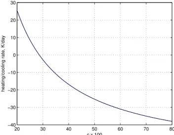
20 30 40 50 60 70 80 −40

−30 −20 −10 0 10 20 30

c x 100

heating/cooling rate, K/day

Fig. 6. Dependence of heating/cooling by eddy turbulence on the value ofc, using Eq. (4) forKec=3×106cm2/s andH=6 km.

As seen from Fig. 6, eddy turbulence can heat the mesopause

forc <0.286 and cool it forc >0.286. The range ofcvalues

can be estimated. The ratio of the turbulent energy dissipa-tion rate due to the acdissipa-tion of viscous and buoyancy forces to the transfer rate of kinetic energy from the mean motion to the fluctuating motion,Qeds=Ked(∂u/∂z)2, is determined

by the ratio of the Richardson number,Ri=ω_B2(∂u/∂z)2, to the turbulent Prandtl number,P=Ked/Kec. In the case

of mean motion,ccan be estimated as being equal toRi/P. For the mean wind sheer of 20 m/s/km and ω_B2 =(3/5)×

10−4s−2, theRivalues are within the range of 0.75–1.25 and thecvalue is about 1 forP≈1. Thecvalue decreases with increasingP and turbulent heating can dominate cooling. In any case, we can estimate the sensitivity of turbulent heat-ing/cooling to the influence of wind shear and gravity waves. Now we consider the heating/cooling caused by eddy tur-bulence in more detail. The height profile of the tem-perature given by the MSISE-90 model below the polar mesopause can be approximated by a linear dependence with the gradient ∂T /∂z=G= −5.4 K/km in summer and G= −3.2 K/km in winter solstice at latitudes 70◦S and 70◦N, respectively. In this case, the density height distribution is given by the formula

ρ=ρ0

_T

0

T0−Gz

1−mg/κG

, (6)

and the heating/cooling rate given by Eq. (1) can be written as

Qed=Kec

Cp

Cv

τd

_g

Cp

−G

_G−mg/κ

T0−Gz

+∂Kec

∂z

Cp

CV

τd

_g

Cp

−G

+Kec

τdg

Cvc(T0−Gz)

_g

Cp

−G

80 85 90 95 100 −50

−40 −30 −20 −10 0 10 20 30

height, km

heating rate, K/day

Fig. 7. The height profile heating/cooling rates calculated by Eq. (7) for summer conditions (zm=90 km, c=0.3, mesopause height = 90 km,G= −4 K/km below 90 km, andG=5 K/km above 90 km).

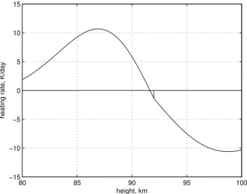
80 82 84 86 88 90

−25 −20 −15 −10 −5 0 5 10 15

height, km

heating rate, K/day

Fig. 8. The same as in Fig. 7 but below theKec peak and with c=0.8.

The first term on the right side of Eq. (7) is negative because mg/κis much larger thanG. The second term is positive be-low theKecpeak and is negative above theKec peak. The

eddy diffusion coefficient inferred by L¨ubken (1997) from measurements of the turbulent energy dissipation rate in the summer polar mesosphere can be approximated by the for-mulas suggested by Shimazaki (1971):

Kec=Kec0exp[S1(z−zm)]+

K_ecm−K_ec0exph−S2(z−zm)2

i

z≤zm (8)

Kec=Kecmexp

h

−S3(z−zm)2

i

z > zm (9)

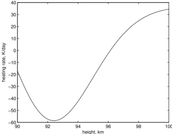
90 92 94 96 98 100

−60 −50 −40 −30 −20 −10 0 10 20 30 40

height, km

heating rate, K/day

Fig. 9. The same as in Fig. 8 but above theKedpeak and with c=0.8.

whereK_ecm=1.8×106cm2/s is the maximum of these coef-ficients,zm=90 km,S1=0.05 km−1,S2=0.04 km−2, and S3=0.05 km−2. The same approximation is used in the

[O] calculations. The height profiles of the heating/cooling rate calculated by Eq. (7) forc=0.3 and 0.8 are shown in Figs. 7, 8, and 9. Note that the summer polar mesopause is located at an altitude of 90 km, according to the MSISE-90 model. Thus, the cooling rates calculated with the eddy dif-fusion coefficient inferred from measurements are found to be−13.5 K/day and−41.5 K/day forc=0.3 andc=0.8, re-spectively, at the mesopause. The strong change in the cool-ing rate withcis explained by the strong increase in the dis-sipative term in Eq. (7) with thecvalue decrease.

Using the same approach, we have calculated the heat-ing/cooling rates in the polar winter mesosphere. The height profiles of these rates forc=0.3 andc=0.8 are shown in Figs. 10 and 11. Note that we increased the altitude of the

Kecpeak from 90 km (given by L¨ubken) to 92 km because,

according to the MSISE-90 model, the altitude of the tur-bopause inferred from the vertical profiles of theAr/N2ratio

is higher in winter than in summer. Comparing the cool-ing rates in the summer and winter mesopause, it is clear that the turbulent cooling rate in the winter mesosphere is much less than the cooling rate in the summer mesopause. This strong winter-summer asymmetry is well known (e.g., Becker, 2004).

As seen from the results discussed above, eddy turbulence cools the mesosphere at altitudes above and below theKec

peak for c >0.3, and the maximum of this cooling rate is

−30 K/day−50 K/day in summer and−10 K/day in winter. Note that the maximum adiabatic cooling rate calculated by the SOCRATES model in the polar summer mesopause is

80 85 90 95 100 −20

−15 −10 −5 0 5 10

height, km

heating rate, K/day

Fig. 10.The height profile of heating/cooling rates for winter condi-tions withc=0.8, a mesopause height of 100 km,G=3 K/km be-low 92 km, andG=2 K/km above 92 km. The vertical line shows theKedpeak location.

80 85 90 95 100

−15 −10 −5 0 5 10 15

height, km

heating rate, K/day

Fig. 11.The same as in Fig. 10 but withc=0.3.

adiabatic rate. The maximum of the turbulent heating rate does not exceed +10 K/day, which is smaller than for adia-batic heating. Our results differ from the results of Fritts and Luo (1995) mentioned above because their model gives aKec

peak at an altitude of 105 km. However, thisKecpeak

loca-tion contradicts the MSISE-90 model because the turbopause altitude calculated using theAr/N2 ratio is about 90 km in

the polar summer MLT. In addition, radar observations by Ecklund and Balsley (1981) show that echoes in the summer polar mesosphere are caused by turbulence below 98 km.

In the previous section, it was mentioned that the eddy diffusion coefficient should be increased by a factor of 2–3 if upward/downward motion occurs. In this case, the Prandtl number is larger than one and localized turbulent layers can take place.

4 Conclusion

Our results show that seasonal variations of the O den-sity and the altitude of the [O] peak, calculated with up-ward/downward motion corresponding to adiabatic cool-ing/heating, are opposite to the observed seasonal variations given by the MSISE-90 model. Eddy turbulence with coeffi-cients close to the values inferred from experimental data by L¨ubken (1997) can provide the observed seasonal variations of the O density and the altitude of the [O] peak. The heat-ing/cooling by this eddy turbulence is comparable to or larger than adiabatic heating/cooling in the upper mesosphere. The strong impact of upward/downward motion and eddy turbu-lence on the [O] height distributions requires self-consistent modeling of the O density and temperature because of the im-portant role of atomic oxygen in infrared cooling and chem-ical heating in the upper mesosphere. The eddy diffusion coefficients should be increased by a factor of 2–3 in order to obtain summer and winter [O] profiles close to the MSISE-90 data if upward/downward motion, corresponding to adiabatic cooling/heating, is taken into account.

Acknowledgements. Topical Editor C. Jacobi thanks E. Becker and

another anonymous referee for their help in evaluating this paper.

References

Akmaev, R. A.: On the energetics of mean-flow interactions with thermally dissipating gravity waves, J. Geophys. Res., 112, D11125, doi:10.1029/2006JD007908, 2007.

Becker, E.: Direct heating rates associated with gravity wave satu-ration, J. Atmos. Solar-Terr. Phys., 66(6–9), 683–696, 2004. Becker, E. and McLandress, C.: Consistent scale interaction of

gravity waves in the Doppler spread parameterization, J. Atmos. Sci., 66, 1434–1449, 2009.

Banks, P. M. and Kockarts, G.: Aeronomy, Academic Press, New York, 1973.

Berger, U. and von Zahn, U.: The two-level structure of the mesopause: A model study, J. Geophys. Res., 104, 22083– 22093, 1999.

Brasseur, G. P. and Solomon, S.: Aeronomy of the Middle Atmo-sphere, 2nd ed., 452 pp., D. Reidel Pub. Co., Norwell, Mass., 1986.

Brasseur, G., Smith, A. K., Khosravi, R., Huang, T., Walters, S., Chabrillat, S., and Kockarts, G.: Natural and human-induced per-turbations in the middle atmosphere: A short tutorial, in: Atmo-spheric Science Across the Stratopause, edited by: Siskind, D. E., Eckermann, S. D., and Summers, M. E., American Geophys-ical Union, Washington, D.C., 7–20, 2000.

Dunkerton, T. J.: On the mean meridional mass motions of the stratosphere and mesosphere, J. Atmos. Sci., 35, 2325–2333, 1978.

Ecklund, W. L. and Balsley, B. B.: Long-term observations of the arctic mesosphere with the MST radar at Poker Flat, Alaska, J. Geophys. Res., 86, 7775–7780, 1981.

Canadian Middle Atmosphere Model: Zonal-mean climatol-ogy and physical parameterization, J. Geophys. Res., 107(D10), 4087, doi:10.1029/2001JD000479, 2002.

Fritts, D. C. and Luo, Z.: Dynamical and radiative forcing of the summer mesopause circulation and thermal structure 1. Mean solstice conditions, J. Geophys. Res., 100, 3119–3128, 1995. Fukao, S., Yamanaka, M., Ao, N., Hocking, W., Sato, T.,

Ya-mamoto, M., Nakamura, T., Tsuda, T., and Kato, S.: Seasonal variability of vertical eddy diffusivity in the middle atmosphere 1. Three-year observations by the middle and upper atmosphere radar, J. Geophys. Res., 99(D9), 18973–18987, 1994.

Gardner, C. S. and Yang, W.: Measurements of the dynamical cool-ing associated with vertical transport of heat by dissipatcool-ing grav-ity waves in the mesopause region at the Starfire Optical Range, New Mexico, J. Geophys. Res., 103, 16909–16926, 1998. Hedin, A. E.: Extension of the MSIS thermospheric model into the

lower and middle atmosphere, J. Geophys. Res., 96, 1159–1172, 1991.

Hill, R. J., Gibson-Wilde, D. E., Werne, J. A., and Fritts, D. C.: Turbulence-induced fluctuations in ionization and application to PMSE, Earth Planets Space, 51, 499–513, 1999.

Hines, C. O.: Doppler-spread parameterization of gravity wave mo-mentum deposition in the middle atmosphere. Part 1: Basic for-mulation, J. Atmos. Solar-Terr. Phys., 59, 371–386, 1997. Hocking, W. K.: The dynamical parameters of turbulence theory as

they apply to middle atmospheric studies, Earth Planets Space, 51, 525–541, 1999.

Larsen, M. F.: Winds and shears in the mesosphere and lower thermosphere: Results from four decades of chemi-cal release wind measurements, J. Geophys. Res., 107, 1215, doi:10.1029/2001JA000218, 2002.

L¨ubken, F.-J.: Seasonal variations of turbulent energy dissipation rates at high altitudes as determined by in situ measurements of neutral density fluctuations, J. Geophys. Res., 102, 13441– 13456, 1997.

Medvedev, A. S. and Klaassen, G. P.: Thermal effect of saturating gravity waves in the atmosphere, J. Geophys. Res., 108, 4040, doi:10.1029/2002JD002504, 2003.

Shimazaki, T.: Effective eddy diffusion coefficient and atmospheric composition in the lower thermosphere, J. Atmos. Terr. Phys., 33, 1383–1401, 1971.

Smith, A. K.: Physics and chemistry of the mesopause region, J. Atmos. Solar-Terr. Phys., 66, 839–857, 2004.

Vlasov, M. N. and Davydov, V. E.: Theoretical description of the main neutral constituents in the earth’s upper atmosphere, J. At-mos. Terr. Phys., 44, 641–647, 1982.

Vlasov, M. N. and Davydov, V. E.: The effect of vertical transfer on the composition of the thermosphere during geomagnetic distur-bances, Kosmicheskie Issled, 21, 725–730, 1983.