www.ann-geophys.net/26/3225/2008/ © European Geosciences Union 2008
Annales
Geophysicae
Comparison of ECMWF analyses with GPS radio occultations from
CHAMP
T. Schmidt1, J. Wickert1, S. Heise1, F. Flechtner1, E. Fagiolini2, G. Schwarz2, L. Zenner3, and T. Gruber3
1Helmholtz Centre Potsdam, GFZ German Research Centre for Geosciences, Telegrafenberg A17, 14473 Potsdam, Germany 2Deutsches Zentrum f¨ur Luft- und Raumfahrt, M¨unchener Straße 20, 82234 Weßling, Germany
3Technische Universit¨at M¨unchen, Arcisstraße 21, 80333 M¨unchen, Germany
Received: 20 May 2008 – Revised: 23 July 2008 – Accepted: 27 August 2008 – Published: 21 October 2008
Abstract. A climatological validation of the 6-hourly op-erational ECMWF troposphere and lower stratosphere tem-peratures as well as geopotential heights between 1000 and 10 hPa is performed using the 2001–2007 (80 months from May 2001 to December 2007) CHAMP radio occultation data. Generally there is a good agreement between ECMWF and CHAMP temperatures averaged over 300–10 hPa for all years/seasons with global annual mean biases (standard devi-ations) less than 0.3 (1.7) K. Regional and temporal discrep-ancies occur within the polar vortex mainly on the South-ern Hemisphere and the tropical tropopause region. Global annual mean biases (standard deviations) of geopotential heights between 300 and 10 hPa are in the range of −30
up to +5 (30–50) geopotential meter. Larger deviations from the mean values are also observed in the tropics and polar zones. Both, the biases and standard deviations be-tween CHAMP and ECMWF temperatures and geopoten-tial heights differ significantly before and after February and December 2006, i.e. the dates when ECMWF increased the number of model levels from L60 to L91 (1 February 2006) and where ECMWF became one of the first weather cen-ters assimilating radio occultation data (since 12 December 2006), mainly from the COSMIC mission. At ECMWF the CHAMP data were only assimilated until 4 February 2007, e.g. both data sets are mostly independent from each other during the time period considered here.
Keywords. Meteorology and atmospheric dynamics
(Cli-matology; Middle atmosphere dynamics; Instruments and techniques)
Correspondence to:T. Schmidt ([email protected])
1 Introduction
The European Centre for Medium-Range Weather Forecasts (ECMWF) operational analyses from the Integrated Fore-casting System (ECMWF, 2007a) are widely used for several applications in atmospheric research. Additionally, the daily 6-hourly analyses are also applied in adjacent fields needing information about the global atmospheric state on different time scales.
For example, a remaining problem for the GRACE (Grav-ity Recovery And Climate Experiment) grav(Grav-ity field anal-ysis is the de-aliasing of short-term non-tidal atmospheric and oceanic mass variations (Tapley et al., 2004; Flechtner et al., 2006). For computation of the atmospheric contribution and for forcing of the used ocean model various parameters from an atmospheric weather model, such as surface pres-sure, geopotential height (GPH), and temperature and humid-ity at different vertical levels, are applied. These atmospheric parameters are assumed to be error free. Any departure from this assumption leads to aliasing and misinterpretation of the resulting gravity field. Therefore, for all atmospheric param-eters realistic error characterizations should be established.
The current atmospheric model for the GRACE gravity field analysis is the ECMWF operational model. One way to develop error measures is to compare the ECMWF model with other data bases, e.g. from the National Center for En-vironmental Prediction (NCEP) or with independent global atmospheric data sets.
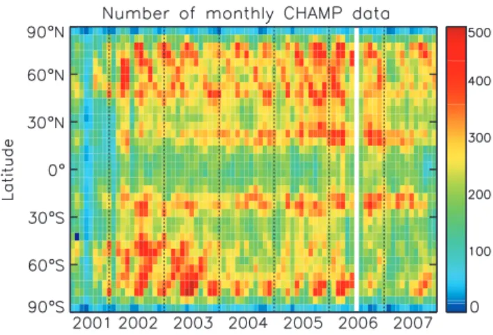
Fig. 1.Zonal monthly mean number of GPS RO CHAMP data from May 2001–December 2007.
resolution (Kursinski et al., 1997; Rocken et al., 1997; Mel-bourne et al., 1994). Mean biases and standard deviations (stddev) of the compared parameters will be shown and dis-cussed.
Careful attention is given to the fact that the ECMWF as-similation scheme has experienced two important changes during the time period considered here: First, the number of vertical model levels was increased from L60 to L91 in February 2006 (ECMWF, 2006). Second, ECMWF became one of the first weather centers (since 12 December 2006) assimilating GPS RO data (Healy et al., 2007; Healy, 2007; ECMWF, 2007b; Bormann and Healy, 2005), mainly from the US-Taiwanese COSMIC (Constellation Observing Sys-tem for Meteorology, Ionosphere, and Climate) mission (An-thes et al., 2008). CHAMP data were assimilated at ECMWF only until 4 February 2007 (S. Healy, ECMWF, personal communication, 2008), i.e. with the exception of the time in-terval between 12 December 2006 and 4 February 2007 (55 days) the ECMWF and CHAMP data sets used here can be considered independent from each other. Changes in mean biases and stddev between the pre- and post-assimilation pe-riods will be pointed out.
Nevertheless, the most important parameter for GRACE de-aliasing is the surface pressure, which does not change significantly by these changes in the assimilation scheme.
In the past, several comparison studies between GPS RO data and radiosondes as well as cross-validations with other satellite sensors have already been performed (e.g. Steiner et al., 2007; Gobiet et al., 2007; Wickert, 2004a; Wang et al., 2004; Hajj et al., 2004). Special comparisons of tropopause parameters between CHAMP and ECMWF can be found in, e.g. Borsche et al. (2007) and Schmidt et al. (2006, 2005a, 2004).
For a climatological validation of stratospheric tempera-tures between ECMWF and CHAMP for 2001–2004, see Gobiet et al. (2005). This is the most comprehensive
val-In Sect. 3 we discuss the results according to the complete time interval considered here, the latitude-time section of mean biases and stddevs, and seasonal variations. At the end a summary and conclusions follow.
2 Data processing and validation methodology
2.1 CHAMP data processing
2.1.1 Deriving atmospheric parameters
A detailed general description to derive vertical atmospheric profiles from RO measurements is presented by Melbourne et al. (1994) or Kursinski et al. (1997); specifications for the CHAMP RO data can be found in Wickert et al. (2005) or Hajj et al. (2004). Here, we give a brief summary: The Black-Jack GPS receiver onboard CHAMP records phase and amplitude variations with high temporal resolution (50 Hz) during an occultation event. By using high precision orbit information from CHAMP and the occulting GPS satel-lites (K¨onig et al., 2005) the atmospheric excess phase can be extracted which is related to a bending angle profile. Assum-ing spherical symmetry the bendAssum-ing angles can be related to the refractive indexn. Finally, the atmospheric refractivityN
is given by (Smith and Weintraub, 1953):
N =(n−1)·106=77.6p
T +3.73·10
5ew
T2 (1) (withp: total air pressure,T: air temperature, andew: water vapor pressure). N is the basic meteorological observable determined by the GPS RO technique.
To convert the refractivity profiles into pressure and tem-perature profiles the assumption of dry air has to be made because of the ambiguity between the dry and wet part in the resulting refractivity profile (Eq. 1). Further on, by apply-ing the hydrostatic equation pressure and temperature pro-files can be calculated. In the current retrieval version 005 (Wickert et al., 2004b) ECMWF pressure at 43 km is used for the initialization of the pressure profile. This is one atmo-spheric scale height above the upper level for which profile data are provided (35 km).
(a) (b)
(c) (d)
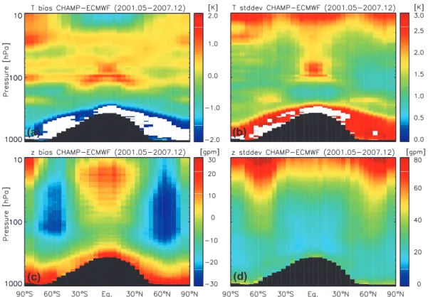
Fig. 2. Zonal mean temperature bias(a), temperature stddev(b), GPH bias(c)and GPH stddev between CHAMP and ECMWF for the pressure (altitude) range 1000–10 hPa and the time interval May 2001–December 2007. The meridional resolution is 5◦between 77.5◦N– 77.5◦S and 10◦for 85◦N and 85◦S. The vertical pressure resolution corresponds to an altitude resolution of about 200–300 m. The black areas denote regions with temperatures above 250 K. In the white areas the bias is less than−2 K (a) and the stddev is larger than 3 K (b).
this criterion, i.e. we compared CHAMP and ECMWF tem-peratures as well as GPHs only if the temperature of both data sets was below 250 K.
2.1.2 Vertical resolution
The vertical resolution of an occultation measurement is de-termined by the contribution of individual atmospheric layers to net bending along the ray path. As discussed in Kursinski et al. (1997) by using the geometrical optics approach the vertical resolution is limited by the diameter of the first Fres-nel zonezF. For the CHAMP orbit geometry zF is about
1.4 km in the stratosphere (about 270 km horizontal resolu-tion). Because of the exponential increase of the refractiv-ity towards the Earth’s surfacezF decreases to about 0.5 km
(horizontal resolution about 80 km).
Considering diffraction effects and applying wave optical methods for the data analysis as, e.g. the Full Spectrum Inver-sion (FSI) method (Jensen et al., 2003) the vertical resolution can be improved significantly (to about 50 m).
In our current software version (005) we have imple-mented both, the geometrical optics approach for heights above 15 km and the FSI method for heights below 10 km. In the transition zone from 10–15 km a combination of both
is used. This results in a physical vertical resolution of about 1 km above 15 km altitude and a vertical resolution less than 1 km below. For data provision all data were interpolated be-tween the lowest level and 35 km with a vertical step width of 200 m.
2.2 The data base
CHAMP delivers continuously between 150–200 temper-ature profiles daily (Wickert et al., 2005; Schmidt et al., 2005b) since May 2001. Thus, the CHAMP mission gen-erates the first long-term GPS RO data set. Figure 1 shows the zonal monthly mean number of CHAMP data for the time interval May 2001–December 2007 (more than 439 000 tem-perature profiles).
In the monthly time series one month was rejected com-pletely if only data from less than 50% of the days per month were available. This exclusion criteria was fulfilled for July 2006 only.
2.3 Validation methodology
(b)
(a)
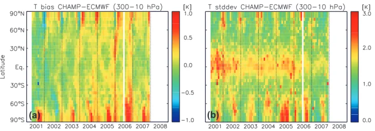
Fig. 3.Zonal monthly mean temperature bias(a)and stddev(b)between CHAMP and ECMWF averaged over the pressure (altitude) range 300–10 hPa. The meridional resolution is 5◦between 77.5◦N–77.5◦S and 10◦for 85◦N and 85◦S (34 latitude bands).
Fig. 4. Global, northern hemispheric and southern hemispheric monthly mean temperature bias and stddev between CHAMP and ECMWF for the pressure (altitude) range 300–10 hPa. The left side of the shaded area denote the month when the ECMWF model lev-els have increased from 60 to 91 (February 2006), the right side of the shaded area corresponds to the beginning of the assimilation of GPS RO data at ECMWF (December 2006). The yearly horizontal lines denote the annual mean of the bias and stddev, respectively.
the 6-hourly operational ECMWF data sets to the time of the occultation event, whereas the ECMWF temperature fields are extracted on all model levels (T511/L60 until 1 Febru-ary 2006 and T799/L91 after) with a reduced horizontal resolution of about 0.56◦ in latitude and longitude (T319).
All changes in the ECMWF analysis and forecasting system since 1985 are available at www.ecmwf.int/products/data/ operational system/evolution.
Because the CHAMP and ECMWF profiles are not avail-able at the same altitude or pressure levels, the comparison
of temperature and GPH data were performed on 153 con-stant pressure levels beween 1000 and 10 hPa, representing approximately a vertical resolution of 200–300 m. For this reason each individual CHAMP and ECMWF profile was in-terpolated to these pressure levels and temperature/GPH dif-ferences were determined if both, the CHAMP and ECMWF temperature was below 250 K (see above for this criterion).
The determination of systematic biases and stddevs re-quires the analysis of differences between CHAMP and ECMWF profiles. It has to be noted, however, that both types of profiles are characterized by slightly different ver-tical resolutions. Following good practice, we should adapt the resolutions prior to taking the differences. This, however, requires the availability of correct averaging kernels as dis-cussed by Rodgers (2000). As no validated averaging kernels of the CHAMP retrieval were available to us, we had to limit ourselves to a direct differencing.
For statistical evaluation monthly zonal biases/stddevs are calculated at the selected pressure levels. The zonal bins were divided into 5◦ latitude bands centered at 77.5◦N, 72.5◦N, 67.5◦N, ..., 67.5◦S, 72.5◦S, 77.5◦S (32 latitude bands). Due to the poorer monthly data coverage at the poles (Fig. 1) two 10◦ latitude bands centered at 85◦N and 85◦S
were used leading to a total of 34 latitudes bands.
3 Results
3.1 The complete data set analysis 3.1.1 Temperature
(b)
(a)
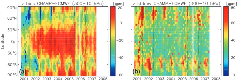
Fig. 5.Same as Fig. 3, but for the GPH.
observed: The overall temperature bias (Fig. 2a) varies gen-erally between±1.5 K in the extra-tropics above 300 hPa. In
the tropics (30◦N–30◦S) the±1.5 K bias is reached above
the 200 hPa level.
The negative temperature bias exceeding−2 K in the tro-posphere (white area in Fig. 2a) can be clearly addressed to the non-consideration of water vapor in the temperature re-trieval (Eq. 1). Apparently, the “below 250 K temperature criterion” where water vapor should be negligible (Kursinski et al., 1997) seems to be questionable.
The positive temperature bias (>1 K) in the tropical tropopause and the adjacent regions above (120–60 hPa) was already discussed in Gobiet et al. (2005) or Borsche et al. (2007) and is probably related to the lower vertical resolution of the ECMWF model in general. As a consequence, the pos-sibility to dissolve gravity waves in the lower tropical strato-sphere is weak compared with the CHAMP data set leading to enhanced stddevs (Fig. 2b). The stratospheric temperature bias structure in the polar regions (“stratospheric ringing”, weakly implied in the overall plot) was also a topic in Gob-iet et al. (2005) and will be discussed here later mainly with respect to the changes in the ECMWF assimilation scheme.
Generally, the temperature bias is larger on the Southern Hemisphere (SH) than in the Northern Hemisphere (NH) re-sulting from the sparse coverage of the SH with radiosonde observations. The appropriate mean stddev (Fig. 2b) for the time interval considered here is less than 3 K in the altitude ranges with temperature biases between±1.5 K. Largest
std-dev values are observed above 20 hPa. 3.1.2 Geopotential heights
The overall bias and stddev of the GPHs between CHAMP and ECMWF are shown in Fig. 2c, d. Zonal mean values ranging between±30 geopotential meter (gpm) for the bias
Fig. 6.Same as Fig. 4, but for the GPH.
and up to 80 gpm for the stddev for regions with temperatures less than 250 K.
In the tropics and subtropics (40◦N–40◦S) on both hemi-spheres the mean GPH bias between 250–10 hPa is about
±15 gpm with a mean stddev less than 50 gpm (for the com-plete time interval 2001–2007).
In the mid-latitudes and polar zones both the bias and std-dev increase. The pronounced lower stratospheric negative GPH bias of up to−30 gpm centered at 60◦on both hemi-spheres is remarkable. The SH minimum coincides with the climatological location of the relatively stable SH polar vortex, whereas the NH minimum is broader reflecting the much larger lower stratospheric synoptic variability between 50◦N–80◦N.
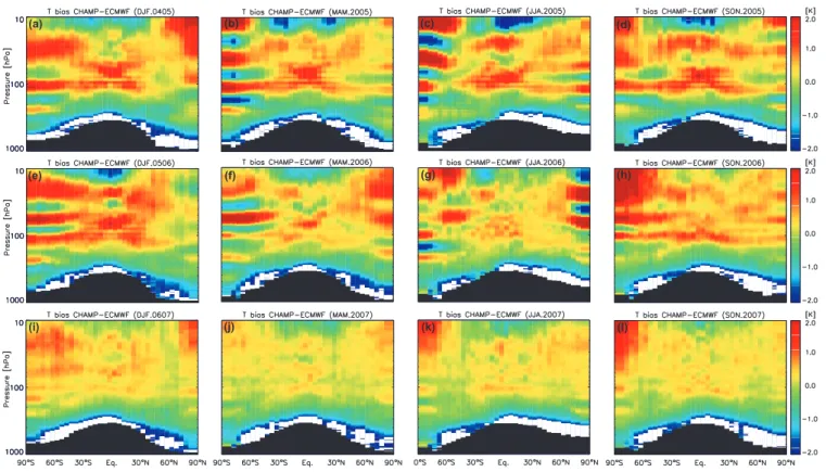
(i) (j) (k) (l)
Fig. 7. Zonal mean temperature bias between CHAMP and ECMWF for the pressure (altitude) range 1000–10 hPa for different seasons (DJF.0405–SON2007). The meridional resolution is 5◦between 77.5◦N–77.5◦S and 10◦for 85◦N and 85◦S. The vertical pressure resolu-tion corresponds to an altitude resoluresolu-tion of about 200–300 m. The black areas denote regions with temperatures above 250 K. In the white areas the bias is less than−2 K.
spring whereas the positive tropical bias between 50–10 hPa is significantly reduced after the increase of the ECMWF model levels in February 2006 (see Fig. 9).
3.2 Time-latitude variations
The previous section gave an overview about the mean temperature and GPH bias as well as the stddev between CHAMP and ECMWF for the complete time period con-sidered here and could be interpreted as the mean state. In the following we go more in detail with respect to the time evolution of the temperature and GPH differences between CHAMP and ECMWF.
The possible quantities describing the goodness of the de-viations between CHAMP and ECMWF here are mean tem-peratures and GPH biases/stddevs between 300–10 hPa. As shown in Fig. 2 the influence of water vapor can be neglected in that region even in the tropics.
3.2.1 Temperature
Figure 3 shows the monthly evolution of the zonal tempera-ture bias and stddev. It can be seen that the mean bias has a maximum in the polar zones during winter/spring. The
extra-tropical stddev follows the bias pattern whereas the extra-tropical temperature stddev is also enhanced reaching values compa-rable to those in the polar regions.
We do not interpret all variations of the bias and stddev with respect to the changes in ECMWF assimilation scheme, but focus here on February 2006 (L60 to L91) and December 2006 (assimilation of GPS RO data).
It is already visible in Fig. 3a that apart from annual cy-cles the mean bias between 300–10 hPa increases at nearly all latitudes between 2001 and 2006. In 2007 (after assimila-tion of RO data) the temperature bias seems to be decreased globally.
To revise this trend we defined global monthly mean tem-perature biases/stddevs by cosine-weighted means of the sin-gle zonal means (Fig. 4). The positive temperature bias trend until 2006 is notable. The improvement of the vertical model resolution seems to have no impact on the temperature bias, but the assimilation of RO data in late 2006. The annual tem-perature bias in 2007 has nearly vanished.
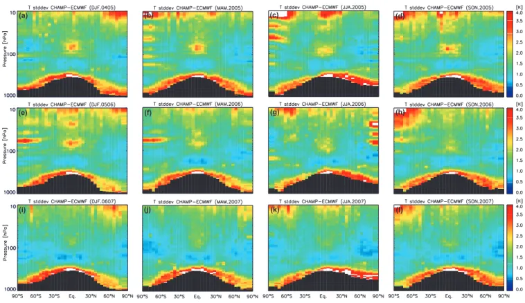
(a) (b) (c) (d)
(e) (f) (g) (h)
(i) (j) (k) (l)
Fig. 8.Same as Fig. 7, but for the stddev. In the white areas the stddev is larger than 4 K.
The improvements in both, the temperature bias and std-dev suggest the assumption that the new RO data have signed a considerable weight between 300–10 hPa in the as-similation scheme.
A comparison of the NH and SH temperature biass/stddevs show differences not exceeding 0.2 K with slightly higher SH biases indicating the better spatial coverage of the NH with radiosondes.
3.2.2 Geopotential heights
The latitude-time section of the mean GPH bias and stddev between 300–10 hPa is presented in Fig. 5. Values up to 20 gpm are observed in the tropics from 2002–2005. During the polar vortex season on the SH similar values are reached. In the mid-latitudes on both hemispheres negative GPH bi-ases are present with values up to−60 gpm in 2001 and 2002.
The corresponding stddev is enhanced in the mid-latitudes and polar regions on both hemispheres with maximum values of 80 gpm in 2001/2002 (Fig. 5b).
Figure 6 shows the temporal evolution of the global mean GPH bias and stddev between 300 hPa and 10 hPa. There is a similar positive GPH bias trend between 2001 and 2004 as already seen in the global temperature bias (Fig. 4). Dur-ing the same time period a decreased annual GPH stddev is observed from about 45 gpm down to 35 gpm.
In contrast to the temperature bias, the GPH bias in 2006 and 2007 is degraded after the ECMWF level number in-crease in February 2006 compared with the three years be-fore. From 2003–2005 the bias had nearly vanished, whereas 2006 and 2007 a slightly negative annual mean bias of about
−10 gpm is observed. The largest difference between the
mean annual temperature and GPH bias is that the latter is not affected by the assimilation of RO data.
The annual mean stddev is also not affected by the two changes in the assimilation scheme mainly considered here. The values are nearly constant since 2003 (35 gpm).
Considering differences between the hemispheres one can see that there is a slightly larger bias on the SH. The GPH stddev exhibits an annual cycle with a maximum in the ap-propriate winter season and a minimum during summer. The amplitude reaches nearly the same magnitude on both hemi-spheres during a year.
3.3 Seasonal variations
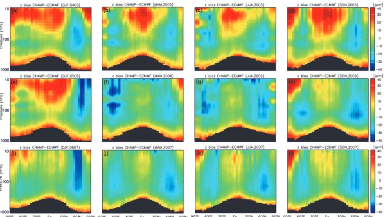
(i) (j) (k) (l)
Fig. 9.Zonal mean GPH bias between CHAMP and ECMWF for the pressure (altitude) range 1000–10 hPa for different seasons (DJF.0405– SON.2007). The meridional resolution is 5◦between 77.5◦N–77.5◦S and 10◦for 85◦N and 85◦S. The vertical pressure resolution corre-sponds to an altitude resolution of about 200–300 m. The black areas denote regions with temperatures above 250 K.
The seasons were classified as follows: December– February (DJF), March–May (MAM), June–August (JJA), and September–November (SON).
Figure 7 shows the CHAMP–ECMWF temperature bias between the seasons DJF 2004/2005 and SON 2007. Most of the bias structure observed for the complete time interval can be also found here (Fig. 2a).
The most remarkable feature in the polar lower strato-sphere first described by Bormann and Healy (2005) and Go-biet et al. (2005) is the so-called “stratospheric ringing” pat-tern. This temperature bias structure is more or less observed in the SH polar stratosphere as well as in the northern part (Fig. 7a–h). Gobiet et al. (2005) discussed this bias in con-nection with the assimilation of AMSU-A radiances whose temperature weighting functions for different channels are close to the bias wave pattern. The final conclusion of Go-biet et al. (2005) is that the temperature bias can be clearly attributed to the ECMWF analysis.
Due to the inclusion of the GPS RO data in the ECMWF operational model the ’stratospheric ringing’ structure disap-peared (Fig. 7i–l). As already discussed in Sect. 3.2.1 (Fig. 4) there is nearly no temperature bias between CHAMP and ECMWF between 300–10 hPa after assimilation of the RO data (Fig. 7i–l). From this we conclude that the RO data gain high priority in the ECMWF assimilation scheme.
For completion, Fig. 8 presents the seasonal temperature stddev with some of the same features as observed in the temperature bias. During the time before December 2006 also a ringing structure of the stddev can be found which has vanished afterwards.
The seasonal variation of the GPH bias between 2005– 2007 is shown in Fig. 9. As discussed above one can clearly see the significant reduction of the positive tropical lower stratospheric bias after increase of the ECMWF model lev-els from L60 to L91 whereas the assimilation of RO data has nearly no effect. The negative GPH bias in the mid-latitudes and sub-polar regions is present all the time, but slightly re-duced after DJF 2006/2007 (Fig. 9j–l).
4 Summary
In this study we have compared ECMWF temperature and GPHs between 1000–10 hPa for the time interval May 2001 and December 2007.
than 0.1 K in 2007 after the assimilation of GPS RO data at ECMWF. The according temperature stddev in 2007 (1.5 K) was also reduced compared with the pre-assimilation period (between 1.6–1.7 K). The ’stratospheric ringing’ observed in the temperature bias/stddev of the polar lower strato-sphere disappeared after the assimilation of GPS RO data at ECMWF in December 2006.
Global annual mean biases (stddevs) of GPHs between 300–10 hPa are in the range of −30 and +5 (30–50) gpm.
The CHAMP–ECMWF GPH bias is more influenced by the increase of the ECMWF model levels from L60 to L91 than the assimilation of RO data.
Acknowledgements. The authors would like to thank all other mem-bers of the CHAMP team for their contributions to this study and the ECMWF for supplying the operational weather analyses. This work is funded through the research project ’IDEAL-GRACE’ within the DFG priority program 1257 “Mass Transports and Mass Distribu-tion in the Earth System”.
Topical Editor F. D’Andrea thanks two anonymous referees for their help in evaluating this paper.
References
Anthes, R. A., Bernhardt, P. A., Chen, Y., et al.: The COSMIC/FORMOSAT-3 mission: Early results, B. Am. Meteo-rol. Soc., 89, 1–21, 2008.
Bormann, N. and Healy, S. B.: New observations in the ECMWF assimilation system: Satellite limb measurements, ECMWF Newsletter, 105, 13–17, 2005.
Borsche, M., Kirchengast, G., and Foelsche, U.: Tropi-cal tropopause climatology as observed with radio occul-tation measurements from CHAMP compared to ECMWF and NCEP analyses, Geophys. Res. Lett., 34, L03702, doi:10.1029/2006GL027918, 2007.
European Centre for Medium-Range Weather Forecasts (ECMWF): IFS Documentation – Cy31r1 Part II–IV, Reading, UK, 2007a. European Centre for Medium-Range Weather Forecasts (ECMWF):
Changes to the operational forecasting system, ECMWF Newsletter, 110, p. 2, 2007b.
European Centre for Medium-Range Weather Forecasts (ECMWF): Changes to the operational forecasting system, ECMWF Newsletter, 106, p. 2, 2006.
Flechtner, F., Schmidt, R., and Meyer, U.: De-aliasing of short-term atmospheric and oceanic mass variations for GRACE, in: Observation of the Earth System from Space, edited by: Flury, J., Rummel, R., Reigber, Ch., Rothacher, M., Boedecker, G., and Schreiber, U., Springer, 83–97, 2006.
Gobiet, A., Kirchengast, G., Manney, G. L., Borsche, M., Retscher, C., and Stiller, G.: Retrieval of temperature profiles from CHAMP for climate monitoring: intercomparison with Envisat MIPAS and GOMOS and different atmospheric analyses, Atmos. Chem. Phys., 7, 3519–3536, 2007,
http://www.atmos-chem-phys.net/7/3519/2007/.
Gobiet, A., Foelsche, U., Steiner, A. K., Borsche, M., Kirchengast, G., and Wickert, J.: Climatological validation of stratospheric temperatures in ECMWF operational analyses with CHAMP
radio occultation data, Geophys. Res. Lett., 32(12), L12806, doi:10.1029/2005GL022617, 2005.
Hajj, G. A., Ao, C. O., Iijima, B. A., Kuang, D., Kursinski, E. R., Mannucci, A. J., Meehan, T. K., Romans, L. J., de la Torre Juarez, M., and Yunck, T. P.: CHAMP and SAC-C atmospheric occultation results and intercomparisons, J. Geophys. Res., 109, D06109, doi:10.1029/2003JD003909, 2004.
Healy, S. B., Wickert, J., Michalak, G., Schmidt, T., and Beyerle, G.: Combined forecast impact of GRACE-A and CHAMP GPS radio occultation bending angle profiles, Atmos. Sci. Lett., 8, 43– 50, 2007.
Healy, S. B.: Operational assimilation of GPS radio occultation measurements at ECMWF, ECMWF Newsletter, 111, 6–11, 2007.
Jensen, A. S., Lohmann, M., Benzon, H. H., and Nielsen, A.: Full Spectrum inversion of radio occultation signals, Radio Sci., 38(3), 1040, doi:10.1029/2002RS002763, 2003.
K¨onig, R., Michalak, G., Neumayer, K. H., Schmidt, R., Zhu, S. Y., Meixner, H., and Reigber, C.: Recent developments in CHAMP orbit determination at GFZ, in: Earth Observation with CHAMP, edited by: Reigber, C., L¨uhr, H., Schwintzer, P., and Wickert, J., Springer, Berlin, ISBN 3-540-22804-7, 65–70, 2005.
Kursinski, E. R., Hajj, G. A., Hardy, K. R., Schofield, J. T., and Lin-field, R.: Observing Earth’s atmosphere with radio occultation measurements using the Global Positioning System, J. Geophys. Res., 102, 23 429–23 465, 1997.
Leroy, S. S.: Measurement of geopotential heights by GPS radio occultation, J. Geophys. Res., 102, 6971–6986, 1997.
Melbourne, W. G., Davis, E. S., Hajj, G. A., Hardy, K. R., Kursin-ski, E. R., Meehan, T. K., and Young, L. E.: The application of spaceborne GPS to atmospheric limb sounding and global change monitoring, JPL Publication, 94–18, Jet Propulsion Lab-oratory, Pasadena, California, 1994.
Rocken, C., Anthes, R. A., Exner, M., Hunt, D., Sokolovskiy, S., Ware, R., Gorbunov, M., Schreiner, W., Feng, D., Herman, B., Kuo, Y. H., and Zou, X.: Analysis and validation of GPS/MET data in the neutral atmosphere, J. Geophys. Res., 102(D25), 29 849–29 866, 1997.
Rodgers, C. D.: Inverse Methods for Atmospheric Sounding, The-ory and Practice, World Scientific, Singapore, 2000.
Schmidt, T., Beyerle, G., Heise, S., Wickert, J., and Rothacher, M.: A climatology of multiple tropopauses derived from GPS radio occultations with CHAMP and SAC-C, Geophys. Res. Lett., 33, L04808, doi:10.1029/2005GL024600, 2006.
Schmidt, T., Heise, S., Wickert, J., Beyerle, G., and Reigber, C.: GPS radio occultation with CHAMP and SAC-C: global moni-toring of thermal tropopause parameters, Atmos. Chem. Phys., 5, 1473–1488, 2005a,
http://www.atmos-chem-phys.net/5/1473/2005/.
Schmidt, T., Wickert, J., Beyerle, G., K¨onig, R., Galas, R., and Reigber, C.: The CHAMP atmospheric processing system for radio occultation measurements, in: Earth Observation with CHAMP, edited by: Reigber, C., L¨uhr, H., Schwintzer, P., and Wickert, J., Springer, Berlin, ISBN 3-540-22804-7, 597–602, 2005b.
the Earth system, Science, 305, 503–505, 2004.
Wang, D. Y., Stiller, G. P., von Clarmann, T., et al.: Cross-validation of MIPAS/ENVISAT and GPS-RO/CHAMP temperature profiles, J. Geophys. Res., 109, D19311, doi:10.1029/2004JD004963, 2004.
Wickert, J., Beyerle, G., K¨onig, R., Heise, S., Grunwaldt, L., Michalak, G., Reigber, C., and Schmidt, T.: GPS radio occulta-tion with CHAMP and GRACE: A first look at a new and promis-ing satellite configuration for global atmospheric soundpromis-ing, Ann. Geophys., 23, 653–658, 2005,
http://www.ann-geophys.net/23/653/2005/.