www.atmos-chem-phys.net/13/7225/2013/ doi:10.5194/acp-13-7225-2013
© Author(s) 2013. CC Attribution 3.0 License.
Atmospheric
Chemistry
and Physics
Geoscientiic
Geoscientiic
Geoscientiic
Geoscientiic
Diagnosing the transition layer at extratropical latitudes using MLS
O
3
and MOPITT CO analyses
J. Barr´e1,*, L. El Amraoui1, P. Ricaud1, W. A. Lahoz1,3, J.-L. Atti´e1,2, V.-H. Peuch4, B. Josse1, and V. Mar´ecal1 1CNRM-GAME, M´et´eo-France and CNRS URA 1357, Toulouse, France
2Laboratoire d’A´erologie, Universit´e de Toulouse, CNRS/INSU, Toulouse, France 3Norsk Institutt for Luftforskning, 2027 Kjeller, Norway
4European Centre for Medium-Range Weather Forecasts, Shinfield Park, Reading, UK *now at: National Center for Atmospheric Research, Boulder, Colorado, USA
Correspondence to:J. Barr´e ([email protected])
Received: 28 June 2012 – Published in Atmos. Chem. Phys. Discuss.: 28 August 2012 Revised: 10 June 2013 – Accepted: 27 June 2013 – Published: 30 July 2013
Abstract.The behavior of the extratropical transition layer (ExTL) is investigated using a chemistry transport model (CTM) and analyses derived from assimilation of MLS (Mi-crowave Limb Sounder) O3and MOPITT (Measurements Of Pollution In The Troposphere) CO data. We firstly focus on a stratosphere–troposphere exchange (STE) case study that occurred on 15 August 2007 over the British Isles (50◦
N, 10◦
W). We evaluate the effect of data assimilation on the O3–CO correlations. It is shown that data assimilation dis-rupts the relationship in the transition region. When MLS O3 is assimilated, CO and O3values are not consistent between each other, leading to unphysical correlations at the STE lo-cation. When MLS O3 and MOPITT CO assimilated fields are taken into account in the diagnostics the relationship hap-pens to be more physical. We then use O3–CO correlations to quantify the effect of data assimilation on the height and depth of the ExTL. When the free-model run O3 and CO fields are used in the diagnostics, the ExTL distribution is found 1.1 km above the thermal tropopause and is 2.6 km wide (2σ). MOPITT CO analyses only slightly sharpen (by
−0.02 km) and lower (by −0.2 km) the ExTL distribution. MLS O3analyses provide an expansion (by +0.9 km) of the ExTL distribution, suggesting a more intense O3 mixing. However, the MLS O3analyses ExTL distribution shows a maximum close to the thermal tropopause and a mean lo-cation closer to the thermal tropopause (+0.45 km). When MLS O3 and MOPITT CO analyses are used together, the ExTL shows a mean location that is the closest to the ther-mal tropopause (+0.16 km). We also extend the study at the
global scale on 15 August 2007 and for the month of August 2007. MOPITT CO analyses still show a narrower chemi-cal transition between stratosphere and troposphere than the free-model run. MLS O3 analyses move the ExTL toward the troposphere and broaden it. When MLS O3analyses and MOPITT CO analyses are used together, the ExTL matches the thermal tropopause poleward of 50◦
.
1 Introduction
the extratropical dynamical tropopause. The World Meteoro-logical Organization (2003) defined the ExTL as a transition layer with chemical characteristics intermediate between the upper troposphere and the lower stratosphere maintained by exchanges across the tropopause.
Diagnostics using tracer–tracer correlation can locate the ExTL in an empirical way. Fischer et al. (2000), Hoor et al. (2002) and Pan et al. (2004) used aircraft in situ measure-ments to provide an analysis of trace gas (H2O, CO, CO2, N2O, NOyand O3) correlations in the LMS. Trace gas cor-relations have been shown to be an effective method to diag-nose stratosphere–troposphere exchange (STE) and mixing processes in the LMS. Tracer–tracer correlation methods in the LMS are introduced by Fischer et al. (2000). A following study, Hoor et al. (2002), attempted to diagnose the seasonal variation of the tracer–tracer relationship in the LMS. These two studies have concluded that a transition layer is formed in the LMS as a result of troposphere-to-stratosphere transport. Pan et al. (2004) introduced the use of tropopause-relative coordinates in addition of the tracer–tracer correlation meth-ods, and Pan et al. (2007) proposed a set of three diagnostics to evaluate the representation of chemical transport processes in the extratropical tropopause.
This study uses the diagnostics proposed by Pan et al. (2007) that define a statistical way to characterize the location and the thickness of the mixing layer using tracer–tracer relationships. Diagnosing ExTL height and thickness from tracer–tracer relationships is empirical but remains a powerful tool for characterizing the extratropical UTLS region. These types of diagnostics rely on a statistical characterization of the transition layer instead of attempting to identify the tropopause as a single point. Results from these diagnostics therefore provide new perspectives on the transition from stratosphere to troposphere. Hegglin et al. (2009) showed that these diagnostics can be applied to satellite measurements of O3, CO and H2O to characterize the ExTL seasonal and latitudinal variations in height and depth at the global scale. A multi-model assessment showed that models with coarse vertical resolution are unable to represent faithfully the ExTL at extratropical latitudes (Hegglin et al., 2010). Due to their coarse resolution, models overestimate the spread and the location in height of the ExTL.
Data assimilation, which combines observational infor-mation and a priori inforinfor-mation from a model in an ob-jective way (Kalnay, 2003), has the capability to com-bine satellite trace gas measurements and chemistry trans-port models. Data assimilation studies that focused on UTLS chemical fields started with Cathala et al. (2003), who assimilated subsonic flight-level observations of ozone. Later, Semane et al. (2007) assimilated O3data from a limb sounder (Michelson Interferometer for Passive Atmospheric Sounding) to diagnose a case study of STE over arctic re-gions. It has been shown that assimilation of stratospheric ozone data from a limb sounder improves the spatial
struc-ture of the ozone fields in the UTLS. Jackson (2007) and Stajner et al. (2008) have assimilated MLS (Microwave Limb Sounder) O3data and shown the added value of data assimilation on UTLS ozone fields in the tropics and in the extratropics. Wargan et al. (2010) use the Ozone Monitoring Instrument and MLS O3 in a data assimilation experiment to discuss the improvements of data assimilation in the spa-tial ozone structure in the UTLS and the related limitations due to the model resolution. Barr´e et al. (2012) have assim-ilated MLS O3 at low and high horizontal resolution, and show the impact of data assimilation and resolution on the UTLS spatial structure and on the tropospheric ozone fields. Barret et al. (2008) assimilated MLS CO data to investigate the transport pathway of CO in the African upper troposphere during the monsoon season. Finally, El Amraoui et al. (2010) have used MLS O3and MOPITT (Measurement Of Pollution In The Troposphere) CO to diagnose a STE event. This last study showed that assimilated MOPITT CO allows for a bet-ter qualitative description of the stratospheric intrusion event. To constrain the model used in this study, we assimilate O3 stratospheric profiles from Aura/MLS and Terra/MOPITT CO tropospheric profiles into the MOCAGE (Mod`ele de Chimie Atmospherique `a Grande Echelle) chemical trans-port model (CTM). Data assimilation has the capability to overcome possible deficiencies of the MOCAGE model in the UTLS (see, e.g., Semane et al., 2007; Barret et al., 2008; El Amraoui et al., 2010; Barr´e et al., 2012). The aim of this study is to quantify the impact of the assimilation of O3and CO data on the UTLS at extratropical latitudes. We use the same case study as presented by El Amraoui et al. (2010) that considers a deep stratospheric intrusion on 15 August 2007 over the British Isles (50◦N, 10◦W). In this previous study,
detailed validation demonstrated the capability of CO and O3 analyses to better represent the STE. The set of diagnostics proposed by Pan et al. (2007) are used here to quantify the capability of CO and O3analyses to represent the STE event. We also propose to extend the set of diagnostics from re-gional to global scales in the extratropics for the month of August 2007. This allows for us to quantify the capability of MOPITT CO and MLS O3 assimilated fields to better esti-mate the chemical ExTL behavior, from a single STE event at the regional scale to an average state of the atmosphere at the global scale. To our knowledge, this is the first time that these diagnostics have been used on chemical analyses from different types of satellite measurements (nadir and limb).
2 Methodology
2.1 CTM and data assimilation system
The MOCAGE model is a three-dimensional CTM for the troposphere and the stratosphere (Peuch et al., 1999) that simulates the interactions between physical and chem-ical processes. It uses a semi-Lagrangian advection scheme (Josse et al., 2004) to transport the chemical species. It has 47 hybrid levels from the surface to∼5 hPa with a resolution of about 150 m in the lower troposphere increasing to 800 m in the upper troposphere, and then constant in the stratosphere. Turbulent diffusion is calculated with the scheme of Louis (1979), and convective processes with the scheme of Bech-told et al. (2001). The chemical scheme used in this study is RACMOBUS. It is a combination of the stratospheric scheme REPROBUS (Reactive Processes Ruling the Ozone Budget in the Stratosphere, Lef`evre et al., 1994) and the tro-pospheric scheme RACM (Regional Atmospheric Chemistry Mechanism, Stockwell et al., 1997). It includes 119 indi-vidual species with 89 prognostic variables and 372 chem-ical reactions. MOCAGE has the flexibility to be used for stratospheric (El Amraoui et al., 2008a), tropospheric (Du-four et al., 2005) and UTLS studies (Ricaud et al., 2007; Barr´e et al., 2012). The meteorological analyses of M´et´eo-France, ARPEGE (Courtier et al., 1991), are used to provide meteorological fields. In this study, the model has a global domain with an horizontal resolution of 2◦×
2◦
.
The assimilation system used in this study is MOCAGE-PALM (Massart et al., 2005), implemented within the MOCAGE-PALM framework (Buis et al., 2006). The technique used is 3-D-FGAT (first guess at appropriate time, Fisher and Anders-son (2001)). This technique is a compromise between the 3-D-Var (3-D-variational) and the 4-D-Var (4-D-variational) methods. It compares the observations and the model back-ground taking into account the measurement time, and as-sumes that the increment to be added to the background state is constant over the entire assimilation window (in this case 3 h). The choice of this technique limits the size of the as-similation window, since it has to be short enough compared to chemistry and transport timescales. It has been validated during the assimilation of ENVISAT data project (ASSET, Lahoz et al. (2007)), and has produced good quality results compared to independent data and other assimilation sys-tems (Geer et al., 2006). MOCAGE-PALM has been used to assess the quality of satellite O3measurements (Massart et al., 2007). The MOCAGE-PALM, assimilation products have been used in many atmospheric studies in relation to the O3loss in the Arctic vortex (El Amraoui et al., 2008a), tropics–midlatitudes exchange (Bencherif et al., 2007), STE (Semane et al., 2007), exchange between the polar vortex and the midlatitudes (El Amraoui et al., 2008b) and diagnosing STE from O3and CO fields (El Amraoui et al., 2010).
2.2 Aura/MLS O3and Terra/MOPITT CO
observations
The MLS instrument onboard Aura uses limb sounding to measure chemical constituents (such as O3) and dynamical tracers between the upper troposphere and the lower meso-sphere (Waters et al., 2006). It provides global coverage with about 3500 profiles per day between 82◦
N and 82◦
S. In this study, we use version 2.2 of the MLS O3 dataset. This version provides profiles with about 3–5 km vertical reso-lution between 215 and 0.46 hPa. The along-track resolu-tion of O3 is∼200 km between 215 and 10 hPa. The MLS data are selected following quality flags recommended in the MLS description document (see http://mls.jpl.nasa.gov/data/ v2 data quality document.pdf). Measurements above 10 hPa are not used because of the upper limit of the MOCAGE model, 5 hPa. The measurement precision is in 0.04 ppmv (parts per million by volume) for lower altitudes (215 hPa) and of 0.2 ppmv for higher altitudes (10 hPa).
The MOPITT instrument (Drummond and Mand, 1996) is onboard the Terra platform and measures tropospheric CO with nadir sounding. The horizontal resolution of MOPITT CO data (version 3) is 22 km×22 km. To prepare the MO-PITT data for assimilation, super-observations are done by averaging data in latitude–longitude bins of 2◦×
2◦
. The super-observations give around 8000 daily vertical profiles that are retrieved on seven pressure levels (surface, 850, 700, 500, 350, 250 and 150 hPa). Information on the vertical sen-sitivity is provided by the averaging kernels, which are also averaged and are taken into account in the assimilation sys-tem. At 500 hPa, the retrieval uncertainties are approximately 20 % in the tropics and at midlatitudes, and 30–40 % at high latitudes.
2.3 Assimilation experiments
In this study, we use the same assimilation experiments per-formed by El Amraoui et al. (2010), hereafter LEA2010. The initial conditions for the assimilation were obtained by a free-model run started from the April climatological field. The assimilation of MLS O3stratospheric and UTLS profiles and the assimilation of MOPITT CO tropospheric profiles started on 20 July 2007 and involve two independent runs (i.e., the assimilation experiments of O3and CO are done separately). We estimate this spin-up period to be sufficient enough to have both O3and CO fields well balanced with respect to the atmospheric chemistry and dynamics. The assimilated fields of O3and CO have been validated for the month of July and August 2007 by LEA2010 using measurements from ozone sondes, aircraft and other remote sensing instruments. This validation exercise showed better agreement of the analyses of each chemical species than the free-model runs.
aircraft measurements are−33 ppbv, 38.5 ppbv and 0.83, re-spectively. The bias, RMS and correlation between assim-ilated O3 and aircraft measurements 11.5 ppbv, 22.4 ppbv and 0.93, respectively. The correlation coefficient are 0.66 and 0.82 between OMI total columns (Ozone Monitoring Instrument) and the free-model run and between OMI to-tal columns and the assimilated MLS field, respectively. In a further comparison using an ozonesonde, it is shown that the model underestimates the O3concentrations, particularly between 300 and 150 hPa. The assimilation of MLS O3 pro-files corrects this underestimation since the agreement be-tween ozonesonde measurements and the MLS assimilated profile is better than the free-model run profile (see Fig. 7 in LEA2010).
As for O3, CO fields have also been evaluated using differ-ent types of independdiffer-ent measuremdiffer-ents. The bias, RMS and correlation between modeled CO and aircraft measurements are −6.3 ppbv, 16.6 ppbv and 0.71, respectively. The bias, RMS and correlation between assimilated CO and aircraft measurements are 3.16 ppbv, 13 ppbv and 0.79, respectively. AIRS (Atmospheric Infrared Sounder) total CO columns are also used for evaluation. The correlation coefficients between AIRS and modeled CO and between AIRS and assimilated MOPITT CO are 0.51 and 0.75, respectively.
3 STE case study on 15 August 2007
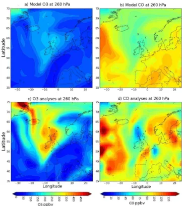
In this section, we present the case study of a STE event on 15 August 2007 over the British Isles. Figure 1 shows the O3and CO fields for MOCAGE and MOCAGE-PALM (MLS O3analyses and MOPITT CO analyses) in the UTLS (260 hPa) between 35–75◦
N and 35◦
W–25◦
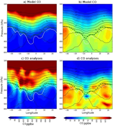
E. Figure 2 shows longitude-pressure cross sections at 59◦
N between 35◦
W and 25◦
E. These figures display the free-model run CO fields (hereafter model CO) and MOPITT CO analyses (hereafter CO analyses) and free-model run O3fields (here-after model O3) and MLS O3analyses (hereafter O3 analy-ses). The 380 K isentrope (black solid line) and the 2 PVU (white solid line) contours define the LMS height range. The STE event shows a deep stratospheric intrusion with high O3 values (low CO values) coming from polar latitudes spread-ing southward over western Europe.
In the latitude–longitude maps, O3analyses (Fig. 1c) show increased values in the STE structure compared to the model. Conversely, CO analyses (Fig. 1d) tend to exhibit decreased values in the STE structure compared to the model and also increased values around the STE. Along the vertical, O3 anal-yses (Fig. 2c) show increased O3 in the 200–300 hPa layer compared to the model O3 field. For CO analyses, a mini-mum of CO in the cross section (Fig. 2d) is in good agree-ment with the stratospheric intrusion (between 10 and 0◦
W) down to 400 hPa. At the LMS height range and at longi-tudes around the intrusion, the CO assimilated fields also dis-play higher values than the model CO fields. LEA2010 also
Fig. 1.Longitude–latitude maps at 260 hPa of model O3(a), model
CO(b), O3analyses(c)and CO analyses(d)for 15 August 2007 at
12:00 UTC.
showed that CO analyses and O3analyses are in better agree-ment with independent data (MOZAIC flights, WOUDC ozone sondes and remotely sensed data) than the free-model run. A perspective of LEA2010 was to focus on the quantifi-cation of the contribution of O3and CO assimilated species in the chemical mixing process between the stratosphere and the troposphere. In a CTM context, none of the meteoro-logical fields are modified and only the chemical fields are modified, through the assimilation process. The ExTL diag-nosed in this study is then the layer characterizing the chem-ical transition. In this study, we diagnose how this chemchem-ical transition, i.e., an estimate of the ExTL, is modified through the different assimilation experiments. By modifying only the chemical fields, the air mass mixing itself is not mod-ified by the assimilation, but the diagnosed mixing process using the chemical tracer–tracer relationship is. When we re-fer to mixing in the text it is about diagnosed mixing using the chemical fields. To quantify the contribution of each ex-periment presented here, we have used the three diagnostics discussed by Pan et al. (2007):
1. O3–CO correlations: to empirically select the CO and O3 values that belong to the stratosphere, the tropo-sphere and the ExTL.
Fig. 2.Zonal cross sections at 59◦N between 40◦W and 40◦E
lon-gitude and between 600 and 100 hPa in the vertical for model O3
(a), model CO(b), O3analyses(c)and CO analyses(d). The white
line corresponds to the 2 PVU contour. The black lines correspond to the 300 to 400 K isentropic contours by 10 K intervals. The line with green circles corresponds to the thermal tropopause. Panels are for 15 August 2007 at 12:00 UTC.
wave activity and to diagnose the effect of data assimi-lation on the UTLS CO and O3gradients.
3. Sharpness of the transition: to quantify the depth and the location of the ExTL.
3.1 Diagnostic 1: O3–CO correlations
Tracer–tracer correlation methods help to identify the chem-ical transition between the stratosphere and the troposphere and the mixing processes in the LMS (Fischer et al., 2000; Zahn et al., 2000; Hoor et al., 2002, 2004; Pan et al., 2004, 2007). Tracer–tracer correlation methods are effective to di-agnose mixing in the ExTL. These methods follow an em-pirical process to select the tropospheric values, transition layer values and stratospheric values. It is also important to know that the diagnostic would give different results if differ-ent tracers are used, for example O3–H2O correlations (Heg-glin et al., 2009). In this section, we use O3–CO correlations to determine empirically the chemical transition layer from model and analyzed fields. Diagnosing the chemical transi-tion layer using O3–H2O is out of the scope of this paper since H2O has not been assimilated. Figure 3 shows the O3–
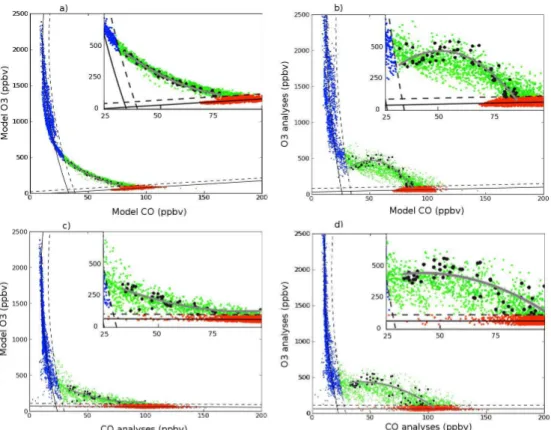
CO relationships for model O3vs. model CO (Fig. 3a), O3 analyses vs. model CO (Fig. 3b), model O3vs. CO analyses (Fig. 3c) and O3analyses vs. CO analyses (Fig. 3d). As de-scribed by Pan et al. (2007), the O3–CO relationship is “L” shaped and has a stratospheric branch (high O3 values and low CO values) and a tropospheric branch (low O3 values and high CO values). These two branches can be represented by an approximate quasi-linear relation between O3and CO. Between these two branches the relationship between O3and CO is nonlinear due to the different chemical composition of the stratosphere and the troposphere.
We have applied the O3–CO correlation diagnostic on 15 August 2007 12:00 UTC between 30◦
W–10◦
E and 40– 65◦
N where the STE takes place. We have also applied the diagnostics in the 700–80 hPa vertical range to avoid the boundary layer values and the high stratospheric ozone values. The stratospheric branch, where high O3variability and low CO variability are observed, is empirically identi-fied with a selection criterion defined by Pan et al. (2007). In Fig. 2, low CO values are mainly located in the strato-sphere (above the 380 K isentrope) in the MOCAGE CO and in the MOPITT CO analyses. A quadratic fit is done with the CO values less than 25 ppbv. CO values that are below+3σ (whereσ is the standard deviation of the selected data) from
the fit are considered as stratospheric (blue dots in Fig. 3). The tropospheric branch, where low O3variability and high CO variability are observed, is also empirically identified with a selection criterion defined by Pan et al. (2007). In Fig. 2, these low O3 values are mainly located in the tro-posphere (below the 2 PVU line) in the MOCAGE O3 and in the MLS O3analyses. A linear fit is done with O3values lower than 70 ppbv. O3values that are lower than +3σ from
the fit are considered as tropospheric (red dots in Fig. 3). Be-tween these two branches a set of points (green dots in Fig. 3) mark a chemical transition between the stratosphere and the troposphere.
The “L” shape is detected in the four O3–CO correla-tions, but the transition differs significantly between them. The transition is composed by mixing lines corresponding to O3–CO vertical relationships for each latitude–longitude lo-cation of the model. To illustrate this concept we have plotted in black the points located between 20 and 0◦
W on the 59◦
Fig. 3.Comparisons of the O3–CO relationships between model O3vs. model CO(a), O3analyses vs. model CO(b), model O3vs. CO
analyses(c)and O3analyses vs. CO analyses(d)in the area between 30◦W–10◦E and 40–65◦N on 15 August 2007 at 12:00 UTC. In
all cases, red and blue dots are identified as tropospheric and stratospheric model grid points, respectively. Black solid lines indicate fits to
tropospheric and stratospheric values and the dashed lines are the+3σ values (whereσis the standard deviation of the selected data) from
those fits. The green dots are identified as the transition between stratospheric and tropospheric air. The transitional points between 20 and
0◦W on the 59◦N vertical plane are in black and are fitted by the gray line (see text for details). Within each plot box a zoom of the transition
layer is provided (top right) on each panel.
transition indicates a rapid mixing of tropospheric and strato-spheric air masses. In our case study, the convex curvature di-agnosed in the O3–CO correlations does not indicate a rapid mixing process as expected in a STE.
Following Plumb (2007) the compactness of the tracer– tracer correlation is proportional to the variation of the chem-ical fields along isentropic surfaces. In the case of the free-model run and in the region of interest, the chemical vari-ability at tropopause altitudes is relatively low following the isentropic lines (see Fig. 2a and b). This low variability is diagnosed by a compact correlation between O3and CO val-ues in the transition layer. The dots located in the transition region are merged in the same slope, indicating the same be-havior of the O3–CO correlations at different locations. Hoor et al. (2002) also suggests that mixing occurring only episod-ically, or involving very different tropospheric air masses (e.g., rather different CO concentrations), would spread the compact relationship in the transition layer. Then the low spread in the O3–CO correlations observed here suggests a low mixing activity represented by the model during the STE.
Compared to the model O3vs. model CO correlations, the O3analyses vs. model CO correlations show an increase of O3 values in the chemical transition. The relationship be-tween O3analyses and model CO (Fig. 3b) is less compact, showing different shapes of mixing lines at different loca-tions. This illustrates the O3variability following the isen-tropes induced by MLS assimilation at tropopause altitudes (see Fig. 2c). As mentioned above, a less compact O3–CO re-lationship corresponds to a mixing process occurring episod-ically. Some of the the mixing lines show a strong “concave” shape owing to the stratospheric air mass intruding the tropo-sphere, characterized by high ozone mixing ratio values. In Fig. 2c, a maximum of ozone is observed between 200 and 250 hPa and between 20 and 0◦
Table 1.Fitting coefficients for the ExTL of O3–CO correlations, assuming a quadratic formy=a2x2+a1x+a0. CO and O3values are
defined byxandy, respectively.
a2 a1 a0
model O3vs. model CO 9.73×10⁻² −1.78×101 9.11×10²
O3analyses vs. model CO −2.99×10⁻¹ 3.07×101 −3.17×10²
model O3vs. CO analyses 5.31×10⁻² −9.75 5.77×10²
O3analyses vs. CO analyses −8.84×10⁻² 7.39 2.80×10²
The model O3vs. CO analyses correlations (Fig. 3c) show a more angular “L” shape and a less compact relationship than model O3vs. model CO correlations. The assimilation process induces a less compact relationship that is due to the increased variability of the upper tropospheric CO values. As mentioned above, this suggests more diagnosed mixing between the stratosphere and the troposphere. In the MO-PITT analyses, the CO values are more variable following the isentropes. In this case CO values are decreased in the chemical transition and tend to be increased in the upper tro-posphere except in the location of the intrusion where CO values are decreased (see Fig. 2d). In general, mixing lines tend to be pulled toward the lower-left corner, corresponding to less mixing. At the location of the intrusion, the relation-ship is the less curved, and the slope of the fit is decreased compared to the model O3vs. model CO fit (see Table 1).
In this comparison (i.e., model O3vs. CO analyses), only CO fields are assimilated, and O3 fields are not. As diag-nosed for O3analyses vs. model CO correlations, the CO an-alyzed fields are then not chemically consistent with model O3fields. However, correlation plots do not show a specific “concave” curve fit because a tropospheric CO product (MO-PITT CO) is assimilated. Even if CO is decreased in the lo-cation of the intrusion and increased around it (Fig. 2d), the dots in the correlation plot will only move in the CO dimen-sion. The MOPITT sensitivity is mainly tropospheric, and detects the intrusion as a minimum of CO visible in the anal-yses between 300 and 400 hPa and between 20 and 0◦
W (Fig. 2d) (where the dynamical tropopause is the lowest in height). Unlike the O3analyzed fields, no drastic changes can be noted in the CO analyzed fields in the lower stratosphere (around 360 K and 380 K levels). For this reasons, MOPITT CO analyses do not modify significantly the curvature of the mixing lines.
The O3analyses vs. CO analyses correlations show both the effect of MLS O3analyses and MOPITT CO analyses. In the chemical transition, O3values are increased whereas CO values are decreased. The spread of the O3–CO correlations in the chemical transition is increased compared to the other O3–CO correlations, showing an increased spatial variability of the O3–CO mixing lines. At the location of the intrusion the mixing lines still show a concave shape but with a slight curvature compared to the O3analyses vs. model CO mixing lines (see Table 1). This is due to a better O3–CO
consis-tency when both species are assimilated than when only one is assimilated. In this section, we use O3–CO correlations to select empirically the chemical transition points in order to have an estimate of the ExTL. The impact of assimilation of O3and CO fields on the correlations is discussed. We also diagnose in the next sections how the assimilation of MO-PITT CO and MLS O3data affects the spatial extent of the estimated ExTL.
3.2 Diagnostic 2: profile comparisons using relative altitude coordinates
In the second diagnostic, we analyze the tracer behavior in al-titude coordinates relative to a chosen tropopause level. Be-cause rapid changes in height of tracer concentrations hap-pen near the tropopause, it is helpful to use a tropopause-relative vertical coordinate to reduce the geophysical vari-ability caused by wave activity at synoptic and planetary scales. The thermal tropopause has been used as a reference level by Pan et al. (2007) and Pan et al. (2004) to calcu-late relative altitudes. The thermal tropopause and the dy-namical tropopause can provide double thermal or dynami-cal tropopause features related to Rossby-wave breaking pro-cesses and associated transport (Pan et al., 2009; Homeyer et al., 2010). These double tropopause structures lead to dif-ficulties in calculating diagnostics and in their interpretation. Figure 2 displays the location of the lower values of the ther-mal tropopause (green circles). We then choose the lowest levels of the thermal tropopause as reference level to calcu-late relative altitudes.
Fig. 4.O3and CO profiles in the region between 30◦W–10◦E and 40–65◦N on 15 August 2007 at 12:00 UTC. O3profiles (ppbv) in altitude
coordinates (km) relative to the 360 K level are provided for model O3vs. model CO(a), O3analyses vs. model CO(b)and O3analyses
vs. CO analyses(c). CO profiles (ppbv) in relative altitude coordinates (km) are provided for model O3vs. model CO(d), model O3vs.
CO analyses(e)and O3analyses vs. CO analyses(f). Following selection criteria, red and blue dots are identified as of tropospheric and
stratospheric origin, respectively. The green dots are identified as the transitional layer between the stratosphere and the troposphere (see text
for details). Black lines represent the mean profile every kilometer, and horizontal error bars show the 1σ standard deviation.
run simulations the upper and lower boundaries of the esti-mated ExTL are diagnosed at approximatively 3 and−1 km, respectively (Fig. 4a and d). Positive and negative altitudes are below and above the thermal tropopause, respectively. Compared to the free-model run, O3analyses (Fig. 4b) show more O3 in the ExTL (green dots) and in the troposphere (red dots). In relative altitude, the estimated ExTL extends into the troposphere to−3 km. The upper boundary height is not significantly modified but the lower boundary is lowered by 2 km. It has been shown that the tropospheric O3 con-centrations in MLS analyses (with MOCAGE) are increased due to downward transport during the STE event (Barr´e et al., 2012). Thus, some increased upper tropospheric O3 values are greater than the tropospheric threshold defined in Sect. 3.1. In the CO profiles, analyses (Fig. 4e) show values greater than the values of the free run in the troposphere and lower than the values of the free run in the stratosphere. This leads to a stronger CO gradient in the ExTL around the ther-mal tropopause. This stronger gradient does not give a sig-nificantly narrower extent of the ExTL boundaries in RALT coordinates. The location of the estimated ExTL boundaries could differ significantly in the RALT space depending on O3 analyses, and CO analyses are used separately or together. When O3analyses and CO analyses are used together in the diagnostics (Fig. 4c and f), the heights of the boundaries are close to those found on O3analyses and model CO. In the
next section, we further examine in detail the estimated ExTL distributions in the RALT space.
3.3 Diagnostic 3: sharpness of the transition
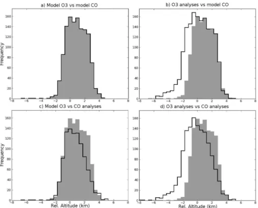
The third diagnostic provides the distribution of the esti-mated ExTL in relative altitude space (as defined in Sects. 3.1 and 3.2). The shape of the estimated ExTL distribution will allow for us to quantify its location and depth. Figure 5a–d displays the distributions for the various O3–CO relation-ships: model O3vs. model CO, O3analyses vs. model CO, model O3vs. CO analyses and O3analyses vs. CO analyses, respectively. Table 2 provides the heights of the mean and the standard deviation of the estimated ExTL distributions in relative altitude space. The free-model run distribution has its mean height at 1.42 km above the thermal tropopause with a standard deviation of 1.3 km. Studies using in situ aircraft measurement show that the ExTL is centered on the thermal tropopause with a narrower extent than observed in this study (Pan et al., 2004, 2007). In a multi-model assessment, Heg-glin et al. (2010) showed that models simulate an ExTL that is wider than observed in satellite observations, and shifted above the thermal tropopause. The low vertical resolution (800 m) in the model UTLS layers and also the low hori-zontal resolution (2◦×
2◦
Table 2.Heights of the mean, median and standard deviation of the ExTL distribution in relative altitude space (km) for the different experiments. Negative mean values and positive mean values are below and above the thermal tropopause, respectively.
Mean Standard Deviation
model O3vs. model CO 1.15 1.29
O3analyses vs. model CO 0.45 1.74
model O3vs. CO analyses 0.93 1.28
O3analyses vs. CO analyses 0.16 1.70
the tropopause. This results in a broad transition layer in the UTLS. Thus, in our case, a narrower and a lower altitude distribution would be considered as benefits from the data assimilation.
Compared to the model O3 vs. model CO distribution, the O3 analyses vs. model CO distribution shows an in-creased spread with a standard deviation of 2 km (Fig. 5b and Table 2) but a lower mean value of about 0.45 km. As described in Sect. 3.2, an increase of tropospheric O3 val-ues leads to a broadening of the estimated ExTL (down to RALT= −4 km) in the troposphere. No significant changes in the stratosphere (positive RALT values) of the distribution can be noted. The increase of O3 in the upper troposphere leads to increase of the estimated ExTL depth toward neg-ative RALT. Due to the low sensitivity of the stratospheric selection criterion to the O3variations, the stratospheric side of the estimated ExTL is not significantly modified. How-ever, the STE is detected by the tropospheric selection crite-rion, and the distribution becomes skewed toward negative RALT coordinates. Pan et al. (2004) showed that skewed distributions, particularly toward negative relative altitudes, indicate active mixing from the stratosphere to the tropo-sphere. Validation against independent measurements as in Barr´e et al. (2012) and LEA2010 shows that UTLS ozone fields are improved by MLS assimilation, and the overall ef-fect of MLS assimilation is to increase the LMS ozone fields. Barr´e et al. (2012) also show that MLS assimilation incre-ments in the lower stratosphere are transported into the tro-posphere during STE events. This impacts the trotro-posphere by increasing its ozone mixing ratio. According to these pre-vious studies, MLS analyses induce a more intense ozone mixing between the stratosphere and the troposphere. This ozone mass mixing should not to be confused with the air mass mixing, which is not changed in a CTM context. The skewed shape of the distribution then indicates this more in-tense ozone mixing from the stratosphere to the troposphere in MLS O3 analyses than in the free-model run. Despite a wider spread of the estimated ExTL distribution, the O3 anal-yses vs. model CO ExTL distribution shows a mean height closer to the thermal tropopause than the model O3vs. model CO ExTL distribution. This is consistent with Fig. 2c, where the height of ozone gradient in the O3analyses have a better match with the thermal tropopause height.
Compared to model O3vs. model CO distributions and the O3analyses vs. model CO distributions, the model O3vs. CO analyses provides a narrower estimated ExTL (Fig. 5c). The means of the distributions are reduced compared to model O3vs. model CO distribution, but not as much as for the O3 analyses vs. model CO (see Table 2). The standard deviation is very slightly reduced (by 0.01 km). Compared to the free-model run, CO analyses increase CO concentrations in the upper troposphere around the STE. However, at the location of the intrusion, the reduced CO values in the upper tropo-sphere are not detected by the tropospheric selection crite-rion (described in Sect. 3.1), which is not very sensitive to CO variations. Moreover, the stratospheric selection criterion is highly sensitive to CO variations. Compared to the model O3vs. model CO, the spread of the model O3vs. CO analy-ses distribution is reduced in the stratospheric side (positive RALT), whereas the tropospheric side (negative RALT) is not significantly modified. This lowers the mean value of the distribution.
The O3 analyses vs. CO analyses distributions (Fig. 5d) have the same shape as the model O3 vs. model CO distri-bution but are not narrowed. The mean of the distridistri-bution is very close to the thermal tropopause (0.16 km). The standard deviations are slightly lower than those of the O3analyses vs. model CO distributions but larger than those of the model O3 vs. model CO distributions. The estimated ExTL distribution benefits from the combination of the information provided by O3analyses and CO analyses. CO analyses reduce the es-timated ExTL distribution extent on its the stratospheric side and O3analyses increase the estimated ExTL distribution ex-tent on its tropospheric side.
Pan et al. (2004) found using aircraft measurements that the center of the ExTL is statistically associated with the ther-mal tropopause, and the thickness of this layer is∼2–3 km in the midlatitudes. In Table 2, the thickness of the estimated ExTL is∼3 km (2σ), and the mean and median values are
lowered by∼1 km. Moreover, because of the rapid overturn-ing of air masses in the troposphere and high static stabil-ity in the stratosphere, stratosphere-to-troposphere transport (STT) shows deeper signatures in altitude than troposphere-to-stratosphere transport (TST) (Hoor et al., 2002). Conse-quently, during STT events, the ExTL will show a skewed distribution toward negative RALT. This skewed distribution is only seen with O3 analyses, which provide increased O3 values in the LMS and below (see for example Fig. 2c) and allow for detection of the appropriate STT in these diagnoses. Data assimilation of stratospheric O3limb measurements makes the following possible:
Fig. 5.Histograms showing the distributions of the ExTL in relative altitude space in the region between 30◦W–10◦E and 40–65◦N on 15
August 2007 at 12:00 UTC. model O3vs. model CO(a), O3analyses vs. model CO(b), model O3vs. CO analyses(c)and O3analyses vs.
CO analyses(d)are displayed in black, and model O3vs. model CO distribution is overplotted in gray on the plots. The histograms display
the absolute frequencies.
ii. It increases the ozone mixing ratio in the upper tropo-sphere (Barr´e et al., 2012), resulting in an increase of the ExTL distribution spread.
Data assimilation of tropospheric CO nadir measurements has the following effects:
i. It does not allow for detection of deep stratospheric sig-natures as efficiently as O3 limb measurements. The ExTL distribution is not significantly lowered and not skewed.
ii. It improves the upper tropospheric CO fields (see val-idation in LEA2010), providing a sharper CO gradient in the UTLS and narrowing the ExTL distribution in its stratospheric side.
4 Global ExTL for the month of August 2007
In this section, we apply the diagnostic of Sect. 3.3 (sharp-ness of the transition) on the global scale in order to inves-tigate the impact of data assimilation of MOPITT CO and MLS O3on the estimated ExTL. Because the STE activities near the extratropical tropopause are largely associated with synoptic scale dynamical processes that are on a timescale of a few days to a week, the variability in tracer fields induced
by these activities is largely smoothed out in the monthly mean fields. The diagnostics have been then performed on the 15 August 2007 12:00 UTC fields and on the monthly time-averaged (August 2007) fields. The diagnostics are ap-plied on 10◦
S latitude bands and regression selection crite-ria take into account every latitude–longitude grid point in those latitude bands. We also only consider extratropical lati-tudes outside the 20◦
S–20◦
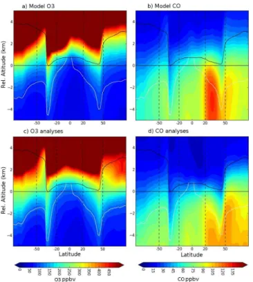
N range. Figure 6a–d show zonal means of the model O3, model CO, O3analyses and CO anal-yses for the month of August 2007 (i.e., longitude-time av-erage), in tropopause-relative altitude coordinates. The lower white line is the 2 PVU level and the upper black line is the 380 K isentrope, denoting the LMS bounds. In general, O3 analyses increase the amount of O3in the LMS, especially at northern extratropical latitudes poleward of 50◦
N (by more than 200 ppbv). CO analyses increase the tropospheric CO values, except between 20 and 40◦N, and decrease the lower
stratospheric CO values.
We estimate the distribution of the O3–CO ExTL for lat-itude bands of 10◦
between 90 and 20◦
S and between 20 and 90◦
Fig. 6.Zonal averages for the month of August 2007 in relative
alti-tudes (km) of model O3(a), model CO(b), O3analyses(c)and CO
analyses(d). Dashed black vertical lines mark the regions of interest
(i.e., 90–50◦S, 50–20◦S, 20–50◦N and 50–90◦N). The lowermost
stratosphere bounds are represented by the 2 PVU contour in abso-lute value (lower white line), and the 380 K isentrope (upper black line).
deviation from the mean (light green lines) in RALT coor-dinates. The LMS bounds (the lower blue line is the 2 PVU level and the upper blue line is the 380 K isentrope) and the thermal tropopause (straight horizontal line) are also over-plotted in RALT coordinates. The estimated ExTL distribu-tions are provided for the four experiments: model O3 vs. model CO, O3 analyses vs. model CO, model O3 vs. CO analyses and O3analyses vs. CO analyses. Tables 3 and 4 provide mean and standard deviation values for four regions – 90 to 50◦S, 50 to 20◦S, 20 to 50◦N and 50 to 90◦N –
as defined by the dashed lines in the Figs. 7 and 8, respec-tively. The standard deviations are systematically higher in the distributions calculated from the 15 August 2007 (here-after daily diagnostics) than in the distributions calculated from the monthly averaged (August 2007) fields (hereafter monthly diagnostics). As mentioned above, the variability as-sociated with STE activities located at extratropical latitudes is smoothed out in the monthly means fields. This results in a narrower ExTL distribution estimate when a monthly mean field is used. However, the diagnostic on the monthly mean fields is useful to diagnose the behavior on the global esti-mated ExTL during the month of August 2007.
Fig. 7.Latitudinal height variations in altitude coordinates (km)
rel-ative to the 360 K level of the ExTL distribution for model O3vs.
model CO(a), O3analyses vs. model CO (b), model O3 vs. CO
analyses(c)and O3analyses vs. CO analyses(d)calculated from
the 15 August 2007 12:00 UTC tracer fields. Red-filled contours provide the decile altitudes of the distribution. Red and green lines are the median and mean altitudes, respectively. Blue lines show the lowermost stratosphere bounds: the lower line provides the 2 PVU contour in absolute value, while the upper line provides the 380 K isentropic contour.
In the model O3vs. model CO distributions, the estimated ExTL has latitudinal variations in the RALT space (Figs. 7a and 8a). In the Southern Hemisphere, the estimated ExTL follows the 2 PVU line (mean and median values), although 1.5 to 2 km above it. In the Southern Hemisphere the mean and median values of the estimated ExTL are located around the thermal tropopause. The estimated ExTL is located on negative RALT near the South Pole, positive RALT at the midlatitudes and RALT close to 0◦
at the subtropics. This variation of altitudes is more visible on distributions calcu-lated with daily diagnostics than with monthly diagnostics for reasons mentioned above (the fields are smoothed). In the Northern Hemisphere the location of the estimated ExTL is found above the thermal tropopause by 1 to 2 km. Between 20 and 50◦N the estimated ExTL is located at 0.8 and 0.6 km
for daily and monthly diagnostics, respectively (Tables 3 and 4 ). Between 50◦
N and the North Pole the estimated ExTL is located at 2 and 1.9 km for daily and monthly diagnostics, respectively (Tables 3 and 4).
Table 3.Heights of the mean and standard deviation of the ExTL distribution in relative altitude space (km) for the different experiments and for the different latitude bands over the globe, calculated from 15 August 2007 12:00 UTC tracer fields. Negative and positive mean values are below and above the thermal tropopause, respectively.
90–50◦S 50–20◦S 20–50◦N 50–90◦N
model O3vs. model CO
Mean 0.072 0.727 0.800 2.062
Standard Deviation 1.195 1.913 1.555 1.467
O3analyses vs. model CO
Mean −0.200 0.432 0.208 1.157
Standard Deviation 1.342 2.060 1.962 1.969
model O3vs. CO analyses
Mean 0.106 0.403 0.036 1.466
Standard Deviation 1.187 1.747 1.283 0.986
O3analyses vs. CO analyses
Mean −0.240 0.076 −0.660 0.503
Standard Deviation 1.290 1.941 1.714 1.648
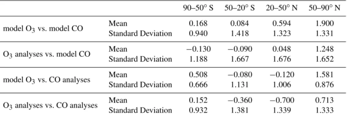
Table 4.Heights of the mean and standard deviation of the ExTL distribution in relative altitude space (km) for the different experiments and for the different latitude bands over the globe, calculated from monthly average (August 2007) tracer fields. Negative and positive mean values are below and above the thermal tropopause, respectively.
90–50◦S 50–20◦S 20–50◦N 50–90◦N
model O3vs. model CO
Mean 0.168 0.084 0.594 1.900
Standard Deviation 0.940 1.418 1.323 1.331
O3analyses vs. model CO
Mean −0.130 −0.090 0.048 1.248
Standard Deviation 1.188 1.667 1.676 1.652
model O3vs. CO analyses
Mean 0.508 −0.080 −0.120 1.581
Standard Deviation 0.666 1.131 1.006 0.876
O3analyses vs. CO analyses
Mean 0.152 −0.360 −0.700 0.713
Standard Deviation 0.932 1.381 1.339 1.333
diagnostic, a wider extent of the estimated ExTL corresponds to a tendency of deeper exchanges between the stratosphere and the troposphere. The wider extent of the estimated ExTL in the Northern Hemisphere can be interpreted at the global scale as more intense STE activity. Two maxima of estimated ExTL thickness are also identified in both hemispheres near 35◦
S and 35◦
N, corresponding to the location of the sub-tropical jets where mixing processes occur (Gettelman et al., 2011). Pan et al. (2004) deduced from aircraft observations (in the Northern Hemisphere) of O3 and CO an ExTL cen-tered at the thermal tropopause with a thickness between 2 and 3 km expanding into a thicker layer in the vicinity of the subtropical jet.
The O3 analyses vs. model CO data provides slightly wider distributions for the estimated ExTL for all latitudes (Figs. 7b and 8b) with a standard deviation that is increased by up to 0.5 km (between 50◦
N and the North Pole). When stratospheric O3 profiles are assimilated, the model is un-able to improve the strong O3 gradients observed in the UTLS. These wider distributions also suggest a more intense O3 mixing produced by MLS assimilation. As explained in Sect. 3.3, MLS assimilation increments that increase O3
in the LMS are advected through the tropopause and then increase the O3 mixing. O3 analyses move the estimated ExTL location to lower altitudes and always have median and mean values of the distribution below the 380 K level. The mean values of the distributions are significantly low-ered in the Northern Hemisphere by−0.6 km in the subtrop-ics and by−0.9 km in the middle and polar latitudes closer to the thermal tropopause. In the Southern Hemisphere the estimated ExTL mean location is not lowered as much (less than 0.1 km) than in the Northern Hemisphere. This is can be explained by a significant increase of ozone in the LMS in the Northern Hemisphere but not in the Southern Hemisphere (Fig. 6c). Model O3vs. CO analyses (Figs. 7c and 8c) show reduction in the estimated ExTL thickness. The layer thick-ness is strongly reduced, as reflected in a reduction of the standard deviation by about−0.38 km in the Northern Hemi-sphere and by −0.18 km in the Southern Hemisphere. The mean and the median values match the thermal tropopause poleward of 50◦
S but remain 1.5 to 2 km above the thermal tropopause poleward of 50◦
N.
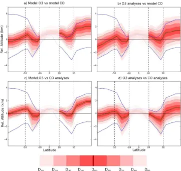
Fig. 8.Latitudinal height variations in altitude coordinates (km)
rel-ative to the 360 K level of the ExTL distribution for model O3vs.
model CO(a), O3analyses vs. model CO (b), model O3vs. CO
analyses(c)and O3analyses vs. CO analyses(d)calculated from
the monthly mean tracer fields on August 2007. Red-filled contours provide the decile altitudes of the distribution. Red and green lines are the median and mean altitudes, respectively. Blue lines show the lowermost stratosphere bounds: the lower line provides the 2 PVU contour in absolute value, the upper line provides the 380 K isen-tropic contour. Tropical latitudes are not shown.
previously described distributions (i.e., O3 analyses vs. model CO distribution and model O3vs. CO analyses distri-bution). The standard deviations are not reduced, and show very similar values to those from model O3 vs. model CO distributions (see Tables 3 and 4). In a general manner, the most significant changes in the estimated ExTL distributions are located in the Northern Hemisphere. The location of the estimated ExTL is lowered close to the thermal tropopause (due to O3 analyses), and the spread of the distributions is conserved (due to CO analyses). No significant changes can be noted in the Southern Hemisphere, except near the South Pole in the daily distributions. In the subtropical lati-tudes, the estimated ExTL is located 1 km below the thermal tropopause. This region is subject to the thermal tropopause break at the location of the subtropical jet providing an in-stance of a double tropopause. It has been shown that the ExTL, at these latitudes, has a contribution from the subtrop-ical jet, the tropsubtrop-ical tropopause layer and the midlatitudes lowermost stratosphere, forming complex structures in the ExTL as double thermal tropopause features (Vogel et al., 2011). In this study, only the lower thermal tropopause al-titudes have been taken in account to perform the diagnos-tics. At subtropical latitudes, the ExTL distribution could
be more centered on the higher thermal tropopause occur-rence, where strong tropospheric-to-stratospheric intrusions from the tropical tropopause layer are existent. This could impact the diagnostics providing shifted ExTL distribution on positive RALT.
In this section, we have shown the impacts of data assim-ilation on the the ExTL representation between the strato-sphere and the tropostrato-sphere at a global scale in the extrat-ropics. Due to the shape of the O3–CO relationship and the selection criteria described in Sect. 3.1, the upper bound of the ExTL distribution is mostly sensitive to CO variations, whereas the lower bound of the ExTL distribution is mostly sensitive to O3variations. CO analyses have more influence on the stratospheric side of the estimated ExTL and reduce the mixing layer depth. O3 analyses have more influence on the tropospheric side of the estimated ExTL and are not able to reduce the estimated ExTL depth but have the ca-pability to represent deeper STE signatures at extratropical latitudes. This lowers the location of the estimated ExTL closer to the thermal tropopause. A combination of these two analyses shows significantly better results than each analy-sis separately: the estimated ExTL location matches the ther-mal tropopause location at middle and polar latitudes, and its spread is in the range of what is observed by in situ and satellite measurements studies. In the Northern Hemisphere, Pan et al. (2004) deduced from aircraft observations that the ExTL thickness is 2–3 km at midlatitudes, with enhanced values in the vicinity of the subtropical jet. In Tables 3 and 4, the O3analyses vs. CO analyses distribution shows a stan-dard deviation (2σ) in a range from∼2.7 to∼3.4 km be-tween 50 and 90◦N. Hegglin et al. (2009) found in satellite
measurements an ExTL depth in extratropical latitudes be-tween 1.5 and 4 km that matches our results.
5 Discussions and conclusions
of different tracers (e.g., from the same atmospheric sounder) provide a better consistency in the tracer–tracer relationship? In addition to diagnosing the effect of data assimilation on the O3–CO relationship, we also diagnose the ExTL estimated distribution in the relative altitude space. The free-model run O3–CO relationship shows a 2.5 km wide ExTL distribution that is centered 1 km above the ther-mal tropopause. This distribution shows the typical behav-ior of the models representing the atmospheric composition, namely an overestimation of the ExTL depth and of its lo-cation in height, above the thermal tropopause. MLS O3 analyses extend the spread of the distribution toward tro-pospheric altitudes due to an increase of O3 values in the UTLS. This increases the depth of the ExTL by about 1 km and lowers the mean location by 0.7 km closer to the ther-mal tropopause. The estimated ExTL distribution is skewed toward tropopause-relative altitudes, showing the capability of MLS O3 analyses to accentuate the ozone signature of the STE event. MOPITT CO analyses have the capability to sharpen the CO gradient in the UTLS. This slightly reduces the spread of the ExTL on its stratospheric side, showing a mean location closer to the thermal tropopause. Due to the low sensitivity to CO tropospheric variations of the diagnos-tics used in the present study, MOPITT CO analyses do not show a signature of STE in the estimated ExTL distributions. In combining the information provided by MLS O3 analy-ses and MOPITT CO analyanaly-ses, the estimated ExTL distri-bution has a more realistic shape and location. The ExTL mean location is centered on the thermal tropopause, but the spread of the ExTL is increased compared to the free-model run. It has been shown that models simulate an ExTL deeper than observed in aircraft measurements, and shifted above the thermal tropopause (Hegglin et al., 2010). This is due to the limited vertical and horizontal resolutions of the models, as well as the lack of representativeness in the aircraft ob-servations. However, data assimilation of CO and O3 satel-lite measurements helps to improve the representation of the ExTL, and tries to overcome the limitation due to the rela-tively low model resolution.
We also extend the diagnostics at global extratropical lat-itudes for the August 2007 time period. MLS O3 analyses show a spread of the estimated ExTL distribution toward the surface, which lowers its mean location closer to the ther-mal tropopause. MOPITT CO analyses reduce the spread of the estimated ExTL on its stratospheric side, which also low-ers its mean location closer to the thermal tropopause. When MLS O3 analyses and MOPITT CO analyses are used to-gether, a synergistic effect is observed. The ExTL location poleward of 50◦
N and 50◦
S matches the thermal tropopause, and the depth of the estimated ExTL is conserved compared to the free-model run O3–CO diagnostics. As shown in the case study, the STE is characterized by the tropospheric ex-tent of the ExTL. In the global diagnostics, MLS O3analyses increase the tropospheric extent of the ExTL distribution be-low the 2 PVU level, showing a more intense O3mixing from
stratosphere to troposphere. Further investigation is needed, for example using O3 and CO fields analyses over longer timescales (e.g., more than 1 yr) to diagnose the seasonal be-havior of the ExTL.
Acknowledgements. We thank the reviewers for their constructive comments that helped to improve the article. We thank the Jet Propulsion Laboratory MLS science team for retrieving and
providing the O3 MLS data. We thank the National Center for
Atmospheric Research MOPITT science team and NASA for producing and archiving the MOPITT CO product. This work was funded by the Centre National de Recherches Scientifiques (CNRS) and the Centre National de Recherches M´et´eorologiques (CNRM) of M´et´eo-France. V.-H. Peuch, J.-L. Atti´e, L. El Amraoui and W. A. Lahoz are supported by the RTRA/STAE (POGEQA project). J.-L. Atti´e thanks also the R´egion Midi Pyr´en´ees (INFOAIR project).
Edited by: M. Palm
The publication of this article is financed by CNRS-INSU.
References
Barr´e, J., Peuch, V.-H., Atti´e, J.-L., El Amraoui, L., Lahoz, W. A., Josse, B., Claeyman, M., and N´ed´elec, P.: Stratosphere-troposphere ozone exchange from high resolution MLS ozone analyses, Atmos. Chem. Phys., 12, 6129–6144, doi:10.5194/acp-12-6129-2012, 2012.
Barret, B., Ricaud, P., Mari, C., Atti´e, J.-L., Bousserez, N., Josse, B., Le Flochmo¨en, E., Livesey, N. J., Massart, S., Peuch, V.-H., Piacentini, A., Sauvage, B., Thouret, V., and Cammas, J.-P.: Transport pathways of CO in the African upper troposphere during the monsoon season: a study based upon the assimilation of spaceborne observations, Atmos. Chem. Phys., 8, 3231–3246, doi:10.5194/acp-8-3231-2008, 2008.
Bechtold, P., Bazile, E., Guichard, F., Mascart, P., and Richard, E.: A mass-flux convection scheme for regional and global models, Q. J. Roy. Meteor. Soc., 96, 869–886, 2001.
Bencherif, H., Amraoui, L. E., Sernane, N., Massart, S., Charyulu, D. V., Hauchecorne, A., and Peuch, V.-H.: Examination of the 2002 major warming in the southern hemisphere using ground-based and Odin/SMR assimilated data: stratospheric ozone dis-tributions and tropic/mid-latitude exchange, Can. J. Phys., 85, 1287–1300, 2007.
Buis, S., Piacentini, A., and D´eclat, D.: PALM: a computational framework for assembling high-performance computing appli-cations, Concurrency Computat.: Pract. Exper., 18, 231–245, doi:10.1002/cpe.914, 2006.
Courtier, P., Freydier, C., Geleyn, J. F., Rabier, F., and Rochas, M.: The ARPEGE project at M´et´eo France, in: Atmospheric Mod-els, 2, 193–231, Workshop on Numerical Methods, Reading, UK, 1991.
Drummond, J. R. and Mand, G. S.: Evaluation of operational radi-ances for the Measurement of Pollution in the Troposphere (MO-PITT) instrument CO thermal-band channels, J. Geophys. Res., 109, D03308, doi:10.1029/2003JD003970, 1996.
Dufour, A., Amodei, M., Ancellet, G., and Peuch, V.-H.: Observed and modelled ”chemical weather” during ESCOMPTE, Atmos. Res., 74, 161–189, doi:10.1016/j.atmosres.2004.04.013, 2005. El Amraoui, L., Peuch, V.-H., Ricaud, P., Massart, S., Semane,
N., Teyss`edre, H., Cariolle, D., and Karcher, F.: Ozone loss in the 2002–2003 Arctic vortex deduced from the
assimila-tion of Odin/SMR O3 and N2O measurements: N2O as a
dynamical tracer, Q. J. Roy. Meteor. Soc., 134, 217–228, doi:10.1002/qj.191, 2008a.
El Amraoui, L., Semane, N., Peuch, V.-H., and Santee, M. L.: Inves-tigation of dynamical processes in the polar stratospheric vortex during the unusually cold winter 2004/2005, Geophys. Res. Lett., 35, L03803, doi:10.1029/2007GL031251, 2008b.
El Amraoui, L., Atti´e, J.-L., Semane, N., Claeyman, M., Peuch, V.-H., Warner, J., Ricaud, P., Cammas, J.-P., Piacentini, A., Josse, B., Cariolle, D., Massart, S., and Bencherif, H.: Midlatitude
stratosphere – troposphere exchange as diagnosed by MLS O3
and MOPITT CO assimilated fields, Atmos. Chem. Phys., 10, 2175–2194, doi:10.5194/acp-10-2175-2010, 2010.
Fischer, H., Wienhold, F. G., Hoor, P., Bujok, O., Schiller, C., Siegmund, P., Ambaum, M., Scheeren, H. A., and Lelieveld, J.: Tracer correlations in the northern high latitude lowermost strato-sphere: Influence of cross-tropopause mass exchange, Geophys. Res. Lett., 27, 97–100, doi:10.1029/1999GL010879, 2000. Fisher, M. and Andersson, E.: Developments in 4D-Var and Kalman
filtering, in: Technical Memorandum Research Department, vol. 347, ECMWF, Reading, UK, 2001.
Geer, A. J., Lahoz, W. A., Bekki, S., Bormann, N., Errera, Q., Es-kes, H. J., Fonteyn, D., Jackson, D. R., JucEs-kes, M. N., Massart, S., Peuch, V.-H., Rharmili, S., and Segers, A.: The ASSET in-tercomparison of ozone analyses: method and first results, At-mos. Chem. Phys., 6, 5445–5474, doi:10.5194/acp-6-5445-2006, 2006.
Gettelman, A., Hoor, P., Pan, L. L., Randel, W. J., Heg-glin, M. I., and Birner, T.: The Extratropical Upper Tropo-sphere and Lower StratoTropo-sphere, Rev. Geophys., 49, RG3003, doi:10.1029/2011RG000355, 2011.
Hegglin, M. I., Boone, C. D., Manney, G. L., and Walker, K. A.: A global view of the extratropical tropopause transition layer from Atmospheric Chemistry Experiment Fourier Transform
Spec-trometer O3, H2O, and CO, J. Geophys. Res., 114, D00B11,
doi:10.1029/2008JD009984, 2009.
Hegglin, M. I., Gettelman, A., Hoor, P., Krichevsky, R., Manney, G. L., Pan, L. L., Son, S. W., Stiller, G., Tilmes, S., Walker, K. A., Eyring, V., Shepherd, T. G., Waugh, D., Akiyoshi, H., Anel, J. A., Austin, J., Baumgaertner, A., Bekki, S., Braesicke, P., Bruehl, C., Butchart, N., Chipperfield, M., Dameris, M., Dhomse, S., Frith, S., Garny, H., Hardiman, S. C., Joeckel, P., Kinnison, D. E., Lamarque, J. F., Mancini, E., Michou, M., Mor-genstern, O., Nakamura, T., Olivie, D., Pawson, S., Pitari, G., Plummer, D. A., Pyle, J. A., Rozanov, E., Scinocca, J. F.,
Shi-bata, K., Smale, D., Teyssedre, H., Tian, W., and Yamashita, Y.: Multimodel assessment of the upper troposphere and lower stratosphere: Extratropics, J. Geophys. Res., 115, D00M09, doi:10.1029/2010JD013884, 2010.
Holton, J. R., Haynes, P. H., McIntyre, M. E., Douglass, A. R., Rood, R. B., and Pfister, L.: Stratosphere-troposphere exchange, Rev. Geophys., 4, 403–439, 1995.
Homeyer, C. R., Bowman, K. P., and Pan, L. L.: Extrat-ropical tropopause transition layer characteristics from high-resolution sounding data, J. Geophys. Res., 115, D13108, doi:10.1029/2009JD013664, 2010.
Hoor, P., Fischer, H., Lange, L., Lelieveld, J., and Brunner, D.: Sea-sonal variations of a mixing layer in the lowermost stratosphere
as identified by the CO-O3 correlation from in situ
measure-ments, J. Geophys. Res., 107, doi:10.1029/2000JD000289, 2002. Hoor, P., Gurk, C., Brunner, D., Hegglin, M. I., Wernli, H., and Fischer, H.: Seasonality and extent of extratropical TST derived from in-situ CO measurements during SPURT, Atmos. Chem. Phys., 4, 1427–1442, doi:10.5194/acp-4-1427-2004, 2004. Jackson, D. R.: Assimilation of EOS MLS ozone observations in
the Met Office data-assimilation system, Q. J. Roy. Meteor. Soc., 133, 1771–1788, doi:10.1002/qj.140, 2007.
Josse, B., Simon, P., and Peuch, V.-H.: Radon global simulation with the multiscale chemistry transport model MOCAGE, Tel-lus, 56, 339–356, 2004.
Kalnay, E.: Atmospheric modeling, data assimilation, and pre-dictability., University Press, Cambridge, 2003.
Lahoz, W. A., Errera, Q., Swinbank, R., and Fonteyn, D.: Data as-similation of stratospheric constituents: a review, Atmos. Chem. Phys., 7, 5745–5773, doi:10.5194/acp-7-5745-2007, 2007. Lef`evre, F., Brasseur, G. P., Folkins, I., Smith, A. K., and Simon,
P.: Chemistry of the 1991–1992 stratospheric winter: three di-mensional model simulations, J. Geophys. Res., 99, 8183–8195, 1994.
Louis, J.-F.: Parametric model of vertical eddy fluxes in the atmo-sphere, Bound.-Lay. Meteorol., 17, 187–202, 1979.
Massart, S., Cariolle, D., and Peuch, V.-H.: Towards an improve-ment of the atmospheric ozone distribution and variability by assimilation of satellite data, C. R. Geosci., 337, 1305–1310, doi:10.1016/j.crte.2005.08.001, 2005.
Massart, S., Piacentini, A., Cariolle, D., El Amraoui, L., and Se-mane, N.: Assessment of the quality of the ozone measurements from the Odin/SMR instrument using data assimilation, Can. J. Phys., 85, 1209–1223, 2007.
Pan, L. L., Randel, W. J., Gary, B. L., Mahoney, M. J., and Hintsa, E. J.: Definitions and sharpness of the extratropical tropopause: A trace gas perspective, J. Geophys. Res., 109, D23103, doi:10.1029/2004JD004982, 2004.
Pan, L. L., Wei, J. C., Kinnison, D. E., Garcia, R. R., Wuebbles, D. J., and Brasseur, G. P.: A set of diagnostics for evaluating chemistry-climate models in the extratropical tropopause region, J. Geophys. Res., 112, D09316, doi:10.1029/2006JD007792, 2007.
Atmo-sph´erique `a Grande Echelle, Proceedings of M´et´eo-France work-shop on atmospheric modelling, december 1999, 33-36, 1999. Plumb, R. A.: Tracer interrelationships in the stratosphere, Rev.
Geophys., 45, RG4005, doi:10.1029/2005RG000179, 2007. Ricaud, P., Barret, B., Atti´e, J.-L., Motte, E., Le Flochmo¨en, E.,
Teyss`edre, H., Peuch, V.-H., Livesey, N., Lambert, A., and Pommereau, J.-P.: Impact of land convection on troposphere-stratosphere exchange in the tropics, Atmos. Chem. Phys., 7, 5639–5657, doi:10.5194/acp-7-5639-2007, 2007.
Semane, N., Peuch, V.-H., Amraoui, L. E., Bencherif, H., Massart, S., Cariolle, D., Atti´e, J.-L., and Abidab, R.: An observed and analysed stratospheric ozone intrusion over the high Canadian Arctic UTLS region during the summer of 2003, Q. J. Roy. Me-teor. Soc., 133, 171–178, doi:10.1002/qj.141, 2007.
Stajner, I., Wargan, K., Pawson, S., Hayashi, H., Chang, L.-P., Hud-man, R. C., Froidevaux, L., Livesey, N., Levelt, P. F., Thompson, A. M., Tarasick, D. W., Stuebi, R., Andersen, S. B., Yela, M., Koenig-Langlo, G., Schmidlin, F. J., and Witte, J. C.: Assimi-lated ozone from EOS-Aura: Evaluation of the tropopause re-gion and tropospheric columns, J. Geophys. Res., 113, D16S32, doi:10.1029/2007JD008863, 2008.
Stockwell, W. R., Kirchner, F., Khun, M., and Seefeld, S.: A new mechanism for regional atmospheric chemistry modelling, J. Geophys. Res., 102, 25847–25879, 1997.
Vogel, B., Pan, L. L., Konopka, P., Guenther, G., Mueller, R., Hall, W., Campos, T., Pollack, I., Weinheimer, A., Wei, J., Atlas, E. L., and Bowman, K. P.: Transport pathways and signatures of mixing in the extratropical tropopause region derived from Lagrangian model simulations, J. Geophys. Res., 116, D05306, doi:10.1029/2010JD014876, 2011.
Wargan, K., Pawson, S., Stajner, I., and Thouret, V.: Spa-tial structure of assimilated ozone in the upper troposphere and lower stratosphere, J. Geophys. Res., 115, D24316, doi:10.1029/2010JD013941, 2010.
Waters, J. W., Froidevaux, L., Harwood, R. S., Jarnot, R. F., Pickett, H. M., Read, W. G., Siegel, P. H., Cofield, R. E., Filipiak, M. J., Flower, D. A., Holden, J. R., Lau, G. K. K., Livesey, N. J., Man-ney, G. L., Pumphrey, H. C., Santee, M. L., Wu, D. L., Cuddy, D. T., Lay, R. R., Loo, M. S., Perun, V. S., Schwartz, M. J., Stek, P. C., Thurstans, R. P., Boyles, M. A., Chandra, K. M., Chavez, M. C., Chen, G. S., Chudasama, B. V., Dodge, R., Fuller, R. A., Girard, M. A., Jiang, J. H., Jiang, Y. B., Knosp, B. W., LaBelle, R. C., Lam, J. C., Lee, K. A., Miller, D., Oswald, J. E., Patel, N. C., Pukala, D. M., Quintero, O., Scaff, D. M., Snyder, W. V., Tope, M. C., Wagner, P. A., and Walch, M. J.: The Earth Observ-ing System Microwave Limb Sounder (EOS MLS) on the Aura satellite, IEEE T. Geosci. Remote, 44, 1075–7092, 2006. World Meteorological Organization: Scientific Assessment of
Ozone Depletion: 2002, Global ozone research and monitoring project report no. 47, 2003.