ACPD
12, 25255–25328, 2012Reactive trace gases and O3 formation in
smoke
S. K. Akagi et al.
Title Page
Abstract Introduction
Conclusions References
Tables Figures
◭ ◮
◭ ◮
Back Close
Full Screen / Esc
Printer-friendly Version Interactive Discussion
Discussion
P
a
per
|
Dis
cussion
P
a
per
|
Discussion
P
a
per
|
Discussio
n
P
a
per
|
Atmos. Chem. Phys. Discuss., 12, 25255–25328, 2012 www.atmos-chem-phys-discuss.net/12/25255/2012/ doi:10.5194/acpd-12-25255-2012
© Author(s) 2012. CC Attribution 3.0 License.
Atmospheric Chemistry and Physics Discussions
This discussion paper is/has been under review for the journal Atmospheric Chemistry and Physics (ACP). Please refer to the corresponding final paper in ACP if available.
Measurements of reactive trace gases
and variable O
3
formation rates in some
South Carolina biomass burning plumes
S. K. Akagi1, R. J. Yokelson1, I. R. Burling1, S. Meinardi2, I. Simpson2, D. R. Blake2, G. R. McMeeking3, A. Sullivan3, T. Lee3, S. Kreidenweis3, S. Urbanski4, J. Reardon4, D. W. T. Griffith5, T. J. Johnson6, and D. R. Weise7
1
University of Montana, Department of Chemistry, Missoula, MT 59812, USA
2
Department of Chemistry, University of California-Irvine, Irvine, CA 92697, USA
3
Colorado State University, Department of Atmospheric Science, Fort Collins, CO 80523, USA
4
USDA Forest Service, Rocky Mountain Research Station, Fire Sciences Laboratory, Missoula, MT 59808, USA
5
University of Wollongong, Department of Chemistry, Wollongong, New South Wales, Australia
6
Pacific Northwest National Laboratories, Richland, WA 99354, USA
7
ACPD
12, 25255–25328, 2012Reactive trace gases and O3 formation in
smoke
S. K. Akagi et al.
Title Page
Abstract Introduction
Conclusions References
Tables Figures
◭ ◮
◭ ◮
Back Close
Full Screen / Esc
Printer-friendly Version Interactive Discussion
Discussion
P
a
per
|
Dis
cussion
P
a
per
|
Discussion
P
a
per
|
Discussio
n
P
a
per
|
Received: 5 September 2012 – Accepted: 12 September 2012 – Published: 24 September 2012
Correspondence to: R. J. Yokelson ([email protected])
ACPD
12, 25255–25328, 2012Reactive trace gases and O3 formation in
smoke
S. K. Akagi et al.
Title Page
Abstract Introduction
Conclusions References
Tables Figures
◭ ◮
◭ ◮
Back Close
Full Screen / Esc
Printer-friendly Version Interactive Discussion
Discussion
P
a
per
|
Dis
cussion
P
a
per
|
Discussion
P
a
per
|
Discussio
n
P
a
per
|
Abstract
In October–November 2011 we measured trace gas emission factors from seven pre-scribed fires in South Carolina (SC), US, using two Fourier transform infrared spec-trometer (FTIR) systems and whole air sampling (WAS) into canisters followed by gas-chromatographic analysis. A total of 97 trace gas species were quantified from both
5
airborne and ground-based sampling platforms, making this one of the most detailed field studies of fire emissions to date. The measurements include the first emission factors for a suite of monoterpenes produced by heating vegetative fuels during field fires. The first quantitative FTIR observations of limonene in smoke are reported along with an expanded suite of monoterpenes measured by WAS including α-pinene,
β-10
pinene, limonene, camphene, 4-carene, and myrcene. The known chemistry of the monoterpenes and their measured abundance of 0.4–27.9 % of non-methane organic compounds (NMOCs) and∼21 % of organic aerosol (mass basis) suggests that they impacted secondary formation of ozone (O3), aerosols, and small organic trace gases such as methanol and formaldehyde in the sampled plumes in first few hours after
15
emission. The variability in the initial terpene emissions in the SC fire plumes was high and, in general, the speciation of the initially emitted gas-phase NMOCs was 13–195 % different from that observed in a similar study in nominally similar pine forests in North Carolina ∼20 months earlier. It is likely that differences in stand structure and envi-ronmental conditions contributed to the high variability observed within and between
20
these studies. Similar factors may explain much of the variability in initial emissions in the literature. The∆HCN/∆CO emission ratio, however, was found to be fairly consis-tent with previous airborne fire measurements in other coniferous-dominated ecosys-tems, with the mean for these studies being 0.90±0.06 %, further confirming the value of HCN as a biomass burning tracer. The SC results also support an earlier finding
25
ACPD
12, 25255–25328, 2012Reactive trace gases and O3 formation in
smoke
S. K. Akagi et al.
Title Page
Abstract Introduction
Conclusions References
Tables Figures
◭ ◮
◭ ◮
Back Close
Full Screen / Esc
Printer-friendly Version Interactive Discussion
Discussion
P
a
per
|
Dis
cussion
P
a
per
|
Discussion
P
a
per
|
Discussio
n
P
a
per
|
occurred in all of these plumes within two hours. The slowest O3 production was ob-served on a cloudy day with low co-emission of NOx. The fastest O3 production was observed on a sunny day when the downwind plume almost certainly incorporated sig-nificant additional NOx by passing over the Columbia, SC metropolitan area. Due to rapid plume dilution, it was only possible to acquire high-quality downwind data for two
5
other trace gas species (formaldehyde and methanol) during two of the fires. In all four of these cases, significant increases in formaldehyde and methanol were observed in <2 h. This is likely the first direct observation of post-emission methanol production in biomass burning plumes. Post-emission production of methanol does not always hap-pen in young biomass burning plumes, and its occurrence in this study could have
10
involved terpene precursors to a significant extent.
1 Introduction
On a global scale, biomass burning is thought to be the largest source of primary fine carbonaceous particles in the atmosphere and the second largest source of total trace gases (Crutzen and Andreae, 2000; Bond et al., 2004; Akagi et al., 2011). In
15
the southeastern US and to a lesser extent in other parts of the US and other coun-tries, prescribed fires are ignited to restore or maintain the natural, beneficial role that fire plays in fire-adapted ecosystems (Biswell, 1989; Carter and Foster, 2004; Keeley et al., 2009). In addition, prescribed fires reduce wildfire risk and smoke impacts by consuming accumulated fuels under weather conditions when smoke dispersion can
20
be at least partially controlled (Hardy et al., 2001; Wiedinmyer and Hurteau, 2010; Cochrane et al., 2012). On many southeastern US wildland sites, land managers will implement prescribed burning every 1–4 yr under conditions where fuel consumption is expected only in understory fuels and the forecast transport is such that smoke im-pacts will be minimized. However, despite land managers’ best efforts, prescribed fires,
25
ACPD
12, 25255–25328, 2012Reactive trace gases and O3 formation in
smoke
S. K. Akagi et al.
Title Page
Abstract Introduction
Conclusions References
Tables Figures
◭ ◮
◭ ◮
Back Close
Full Screen / Esc
Printer-friendly Version Interactive Discussion
Discussion
P
a
per
|
Dis
cussion
P
a
per
|
Discussion
P
a
per
|
Discussio
n
P
a
per
|
2006; Pfister et al., 2006; Park et al., 2007; Liu et al., 2009). Thus, optimizing land-use strategies for ecosystem health, climate, and air quality requires detailed knowledge of the chemistry and evolution of smoke (Rappold et al., 2011; Roberts et al., 2011; Akagi et al., 2012).
The work reported here is the last field deployment in a series of measurements of
5
prescribed fire emissions from the southeastern US (Burling et al., 2010, 2011; Yokel-son et al., 2012). The major features of this study were to expand the scope of measure-ments to include: (1) emissions data for fires that burned in forest stands with a broader range of management histories, as well as in additional important fuel types, (2) post-emission plume evolution data on days with different solar insolation and on a day with
10
significant mixing of urban and fire emissions, and (3) addressing all these topics with a significantly expanded suite of instrumentation. The previous pine-forest understory-fire measurements in this overall study had been made in coastal North Carolina (NC) in February and March of 2010 after a prolonged period of high rainfall in intensively managed loblolly pine (Pinus taeda) and longleaf pine (Pinus palustris) stands (Burling
15
et al., 2011). More specifically, the units had been treated with prescribed fire, mechan-ical fuel reduction, or logged within the last 1–5 yr so that the understory reflected less than five years of re-growth. Through collaboration with the US Army’s Fort Jackson (FJ) in the Sandhills region of South Carolina, we were able to sample emissions from pine-forest understory fires in longleaf pine stands that had not been logged or burned
20
by wild or prescribed fires in over 50 yr. The lower historical frequency of disturbance factors contributed to denser stands with relatively more hardwoods, litter, and shrubs in the understory fuels. Further, the fires reported here occurred during the 2011 fall prescribed fire season before the region had fully recovered from a prolonged summer drought. Thus, this study significantly increased the range of germane fuel and
envi-25
ACPD
12, 25255–25328, 2012Reactive trace gases and O3 formation in
smoke
S. K. Akagi et al.
Title Page
Abstract Introduction
Conclusions References
Tables Figures
◭ ◮
◭ ◮
Back Close
Full Screen / Esc
Printer-friendly Version Interactive Discussion
Discussion
P
a
per
|
Dis
cussion
P
a
per
|
Discussion
P
a
per
|
Discussio
n
P
a
per
|
photochemical changes on one day with thick cloud cover and on three days with high solar insolation that included one day when the fire emissions mixed with the urban plume from the Columbia, SC metropolitan area.
The suite of instruments was significantly expanded for the final field deployment reported here. The early spring 2010 emissions data were produced by airborne and
5
ground-based Fourier transform infrared spectrometers (AFTIR and LAFTIR, respec-tively) and an airborne nephelometer to estimate PM2.5 (particulate matter <2.5 mi-crons in diameter, Burling et al., 2011). In the work reported here, the trace gas mea-surements were supplemented by whole air sampling (WAS) on the ground and in the air. The particulate measurements featured a large suite of instruments to be described
10
in detail in companion publications (McMeeking et al., 2012). Here we report the mea-surements obtained by AFTIR, LAFTIR, and WAS, which sampled trace gases in either well-lofted or initially unlofted emissions. Initial emissions are discussed first followed by observations in the aging plumes.
2 Experimental details
15
2.1 Airborne Fourier transform infrared spectrometer (AFTIR)
The AFTIR on the Twin Otter was similar in concept to AFTIR instruments flown from 1997–2010 and described elsewhere (Yokelson et al., 1999; Burling et al., 2011). How-ever, the 2011 version of the AFTIR featured several hardware changes including the deployment of a Bruker Matrix-M IR Cube FTIR spectrometer. The FTIR was operated
20
at a spectral resolution of 0.67 cm−1(slightly lower than 0.5 cm−1used previously) and four spectra were co-added every 1.5 s with a duty cycle >95 %. The f-matched exit beam from the FTIR was directed into a closed-path doubled White cell (IR Analysis, Inc.) permanently aligned at 78 m. The exit beam from the cell was focused onto a mer-cury cadmium telluride (MCT) detector. A forward-facing halocarbon wax coated inlet
25
ACPD
12, 25255–25328, 2012Reactive trace gases and O3 formation in
smoke
S. K. Akagi et al.
Title Page
Abstract Introduction
Conclusions References
Tables Figures
◭ ◮
◭ ◮
Back Close
Full Screen / Esc
Printer-friendly Version Interactive Discussion
Discussion
P
a
per
|
Dis
cussion
P
a
per
|
Discussion
P
a
per
|
Discussio
n
P
a
per
|
directed ram air into a 25 mm diameter perfluoroalkoxy (PFA) tube coupled to the White cell. The noise level for the four co-added spectra was 4×10⁻⁴absorbance units, which allowed CO and CH4 to be measured in near “real time” with about 3–5 ppb peak-to-peak noise. Peak-to-peak-to-peak noise for CO2 operating in this manner was about 1 ppm. The temporal resolution with the valves open was limited by the cell 1/eexchange time
5
of about 5–10 s at typical Twin Otter sampling speeds of ∼40–80 m s−1. Fast-acting,
electronically activated valves located at the cell inlet and outlet allowed flow through the cell to be temporarily halted so that more scans of “grab samples” could be aver-aged to increase sensitivity. Averaging∼100 scans (150 s) of a “grab sample” reduced peak-to-peak noise to 3×10⁻⁵ absorbance units, providing, for example, a methanol
10
detection limit better than∼400 pptv (signal-to-noise ratio, SNR=1). At times we aver-aged scans obtained with the control valves open, which gave SNRs dependent on the time to transect the plume. AFTIR sensitivity is also impacted by interference from wa-ter vapor, which is highly variable. In general the sensitivity has improved up to a factor of∼30 depending on the spectral region, since the first prototype AFTIR system was
15
flown in 1997–2006. Detection limits for the compounds we report other than CO2(see below) ranged from hundreds of ppt to 10 ppb for NO and NO2, where the gain in SNR was partially canceled by the decreased resolution.
The averaged sample spectra were analyzed either directly as single-beam spec-tra, or as transmission spectra referenced to an appropriate background spectrum,
20
via multi-component fits to selected frequency regions with a synthetic calibration non-linear least-squares method (Griffith, 1996; Yokelson et al., 2007a; Burling et al., 2011). The fits utilized both the HITRAN (Rothman et al., 2009) and Pacific North-west National Laboratory (Johnson et al., 2006, 2010) spectral databases. As an ex-ception to the fitting process, NO and NO2 only were analyzed by integration of
se-25
ACPD
12, 25255–25328, 2012Reactive trace gases and O3 formation in
smoke
S. K. Akagi et al.
Title Page
Abstract Introduction
Conclusions References
Tables Figures
◭ ◮
◭ ◮
Back Close
Full Screen / Esc
Printer-friendly Version Interactive Discussion
Discussion
P
a
per
|
Dis
cussion
P
a
per
|
Discussion
P
a
per
|
Discussio
n
P
a
per
|
acid (HONO), peroxy acetyl nitrate (PAN, CH3C(O)OONO2), ozone (O3), glycolalde-hyde (HOCH2CHO), ethylene (C2H4), acetylene (C2H2), propylene (C3H6), limonene (C10H16), formaldehyde (HCHO), 1,3-butadiene (C4H6), methanol (CH3OH), furan (C4H4O), phenol (C6H5OH), acetic acid (CH3COOH), and formic acid (HCOOH). The spectral retrievals were almost always within 1 % of the nominal values for a series
5
of NIST-traceable standards of CO2, CO, and CH4 with accuracies between 1 and 2 %. For NH3 only, we corrected for losses on the cell walls as described in Yokelson et al. (2003a). The excess mixing ratios for any species “X” in the plumes (denoted ∆X, the mixing ratio of species “X” in a plume minus its mixing ratio in background air) were obtained directly from the absorbance or transmission spectra retrievals or by
10
difference between the appropriate single beam retrievals for H2O, CO2, CO, and CH4.
2.2 Land-based Fourier transform infrared spectrometer (LAFTIR)
Ground-based FTIR measurements were made using our battery-powered FTIR sys-tem (Christian et al., 2007) that can be wheeled across difficult terrain to sample remote sites. The vibration-isolated LAFTIR optical bench holds a MIDAC 2500 spectrometer,
15
an MCT detector, and a White cell (Infrared Analysis, Inc.) aligned at 11.35 m path-length. Sample air was drawn into the cell by an onboard pump through several meters of 0.635 cm o.d. corrugated PFA tubing. Two manual PFA shutoffvalves allowed trap-ping of the sample in the cell to collect signal averaged spectra. Temperature and pres-sure inside the White cell were monitored and logged in real time on the on-board
sys-20
tem laptop. Several upgrades to the FTIR originally described by Christian et al. (2007) included improvements to the electronics, source optics, and the data acquisition soft-ware (Essential FTIR, http://www.essentialftir.com/index.html). The LAFTIR was oper-ated at 0.50 cm−1 and three scans were co-added every 1.15 s (with a duty cycle of about 38 %). Smoke or background samples were typically held in the cell for several
25
ACPD
12, 25255–25328, 2012Reactive trace gases and O3 formation in
smoke
S. K. Akagi et al.
Title Page
Abstract Introduction
Conclusions References
Tables Figures
◭ ◮
◭ ◮
Back Close
Full Screen / Esc
Printer-friendly Version Interactive Discussion
Discussion
P
a
per
|
Dis
cussion
P
a
per
|
Discussion
P
a
per
|
Discussio
n
P
a
per
|
to appropriate background spectra to analyze for the following gases: NH3, HCN, C2H2, C2H4, C3H6, HCHO, CH3OH, CH3COOH, C6H5OH, C4H4O, C10H16, and C4H6. We corrected for NH3 losses on the White cell walls during storage, which increased the LAFTIR NH3retrievals in this study by about 40 % on average (Yokelson et al., 2003a). Due mostly to a shorter pathlength (compared to the AFTIR system, see previous
5
section), the LAFTIR detection limits ranged from∼50–200 ppb for most gases. This was sufficient for detection of many species since much higher concentrations were sampled on the ground than in the lofted smoke. Comparisons to the NIST-traceable standards for CO, CO2, and high levels of CH4were usually within 1–2 %. Background level calibrations for CH4 had weaker signals and up to 6 % uncertainty but that does
10
not introduce significant error into the excess amounts in most cases. Several com-pounds observed by the AFTIR system (formic acid, glycolaldehyde, PAN, O3, NO, NO2, and HONO) were below the detection limits of the ground-based system. Finally, in several LAFTIR spectra a prominent peak was seen at 882.5 cm−1that we could not assign.
15
2.3 Whole air sampling (WAS) canisters
WAS canisters were filled both on the ground and from the Twin Otter to measure an extensive suite of gases, mostly non-methane organic compounds (NMOCs), as de-scribed in detail elsewhere (Simpson et al., 2011). Sampling was manually controlled and the evacuated canisters were filled to ambient pressure in∼10–20 s in background
20
air or in various smoke plumes. On the ground, the WAS samples were obtained in more dilute portions of the plumes than sampled by LAFTIR since the subsequent pre-concentration step could otherwise cause a non-linear detector response (Hanst et al., 1975; Simpson et al., 2011). In the aircraft, the canisters were filled directly from the AFTIR multipass cell via a dedicated PFA valve and connecting tube after the IR
sig-25
ACPD
12, 25255–25328, 2012Reactive trace gases and O3 formation in
smoke
S. K. Akagi et al.
Title Page
Abstract Introduction
Conclusions References
Tables Figures
◭ ◮
◭ ◮
Back Close
Full Screen / Esc
Printer-friendly Version Interactive Discussion
Discussion
P
a
per
|
Dis
cussion
P
a
per
|
Discussion
P
a
per
|
Discussio
n
P
a
per
|
canisters were sent to UC-Irvine for immediate analysis of 89 gases: CO2, CH4, CO, carbonyl sulfide (OCS), dimethyl sulfide (DMS), and 83 NMOCs by gas chromatog-raphy (GC) coupled with flame ionization detection (FID), electron capture detection (ECD), and quadrupole mass spectrometer detection (MSD). Every peak of interest on every chromatogram was individually inspected and manually integrated. The GC run
5
times were extended to target quantification of limonene. Other prominent peaks in the chromatograms were observed, assigned, and quantified for species not in the suite of compounds usually analyzed by UC-Irvine, including 2-propenal, 2-methylfuran and butanone. Additional details on WAS preparation, technical specifications, and analysis protocols can be found in Simpson et al. (2011).
10
2.4 Other airborne measurements
In addition to the AFTIR and WAS measurements, several other airborne instruments were part of this campaign, including a single particle soot photometer (SP2) for mea-surement of refractory black carbon at STP (rBC, µg sm−3, 273 K, 1 atm) (Stephens et al., 2003), a particle-into-liquid sampler-total organic carbon (PILS-TOC, Weber
15
et al., 2001) analyzer to detect water-soluble organic carbon (WSOC), and a high resolution time-of-flight (HR-ToF) aerosol mass spectrometer (AMS) to measure the mass concentration (µg sm−3) for the major non-refractory particle species including organic aerosol (OA), non-sea salt chloride, nitrate, sulfate, and ammonium. The AMS has been described in full detail elsewhere (Drewnick et al., 2005; Canagaratna et al.,
20
2007). Measurements of the aircraft position, ambient three-dimensional wind veloc-ity, temperature, relative humidveloc-ity, and barometric pressure at 1-Hz were obtained with a wing-mounted Aircraft Integrated Meteorological Measuring System probe (AIMMS-20, Aventech Research, Inc.) (Beswick et al., 2008). A Picarro cavity ring-down spec-trometer measured H2O, CO2, CO, and CH4at 0.5 Hz during flight. Ratioing the
par-25
ACPD
12, 25255–25328, 2012Reactive trace gases and O3 formation in
smoke
S. K. Akagi et al.
Title Page
Abstract Introduction
Conclusions References
Tables Figures
◭ ◮
◭ ◮
Back Close
Full Screen / Esc
Printer-friendly Version Interactive Discussion
Discussion
P
a
per
|
Dis
cussion
P
a
per
|
Discussion
P
a
per
|
Discussio
n
P
a
per
|
2.5 Calculation of excess mixing ratios, normalized excess mixing ratios (NEMRs), emission ratios (ERs), and emission factors (EFs)
Excess mixing ratios for FTIR species were calculated following the procedure in Sect. 2.1. Excess mixing ratios for WAS species were obtained by subtracting WAS background values from WAS plume values. The normalized excess mixing ratio
5
(NEMR) is calculated for all instruments by dividing∆X by the excess mixing ratio of a long lived plume “tracer”∆Y, usually ∆CO or ∆CO2, measured in the same sample as “X”. The NEMR can be measured anywhere in the plume. NEMRs collected at the source of a fire are equivalent to an initial molar emission ratio (ER) at the time of mea-surement. The ER has two important uses: (1) since the CO or CO2 tracers dilute at
10
the same rate as the other species, differences between the ERs and the NEMRs mea-sured downwind can sometimes allow us to quantify post-emission chemical changes (for applicable conditions see Sect. 3.7). (2) The ER can be used to calculate emission factors (EFs). Details of these two uses are described below.
In this study, downwind data were only collected in the aircraft and the ER obtained
15
while the aircraft was sampling the source did not follow clear, time-dependent trends. Thus we combined all the source samples from each fire to compute a single fire-averaged initial emission ratio (and 1−σ standard deviation) for each fire. The fire-averaged ER were subsequently used both to calculate fire-fire-averaged EF and as our best estimate of the starting conditions in the plumes. We computed the fire-averaged
20
ERs from the slope of the linear least-squares line with the intercept forced to zero when plotting ∆X against ∆Y (Yokelson et al., 1999) for all X/Y pairs from the fire. The intercept is forced to zero because the background concentration is typically well known and variability in the plume can affect the slope and intercept if the intercept is not forced. This method heavily weights the large excess mixing ratios that may reflect
25
ACPD
12, 25255–25328, 2012Reactive trace gases and O3 formation in
smoke
S. K. Akagi et al.
Title Page
Abstract Introduction
Conclusions References
Tables Figures
◭ ◮
◭ ◮
Back Close
Full Screen / Esc
Printer-friendly Version Interactive Discussion
Discussion
P
a
per
|
Dis
cussion
P
a
per
|
Discussion
P
a
per
|
Discussio
n
P
a
per
|
For any carbonaceous fuel, source ERs can be used to calculate emission factors (EFs), which are expressed as grams of compound emitted per kilogram of biomass burned (on a dry weight basis). A set of ERs obtained at any point during the fire could be used to calculate a set of EFs relevant to the time of the sample. For this study, however, we use the fire-averaged ERs (obtained as described above) to calculate
5
a single set of fire-averaged EFs for each fire using the carbon mass-balance method (Yokelson et al., 1996, 1999), shown below (Eq. 1):
EF(g kg−1)=F
C×1000×
MMX MMC×
CX
CT (1)
where FC is the mass fraction of carbon in the fuel, MMX is the molecular mass of compoundX, MMCis the molecular mass of carbon (12.011 g mol−1), andCX/CTis the
10
number of emitted moles of compoundX divided by the total number of moles of carbon emitted. This method is most accurate when the mass fraction of carbon in the fuel is precisely known and all the burnt carbon is volatilized and detected. Based on literature values for similar fuels (Susott et al., 1996; Burling et al., 2010) we assumed a carbon fraction of 0.50 by mass on a dry weight basis for fuels burned in this campaign. The
15
actual fuel carbon fraction was likely within 5–10 % of this value. Note that EFs scale linearly with the assumed fuel carbon fraction. Total emitted carbon in this study was determined from the sum of the carbon from AFTIR species and WAS species. This sum could underestimate the actual total carbon by 1–2 % due to unmeasured carbon, which would lead to a slight, across-the-board overestimate of our calculated EFs of
20
1–2 % (Akagi et al., 2011).
Because the emissions from flaming and smoldering processes differ, we use the modified combustion efficiency, or MCE, to describe the relative contribution of each of these combustion processes, where higher MCEs indicate more flaming combustion (Ward and Radke, 1993; Yokelson et al., 1996) (Eq. 2):
25
MCE= ∆CO2
ACPD
12, 25255–25328, 2012Reactive trace gases and O3 formation in
smoke
S. K. Akagi et al.
Title Page
Abstract Introduction
Conclusions References
Tables Figures
◭ ◮
◭ ◮
Back Close
Full Screen / Esc
Printer-friendly Version Interactive Discussion
Discussion
P
a
per
|
Dis
cussion
P
a
per
|
Discussion
P
a
per
|
Discussio
n
P
a
per
|
2.6 Site descriptions
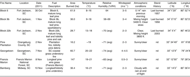
For each of the seven prescribed fires sampled in this study, the fuels, weather, size, lo-cation, etc. are shown in Table 1. The three prescribed fires of 30 October, 1 November, and 2 November 2011 (referred to as Blocks 6, 9b, and 22b, respectively) were located on the US Army’s Fort Jackson base northeast of Columbia, SC. Blocks 6, 9b, and
5
22b were last burned in 1957, 1956, and 2003, respectively. The overstory vegetation consisted primarily of mature southern pines, including longleaf pine and loblolly pine. High density pine areas had high canopy closure and limited understory vegetation with a thick litter layer (mostly pine needles). Lower density pine areas had turkey oak (Quercus laevis Walter) and other deciduous and herbaceous vegetation (i.e. grasses)
10
as significant components of the understory. Farkleberry (Vaccinium arboreum Marsh.), also known as sparkleberry, was present in significant quantities intermixed with ma-ture pine in Block 9b.
2.7 Airborne and ground-based sampling approach
The Fort Jackson prescribed burns (Blocks 6, 9b, and 22b) were part of a
collabora-15
tion with the forestry staff at the base. The LAFTIR ground-based sampling protocol was similar to that described in Burling et al. (2011). Background samples were ac-quired before the fire and the burns were ignited in the late morning or early after-noon. Ground-based sampling access was sometimes precluded during ignition, but sampling access then continued through late afternoon until each fire was effectively
20
out. During post-ignition access, numerous point sources of residual smoldering com-bustion (RSC) smoke were sampled by the mobile LAFTIR system minutes to hours after passage of a flame front. The spot sources of white smoke, mainly produced from pure smoldering combustion, included smoldering stumps, fallen logs, litter layers, etc., and they contributed to a dense smoke layer usually confined below the canopy. Point
25
ACPD
12, 25255–25328, 2012Reactive trace gases and O3 formation in
smoke
S. K. Akagi et al.
Title Page
Abstract Introduction
Conclusions References
Tables Figures
◭ ◮
◭ ◮
Back Close
Full Screen / Esc
Printer-friendly Version Interactive Discussion
Discussion
P
a
per
|
Dis
cussion
P
a
per
|
Discussion
P
a
per
|
Discussio
n
P
a
per
|
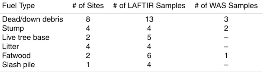
always collected prior to ignition as a background along with three sampled RSC point sources, also sampled by the LAFTIR system). Table 2 shows the RSC fuel types sam-pled on the ground for the Fort Jackson fires and Fig. 1 illustrates two of these fuels.
For the airborne measurements, mid-morning take-offs enabled us to sample the pre-fire background and then the initial emissions and adjacent backgrounds for as
5
long as the fire produced a convection column that exceeded several hundred meters in height. To measure the initial emissions from the fires, we sampled smoke less than several minutes old by penetrating the smoke column 150 to several thousand meters from the flame front. The goal was to sample smoke that had already cooled to the am-bient temperature since any chemical changes associated with smoke cooling are not
10
explicitly included in most atmospheric models. This approach also sampled smoke before most photochemical processing, which is explicitly included in most models. Afternoon flights were conducted to complete sampling of the initial emissions if nec-essary and to search for and sample the downwind plume (Figs. 2, 3, and 4). The plumes diluted rapidly mostly in the top half of a somewhat hazy boundary layer due
15
to variable winds (mixed layer extended to∼1100 m above mean sea level, a.m.s.l.). Thus, of the Fort Jackson fires, it was only possible to locate the downwind plume and obtain quality downwind data on the Block 9b fire (1 November, research flights number 3 and 4; RF03 and RF04 in Fig. 3, respectively). The prevailing winds on 1 November directed the plume through the Columbia metropolitan area and directly over an airport
20
and a natural gas power plant; thus mixing of burn smoke with fossil fuel emissions was unavoidable. The plume from the Block 22b fire directly entered a large restricted area and could not be subsequently re-sampled. However, while searching for the downwind plume we located a fire on a pine plantation about 40 km south of Columbia (Table 1). The Pine Plantation fire generated a Geostationary Satellite System (GOES) hotspot
25
ACPD
12, 25255–25328, 2012Reactive trace gases and O3 formation in
smoke
S. K. Akagi et al.
Title Page
Abstract Introduction
Conclusions References
Tables Figures
◭ ◮
◭ ◮
Back Close
Full Screen / Esc
Printer-friendly Version Interactive Discussion
Discussion
P
a
per
|
Dis
cussion
P
a
per
|
Discussion
P
a
per
|
Discussio
n
P
a
per
|
After the burns at Fort Jackson, we sampled additional fires throughout South Car-olina on 7, 8, and 10 November (Georgetown, Francis Marion, and Bamberg Fires, respectively). Due to transit time the Twin Otter typically arrived after the fire had been in progress for 0.5 to 1.0 h (ground-based sampling was not feasible due to long travel times and short notice). The airborne sampling of these fires initially focused on the
5
source emissions. After ∼1–1.5 h of repeatedly sampling the source, we would then cross the plume at increasingly large downwind distances until it could not be diff eren-tiated from background air. We then repeated the crossing pattern in reverse order or returned directly to the source approximately along the plume center-line depending on conditions (Fig. 4). The plumes from these three fires also diluted rapidly in the
bound-10
ary layer to form broad “cone-shaped” plumes under the influence of light and variable winds. Estimated times since emission, or smoke “ages”, were calculated for all the downwind samples by first calculating the average wind speed from the AIMMS-20 for incremental altitude bins of 100 m a.s.l. The smoke sample distance from the plume source was then divided by the average wind speed at the sample altitude, as shown
15
in Eq. (3). The majority of the uncertainty is in the wind speed variability, which was typically∼28 %.
Time Since Emission= Sample distance from source (m)
Wind speed (at sample altitude, m s−1) (3)
3 Results and discussion
3.1 Initial emissions
20
ACPD
12, 25255–25328, 2012Reactive trace gases and O3 formation in
smoke
S. K. Akagi et al.
Title Page
Abstract Introduction
Conclusions References
Tables Figures
◭ ◮
◭ ◮
Back Close
Full Screen / Esc
Printer-friendly Version Interactive Discussion
Discussion
P
a
per
|
Dis
cussion
P
a
per
|
Discussion
P
a
per
|
Discussio
n
P
a
per
|
strong correlation with CO as the reference species. However, the LAFTIR ground-based measurements showed greater scatter compared to airborne measurements, because the individual contributions from different fuel elements were measured sep-arately rather than blended together in a convection column (Bertschi et al., 2003). This increased scatter simply reflects real variability and not a decreased quality in the
5
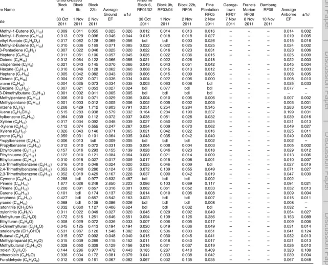
measurement of ERs. The fire-averaged and platform-based study average emission factors for all species measured are shown in Table 3. Measurements were obtained from both airborne and ground-based platforms for all Fort Jackson fires (Blocks 6, 9b, and 22b). Only airborne data were collected for the remaining four fires. WAS cans were collected for the Fort Jackson burns and the 2 November Pine Plantation burn.
10
Organic aerosol (OA) was measured by the AMS for five of the seven fires, and detailed AMS results will be presented in a complementary work (McMeeking et al., 2012). Up to 97 trace gas species were quantified by FTIR and WAS from both airborne and ground-based platforms, possibly the most comprehensive suite of trace gas species measured in the field for biomass burning fires to date.
15
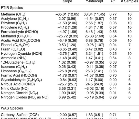
Emission factors for most species depend on the flaming to smoldering ratio, or MCE, and for this reason Table 4 shows linear regression statistics of EFs as a function of MCE for all fires sampled in this study. A negative slope denotes higher EF at lower MCE and that the compound is likely emitted by smoldering combustion (e.g. CH3OH). Conversely, a positive slope, indicating higher EF with increasing MCE, is normally
20
observed for compounds produced mainly by flaming combustion (e.g. NOx). Some species show poor correlation with MCE, indicating that other factors are dominating the variability in EF (e.g. phenol). Differences in fuel composition (e.g. %N) can also mask the dependence of EFs on MCE (Bertschi et al., 2003; Christian et al., 2007; McMeeking et al., 2009; Burling et al., 2010). Additionally, some compounds can be
25
ACPD
12, 25255–25328, 2012Reactive trace gases and O3 formation in
smoke
S. K. Akagi et al.
Title Page
Abstract Introduction
Conclusions References
Tables Figures
◭ ◮
◭ ◮
Back Close
Full Screen / Esc
Printer-friendly Version Interactive Discussion
Discussion
P
a
per
|
Dis
cussion
P
a
per
|
Discussion
P
a
per
|
Discussio
n
P
a
per
|
Numerous variables affect emissions and the predictive power of any one variable or small group of variables is limited.
3.2 Brief comparison to similar work
It is of interest to compare both the airborne and ground-based emission factors in this work to the EFs from the North Carolina coastal fires of Burling et al. (2011)
5
(Fig. 6). In the minimally-detailed global vegetation schemes in common use, both Burling et al. (2011) and this work measured EFs in temperate forest, and, more specif-ically, both studies measured EFs for prescribed fires burning in the understory of pine forests in the southeast US. However, there are some differences between the fires in our South Carolina (SC) study and the fires in North Carolina (NC) probed by Burling
10
et al. (2011). The NC fuels were comprised mostly of fine woody material and foliage, whereas our SC study included at least three fires where the fuels were mostly litter. In addition, the NC fire emissions were measured after an exceptionally wet spring, while the SC fires were sampled in the fall after a prolonged drought. Multiple factors likely contributed to the differences between these two studies (Korontzi et al., 2003) and the
15
effect of individual factors cannot be resolved from the available data. However, taken together, the two campaigns cover a more complete range of relevant environmen-tal and fuel conditions and provide a much-improved picture of the mean and natural variability for EFs for prescribed fires within a fairly narrowly defined ecosystem classi-fication. Our SC study-average MCE from airborne sampling was 0.931±0.016, which
20
is almost within 1−σstandard deviation of the average airborne MCE for the NC conifer forest understory burns (0.948±0.006). Of the 17 species (besides CO2and CO) mea-sured from the aircraft in both studies, only six compounds have EFs that agree within 35 %. We observed 52 % less NOxin SC, along with 22 and 33 % lower EF(HONO) and EF(NH3), respectively (Fig. 6a). The fuels burned in the NC fires likely included more
25
ACPD
12, 25255–25328, 2012Reactive trace gases and O3 formation in
smoke
S. K. Akagi et al.
Title Page
Abstract Introduction
Conclusions References
Tables Figures
◭ ◮
◭ ◮
Back Close
Full Screen / Esc
Printer-friendly Version Interactive Discussion
Discussion
P
a
per
|
Dis
cussion
P
a
per
|
Discussion
P
a
per
|
Discussio
n
P
a
per
|
(NMHCs) and oxygenated volatile organic compounds (OVOCs) were much higher in SC.
We can also compare the ground-based measurements from the two studies. Ground-based sampling of SC fires resulted in an MCE of 0.841±0.046, very similar to the 0.838±0.055 MCE measured in NC. EF(CO) and EF(CO2) agreed within 4 %, and
5
EF(CH4) agreed within 30 %. However, large differences were observed for most of the other 11 compounds measured in both studies. We report 73–97 % lower EFs in SC for all NMHCs that were measured in both studies (C2H2, C2H4, C3H6, 1,3-butadiene, and isoprene), which is the opposite of the EF(NMHC) comparison for the airborne mea-surements. We also observe 13–78 % higher EFs in the SC ground-based samples for
10
all the OVOCs measured in both studies (HCHO, CH3OH, CH3COOH, and C4H4O), which mimics the airborne comparison (Fig. 6b). The ground-based EF(NMHC) from SC, despite being lower than the ground-based EF(NMHC) in NC, are higher than all EF(NMHC) measured in laboratory burns of southeast pine litter (Burling et al., 2010). However, the MCE for the laboratory litter fires (0.894±0.017) was higher than both
15
the NC and SC ground-based MCEs. This brief overview makes it clear that large dif-ferences can be observed even in study-average emission factors for nominally similar ecosystems, most likely due in part to inherent large variability in the natural environ-ment: weather, fuels, etc.
3.3 Observation of large initial emissions of terpenes
20
3.3.1 Background levels and production in smoke plumes
Terpenes – hemiterpenes (isoprene), monoterpenes (C10H16), and sesquiterpenes (C15H24) – are emitted by plants in response to injury, disease, and other reasons (Paine et al., 1987; Guenther et al., 2006). Isoprene is synthesized by plants and then immediately emitted, but it is also a combustion product that is, for instance, emitted in
25
ACPD
12, 25255–25328, 2012Reactive trace gases and O3 formation in
smoke
S. K. Akagi et al.
Title Page
Abstract Introduction
Conclusions References
Tables Figures
◭ ◮
◭ ◮
Back Close
Full Screen / Esc
Printer-friendly Version Interactive Discussion
Discussion
P
a
per
|
Dis
cussion
P
a
per
|
Discussion
P
a
per
|
Discussio
n
P
a
per
|
are emitted immediately following synthesis, but the highest concentration of these compounds immediately adjacent to the plant is only a few ppb under normal conditions (Bouvier-Brown et al., 2009). However, very large concentrations of monoterpenes may be emitted into the gas phase (or “boiled off” via distillation) due to exposure to heat from fires (Simpson et al., 2011). Thus, the absolute mixing ratios of terpenes in
rela-5
tively undiluted fire emissions can exceed several ppmv and are much greater than the mixing ratios of these compounds from natural vegetative emissions.
3.3.2 High levels of terpenes in fresh smoke
The initial emissions of terpenes from biomass burning have been measured several times previously. Isoprene EF have been measured for some biomass fuels (Christian
10
et al., 2003; Yokelson et al., 2007a; Akagi et al., 2011; Simpson et al., 2011). Addition-ally, Yokelson et al. (1996) and Burling et al. (2011) noted large, IR spectral features in smoke similar to monoterpene absorption, suggesting possible large emissions of monoterpenes. Simpson et al. (2011) reported large EFs for two monoterpenes, α-pinene andβ-pinene, as measured by WAS from Canadian boreal forest fires during
15
the Artic Research of the Composition of the Troposphere from Aircraft and Satellites (ARCTAS) campaign. In this work we present the first quantitative FTIR observations of a monoterpene (limonene) in smoke along with an expanded suite of monoterpenes measured by WAS includingα-pinene,β-pinene, limonene, camphene, 4-carene, and myrcene – some for the first time from field fires. Our measured fire-averaged ERs
20
of these monoterpenes (and isoprene) from the ground-based and airborne platforms are shown in order of abundance in Table 5. In the SC smoke plumes, limonene and α-pinene are the most abundant monoterpenes measured from both the airborne and ground-based platforms, with limonene mixing ratios observed as high as 8.4 ppm.
Our study-averaged ER(∆α-pinene/∆CO) was more than 12 times higher in our
25
ACPD
12, 25255–25328, 2012Reactive trace gases and O3 formation in
smoke
S. K. Akagi et al.
Title Page
Abstract Introduction
Conclusions References
Tables Figures
◭ ◮
◭ ◮
Back Close
Full Screen / Esc
Printer-friendly Version Interactive Discussion
Discussion
P
a
per
|
Dis
cussion
P
a
per
|
Discussion
P
a
per
|
Discussio
n
P
a
per
|
a factor of 1.2 in the air (Table 5). Theα-pinene rate constants with respect to OH, O3, and NO3 are slower than those of limonene with these oxidants, suggesting that the much lowerα-pinene/limonene ratio in lofted smoke that reached the aircraft is not due to atmospheric oxidation. We suggest thatα-pinene may be preferentially released from fuels that burn largely by RSC (duff, dead-down woody fuels, etc.) and thus is
rela-5
tively more abundant in smoke that was poorly lofted in this study. The∆isoprene/∆CO ER was∼3.6 times greater in the lofted emissions sampled from the air, suggesting that RSC fuels may produce lower isoprene to CO ratios than the fuels that typically produce the bulk of lofted smoke (fine fuels, Akagi et al., 2011).
Figure 7 shows EFs (g kg−1) of monoterpenes and isoprene measured in this work.
10
In light of the above fuel-specific observations, it is of interest to further compare our terpene EFs with theα-pinene, β-pinene and isoprene EFs for boreal forest fires in Alberta, Canada measured by Simpson et al. (2011). Simpson et al. (2011) did not include limonene or other monoterpenes in their analysis due to the long analytical run-times required for the additional compounds. The sum of study-averaged α- and
15
β-pinene EFs from this work was 2.97±3.24 g kg−1 and 0.146±0.249 g kg−1 for the ground-based and airborne measurements, respectively. In comparison, the sum of α-and β-pinene EFs obtained during the airborne study of Simpson et al. (2011) had an intermediate value of 1.53±0.13 g kg−1and was obtained at an intermediate MCE of 0.90. Boreal forests often have a much greater loading of dead-down woody fuels
20
(due in part to slower decomposition) than temperate forests, and so relatively more of the emissions from these fuels may have been entrained in the lofted emissions sampled by Simpson et al. (2011). A higher contribution from the dead/down woody fuels would also be consistent with lower isoprene EFs of Simpson et al. (2011) (0.074± 0.017; Fig. 7). It should not be assumed, however, that unlofted smoke will always have
25
ACPD
12, 25255–25328, 2012Reactive trace gases and O3 formation in
smoke
S. K. Akagi et al.
Title Page
Abstract Introduction
Conclusions References
Tables Figures
◭ ◮
◭ ◮
Back Close
Full Screen / Esc
Printer-friendly Version Interactive Discussion
Discussion
P
a
per
|
Dis
cussion
P
a
per
|
Discussion
P
a
per
|
Discussio
n
P
a
per
|
levels of additional terpenes were also present in the ARCTAS samples that were not measured.
3.3.3 The influence of terpenes on smoke plume chemistry
We first assess the role of the dominant terpenes in daytime downwind VOC produc-tion in our biomass burning plumes. One important potential daytime oxidant – O3 –
5
was depleted in the freshest smoke via rapid reaction of background O3(∼50–80 ppb) with NO emitted by the fire (see Sect. 3.7 of this work; Yokelson et al., 2003b; Akagi et al., 2011, 2012). Thus, the reaction of limonene with OH would initially be the main daytime oxidation pathway forming low molecular weight products including methanol, formaldehyde, and acetone (Muller et al., 2005; Holzinger et al., 2005).α-Pinene, the
10
second most abundant monoterpene measured, reacts with OH to ultimately produce low molecular weight products such as acetone, formaldehyde, formic acid, and acetic acid (Capouet et al., 2004). Oxidation of terpenes via OH will be the main oxidation pathway for terpenes until O3 levels rebound in the plume, which can happen in as little as 0.5 h, at which time oxidation by both O3 and OH become important reaction
15
channels for the remaining terpenes. For limonene andα-pinene, we can estimate how long these species would remain in the plume given the elevated OH concentrations often found in biomass burning plumes (5×10⁶ to 1×10⁷molec cm−3, Hobbs et al., 2003; Yokelson et al., 2009; Akagi et al., 2012). Assuming a pseudo first-order decay of limonene andα-pinene with respect to OH (kOH+limonene=1.7×10⁻¹⁰cm3molec−1s−1,
20
kOH+α-pinene=5.3×10⁻¹¹cm3molec−1s−1; Bouvier-Brown et al., 2009) we estimate that
99 % of limonene and α-pinene will have reacted within 0.8–1.6 h and 2.5–4.9 h fol-lowing emission, respectively, with the higher [OH] estimate corresponding to faster monoterpene loss. As discussed later in Sect. 3.7, O3 can rebound to 80–100 ppb in as little as 1 h following emission (e.g. O3 levels can be well above background
25
ACPD
12, 25255–25328, 2012Reactive trace gases and O3 formation in
smoke
S. K. Akagi et al.
Title Page
Abstract Introduction
Conclusions References
Tables Figures
◭ ◮
◭ ◮
Back Close
Full Screen / Esc
Printer-friendly Version Interactive Discussion
Discussion
P
a
per
|
Dis
cussion
P
a
per
|
Discussion
P
a
per
|
Discussio
n
P
a
per
|
19–32 % and 9–16 % of the remaining limonene and α-pinene, respectively, would be due to oxidation via the O3 channel (kO3+limonene=2.0×10⁻¹⁶cm3molec−1s−1,
kO3+α-pinene=8.4×10⁻¹⁷cm3molec−1s−1; Bouvier-Brown et al., 2009), making
reac-tion with O3(and its byproducts) important though likely secondary to the OH reaction. Limonene reaction with O3has been shown to produce secondary photoproducts such
5
as formic and acetic acid, acetaldehyde, methanol, formaldehyde, and acetone (Lee et al., 2006; Walser et al., 2007; Pan et al., 2009) dependent on limonene and ozone levels. Recent work suggests the oxidation ofα-pinene with O3 produces low molec-ular weight byproducts including formaldehyde, acetaldehyde, formic acid, acetone, and acetic acid (Lee et al., 2006). Monoterpene ozonolysis also produces OH, with
10
OH molar yields of 0.86, 0.7–0.85, and 1.15 for limonene,α-pinene, and myrcene, re-spectively (Finlayson-Pitts and Pitts, 2000). Thus, reaction via the O3 channel would generate OH, increasing the oxidative capacity of the plume and encouraging further plume evolution. High levels of OH lead to increased O3formation which may help ex-plain the high O3formation rates observed during this campaign (Sect. 3.7). The small
15
molecule oxidation products of the other monoterpenes measured in this work (such asβ-pinene and myrcene) following oxidation by OH and O3are similar to those
prod-ucts already listed and include formaldehyde, formic and acetic acid, acetaldehyde, and acetone (Lee et al., 2006). Evidence of downwind growth in several of these VOCs has been previously observed in biomass burning plumes (Jost et al., 2003; Holzinger
20
et al., 2005; Karl et al., 2007; Akagi et al., 2011). While much effort has gone into un-derstanding and identifying monoterpene products, there is still considerable carbon mass tied up in unidentified species (Lee et al., 2006). In summary, since both the oxi-dant levels and the initial emissions of terpenes are highly variable in biomass burning plumes, we expect this to contribute to high variability in post-emission VOC production
25
as discussed in Sect. 3.7 and more generally in Akagi et al. (2011).
ACPD
12, 25255–25328, 2012Reactive trace gases and O3 formation in
smoke
S. K. Akagi et al.
Title Page
Abstract Introduction
Conclusions References
Tables Figures
◭ ◮
◭ ◮
Back Close
Full Screen / Esc
Printer-friendly Version Interactive Discussion
Discussion
P
a
per
|
Dis
cussion
P
a
per
|
Discussion
P
a
per
|
Discussio
n
P
a
per
|
smoldering or even flaming combustion that is perhaps promoted by nighttime frontal passage (Vermote et al., 2009; Turetsky et al., 2011). In this circumstance, some of the NOx may be tied up as NO3(Tereszchuk et al., 2011) promoting the reactions of terpenes and NO3, which produce formaldehyde, nitric acid (HNO3), and large organic nitrates and aldehydes, where the latter two products have oxidation products that are
5
not well studied (Fry et al., 2011). Assuming generic O3 and NO3 nighttime mixing ratios of 35 ppb and 5 ppt, respectively (Finlayson-Pitts and Pitts, 2000; Vrekoussis et al., 2004), about 90–91 % of the monoterpenes in smoke would react with NO3and the remainder mostly with O3. Production of alkyl nitrates from NO3 oxidation of fire-generated monoterpenes may tie up NOx for long-distance transport and may also
10
change the composition of secondary aerosol. In summary, most prescribed fires burn mostly during the day and most of the terpenes generated will be oxidized by OH. However, some fires produce smoke at night that probably has higher monoterpene content and most of those monoterpenes would be oxidized by NO3.
Considerable work has been done to investigate SOA yields from monoterpene
oxi-15
dation (Griffin et al., 1999; Spittler et al., 2006; Saathoffet al., 2009; Fry et al., 2011). While SOA formation via nucleation processes has been observed, the more common path for SOA formation occurs via condensation of gas-phase oxidation products onto pre-existing aerosol, given the ubiquitous presence of condensation surfaces in the at-mosphere (Hamilton et al., 2011). Limonene, the dominant monoterpene, is especially
20
susceptible to oxidation with two C=C double bonds (a.k.a. reactive sites, Fig. 7), pro-viding a quick, direct route to forming low-vapor pressure oxidation products that are likely to form a disproportionate amount of SOA relative to other monoterpenes (Lane et al., 2008; Maksymuik et al., 2009; Fry et al., 2011). In a biomass burning plume, extremely high amounts of NMOCs, and organic and inorganic aerosol are
simultane-25
ACPD
12, 25255–25328, 2012Reactive trace gases and O3 formation in
smoke
S. K. Akagi et al.
Title Page
Abstract Introduction
Conclusions References
Tables Figures
◭ ◮
◭ ◮
Back Close
Full Screen / Esc
Printer-friendly Version Interactive Discussion
Discussion
P
a
per
|
Dis
cussion
P
a
per
|
Discussion
P
a
per
|
Discussio
n
P
a
per
|
variables such as seed aerosol or oxidant concentration can be varied. Extrapolating chamber results to atmospheric conditions is not simple (Holzinger et al., 2010), but our confirmation of high levels of limonene and other terpenes in smoke plumes could help explain some of the variability in SOA production observed in fire smoke plumes to date (Saathoffet al., 2009; Hennigan et al., 2011; Akagi et al., 2012). It was
possi-5
ble to measure both the sum of monoterpenes by FTIR and/or WAS and the initial OA by AMS on three fires, which yielded mass ratios (Σmonoterpenes/OA g g−1) of 0.17, 0.15, and 0.36 (Table 3). The averageΣmonoterpenes/OA ratio measured in this work was 21 % on a mass basis and monoterpenes contributed to only 13.9 % of NMOC on a mass basis. Monoterpenes will not convert 100 % to SOA, and OA evolution in
10
biomass burning plumes may lead to small decreases in OA, or increases up to a fac-tor of∼3 (Hennigan et al., 2011). Thus, unless terpenes are emitted in much greater quantities from other fuel types they likely do not contribute to most of the total vari-ability observed in SOA. Because monoterpenes have 10 carbon atoms (Fig. 7), their oxidation could potentially contribute to a larger share of the variability observed in
pro-15
duction of smaller OVOCs downwind (Jacob et al., 2002; Jost et al., 2003; Holzinger et al., 2005, 2010; Yokelson et al., 2008, 2009; Pan et al., 2009; Akagi et al., 2012; Sect. 3.7).
3.4 C3−C4alkynes
A recent study was able to assign CO and other air-quality-relevant species observed
20
in the Mexico City area to either biomass burning or urban emissions by assuming that nearly all the HCN was emitted by biomass burning, while ethyne was emitted by both urban sources and fires, but with different ratios to CO (Crounse et al., 2009). Ethyne is emitted in higher proportion to CO by urban sources than by fires and the ethyne from biomass burning is usually produced mostly by flaming combustion (Lobert
25
ACPD
12, 25255–25328, 2012Reactive trace gases and O3 formation in
smoke
S. K. Akagi et al.
Title Page
Abstract Introduction
Conclusions References
Tables Figures
◭ ◮
◭ ◮
Back Close
Full Screen / Esc
Printer-friendly Version Interactive Discussion
Discussion
P
a
per
|
Dis
cussion
P
a
per
|
Discussion
P
a
per
|
Discussio
n
P
a
per
|
ideal tracer for any one source. Simpson et al. (2011) reported that other alkynes such as propyne have so far only been detected from biomass burning in widespread WAS measurements, making them of interest as possible biomass burning indicators despite having a relatively short lifetime of∼2 days. Our study-average ER(∆propyne/∆CO) of (4.51±0.50)×10−4 from the airborne-based platform is 2.5 times greater than the
5
ER(∆propyne/∆CO) reported by Simpson et al. (2011) (1.8±0.8×10⁻⁴) at a lower MCE suggesting more smoldering combustion in their study and that propyne may be emitted primarily by flaming combustion. We also observed the emission of higher alkynes (e.g. 1+2-butynes) from all the SC fires by WAS, which further suggests their potential use as biomass burning tracers. Finally, Fig. 8 shows that the three C3−C4
10
alkynes detected in this work are positively correlated with MCE and thus, like ethyne, are mostly produced by flaming combustion.
3.5 Initial emissions of nitrogen species
3.5.1 NH3
NH3is the most abundant alkaline gas in the atmosphere and is important in
neutraliz-15
ing acidic species in particulate matter (Seinfeld and Pandis, 1998). Biomass burning is an important NH3 source (Crutzen and Andreae, 1990) and biomass burning emis-sions of NH3 are typically strongly negatively correlated with MCE, meaning it is pri-marily emitted from smoldering combustion. We compare our EF(NH3) from both the air and ground with other EF(NH3) from biomass burning studies of similar fuel types
20
(Fig. 9). A general pattern emerges that the airborne EF(NH3) decrease going from California to Mexico to NC to SC and the ground-based EF(NH3) decrease from NC to SC. Thus, the SC EF(NH3) are systematically lower than observed in other studies of understory fires in pine-dominated forests. Other factors besides MCE can affect ammonia emissions, the most important being the nitrogen content of vegetation. The
25
ACPD
12, 25255–25328, 2012Reactive trace gases and O3 formation in
smoke
S. K. Akagi et al.
Title Page
Abstract Introduction
Conclusions References
Tables Figures
◭ ◮
◭ ◮
Back Close
Full Screen / Esc
Printer-friendly Version Interactive Discussion
Discussion
P
a
per
|
Dis
cussion
P
a
per
|
Discussion
P
a
per
|
Discussio
n
P
a
per
|
work is unknown, this could explain why the ground-based samples (often of smol-dering logs/stumps) had EF(NH3) that were generally lower than the airborne data regression relationship would predict.
3.5.2 HCN
HCN is produced from the pyrolysis of amino acids and is now widely recognized as
5
a useful biomass burning tracer (Li et al., 2003; Crounse et al., 2009). We compare the ER(∆HCN/∆CO) from this work to other works in similar fuels, including pine-forest understory burns (Burling et al., 2011), Mexican rural pine-oak pine-forests (Yokelson et al., 2011), Canadian boreal forests (Simpson et al., 2011), and US pine litter from Georgia (Burling et al., 2010) (Fig. 10). We also include ERs from some very different,
10
but globally important fuel types, including savanna fires from Africa (Yokelson et al., 2003b), tropical evergreen deforestation fires from Brazil (Yokelson et al., 2007a), peat-land (Akagi et al., 2011), and fires in tropical dry forest (Yokelson et al., 2009). The study means for the airborne measurements of ER(∆HCN/∆CO) shown in Fig. 10 all fall within the range 0.0063 to 0.0095. The ground-based and lab measurements are
15
lower than this range with the exception of the ER(∆HCN/∆CO) from peatland fires, which, at 0.03±0.036, is more than three times larger than the other values (Akagi et al., 2011). In both this work and Burling et al. (2011), lower HCN emission ratios are observed from a ground-based versus airborne platform when sampling the same fires.
20
Overall, the airborne and ground-based EF(HCN) show a strong negative correlation with MCE suggesting that HCN is released from smoldering combustion over a wide range of MCEs (0.85–0.96) (Fig. 11). This high negative correlation is seen in results from pine-forest organic soils collected from Montana, US and the Northwest Territo-ries, Canada (Bertschi et al., 2003). By contrast, airborne EF(HCN) measured in some
25
ACPD
12, 25255–25328, 2012Reactive trace gases and O3 formation in
smoke
S. K. Akagi et al.
Title Page
Abstract Introduction
Conclusions References
Tables Figures
◭ ◮
◭ ◮
Back Close
Full Screen / Esc
Printer-friendly Version Interactive Discussion
Discussion
P
a
per
|
Dis
cussion
P
a
per
|
Discussion
P
a
per
|
Discussio
n
P
a
per
|
The similarity of study-averaged ERs shown in Fig. 10 and the observation that fire-averaged MCE usually fall in the range of 0.90–0.94 (Fig. 11) confirm that HCN is a useful tracer for the lofted emissions that account for much of the smoke generated by many fires around the world. However, the larger scatter at low MCE in Fig. 11 suggests that HCN may be a better tracer for smoke that is lofted and transported as
5
opposed to smoke that drifts at ground level. Finally, the variability in HCN emissions is magnified when considering a broader range of fuel types. For instance, there are very large EF(HCN) emissions from peat, while Christian et al. (2010) report that HCN was below FTIR detection limits when sampling cooking fire emissions in both Mexico and Africa.
10
3.5.3 Nitrous acid (HONO)
HONO is an important precursor for OH radicals in the atmosphere (Broske et al., 2003). Photolysis is the primary daytime fate of HONO and it forms OH and NO within 10–20 min (Schiller et al., 2001). Given the importance of OH as a key atmospheric oxidant, photolysis of HONO could significantly affect the photochemistry of some
ag-15
ing plumes (Alvarado and Prinn, 2009). HONO is now recognized as a major flaming combustion product from fires that has been measured in both lab and field experi-ments (Trentmann et al., 2005; Keene et al., 2006; Yokelson et al., 2007a, 2009; Burl-ing et al., 2010; 2011). In SC, HONO was detected by AFTIR durBurl-ing four of the seven fires. The measureable ∆HONO/∆NOx molar ratios ranged from 0.158 to 0.329 with
20