Experimental investigations and validation of a new material model developed for masonry bricks

ESCOLA DE ENGENHARIA

PROGRAMA DE PÓS-GRADUAÇÃO

EM ENGENHARIA DE ESTRUTURAS

EXPERIMENTAL INVESTIGATIONS AND

VALIDATION OF A NEW MATERIAL MODEL

DEVELOPED FOR MASONRY BRICKS

I would first like to thank the Department of Structural Engineering from the UFMG (Federal University of Minas Gerais) for the trust in my work. In particular, my greatest thanks go to my supervisor Prof. Roberto Márcio da Silva. Thanks for the great amount of e-mails and meetings with rich discussions and ideas.

More than special thanks go to my supervisor at the UniBw (University of the Bundeswehr), Prof. Norbert Gebbeken, and my colleagues who shared very rich ideas that helped to make this work.

Also many thanks go to Dr. Andrea Kustermann and her team at the UniBw for executing the material tests with bricks.

And finally my eternal thanks go to my family, my fiancé Franz Engel, and friends for the emotional support.

Tamara Vieira Araújo

This Master Thesis presents static and dynamic material tests conducted for different types of bricks and numerical simulations developed to model static tensile and compression tests conducted at the University of the Bundeswehr. Based on the results of the experimental investigations, a new material model for masonry bricks was developed. This model was implemented with a user subroutine developed in ANSYS AUTODYN. These material models, which are suitable for a detailed micro-model approach, consider the dynamic increase of the material strength and the degradation of the material properties due to fracture and material damage. In this Master Thesis, the analysis of the experimental investigations, the material model developed for bricks and its verification and validation for static tensile and compressive tests are presented.

Keywords: Masonry, bricks, detailed micro-model, experimental investigations, static and

Esta dissertação de Mestrado apresenta ensaios experimentais estáticos e dinâmicos de materiais realizados para diferentes tipos de tijolos e simulações numéricas desenvolvidas para modelar os ensaios estáticos de tração e compressão conduzidos na Universidade das Forças Armadas Alemãs. Com base nos resultados dos ensaios, um novo modelo de material para tijolos maciços de alvenaria foi desenvolvido. Este modelo foi implementado através de uma subrotina desenvolvida no programa ANSYS AUTODYN. O modelo constitutivo foi baseado na estratégia de micro-modelagem detalhada, e considera o aumento da resistência do material devido à ações dinâmicas e a degradação do material devido à falhas e danos. Nesta dissertação de Mestrado, a análise dos ensaios, o modelo de material desenvolvido para tijolos maciços de alvenaria e a verificação e validação dos ensaios estáticos de tração e de compressão serão apresentados.

Palavras-chave: Alvenaria, tijolos maciços, micro-modelagem detalhada, ensaios, modelo

ABSTRACT ... v

RESUMO ... vii

LISTOFFIGURES ... xi

LISTOFTABLES ... xv

LISTOFSYMBOLS ... xvii

1 INTRODUCTION ... 1

1.1 Problem characterization ... 5

1.2 Objective ... 6

1.3 Methodology ... 6

1.4 Master Thesis structure ... 8

2 MATERIAL PROPERTIES OF THE BRICKS ... 9

2.1 Static tensile tests on bricks ... 10

2.1.1 Uniaxial tensile tests ... 11

2.1.2 Brazilian splitting tests (indirect tensile test) ... 21

2.2 Static compression tests on bricks ... 24

2.3 Dynamic tensile and compression tests of bricks ... 32

3 MATERIAL MODEL FOR BRICKS... 43

3.1 Definition of stress invariants ... 43

3.2 Strength model ... 49

3.3 Tension cut-off with Rankine criterion ... 52

3.4 Elastic and plastic material status, residual strength and damaged material status ... 53

3.5 Adaption of the material stiffness ... 58

3.6 Adaption of Young’s Moduli, tensile and compression regime ... 59

3.7 Strain rate dependency... 59

3.8 Equation of state ... 62

4 NUMERICAL SIMULATIONS ... 65

4.1 Hydrocode simulations ... 65

4.2 Verification of the brick material model ... 68

4.3 Validation of the brick material model ... 74

5 CONCLUSION ... 77

5.1 Suggestions for future work ... 78

6 REFERENCES ... 81

A APPENDIX ... 87

A.1.2 Clinker brick ... 90

A.1.3 Clay brick (Germany) ... 93

A.1.4 Clay brick (Afghanistan) ... 96

A.1.5 Concrete brick ... 99

A.2 Compressive tests ... 102

A.2.1 Ceramic brick... 102

A.2.2 Clinker brick ... 104

A.2.3 Clay brick (Germany) ... 106

A.2.4 Clay brick (Afghanistan) ... 108

Figure 1.1 - Masonry wall with its components, ceramic bricks and cement mortar ... 1

Figure 1.2 - Definition of the brick faces ... 2

Figure 1.3 - Masonry bonds with courses of mixed headers and stretchers ... 2

Figure 1.4 - Masonry bonds with one stretcher course per header course ... 2

Figure 1.5 - Masonry bonds with more than one stretcher course per header course ... 2

Figure 1.6 - Masonry bonds with only stretcher courses or only header courses ... 3

Figure 1.7 - Masonry bonds with courses of mixed stretchers and soldiers ... 3

Figure 1.8 - Masonry bonds with courses of mixed rowlocks and shiners ... 3

Figure 1.9 - Masonry bonds build around square fractional-sized bricks ... 3

Figure 1.10 - Strategies to model masonry numerically ... 4

Figure 1.11 - Examined bricks (left to right): clinker, ceramic, German clay, Afghan clay and concrete ... 7

Figure 2.1 - Schematic of the stress components in a masonry specimen during a compression test (left) based on Bierwirth (1994), and response of a masonry specimen after a uniform uniaxial compressive stress (right) ... 10

Figure 2.2 - Universal test machine at the UniBw used for the tensile tests ... 11

Figure 2.3 - Ceramic brick with notches in the middle (left) and bricks after the tensile test (right) ... 12

Figure 2.4 - Force-displacement curve obtained from the tensile test for the ceramic brick with notches (force-controlled)... 13

Figure 2.5 - Inductive transducers implanted in the bricks, ceramic brick ... 17

Figure 2.6 - Tensile stress-strain curve obtained from the tensile test for the determination of a ceramic brick (VZ1) E-Modulus and points used for the determination of the E-Modulus of concrete according to the German (DIN 1045) and Brazilian (NBR 8522) norms ... 19

Figure 2.7 - Clay brick (Afghanistan), ceramic and clinker brick (Germany), left to right ... 21

Figure 2.8 - Preparation of the ceramic brick geometry, cutting in cylindrical form (left) and cutting the body for the specified height (right) ... 22

Figure 2.9 - Polishing the bottom and top faces (left) and cylindrical ceramic specimen after polishing (right) ... 22

Figure 2.10 - Brazilian splitting test, sketch (left) and real test with ceramic brick (right) ... 23

Figure 2.11- Compression tests with different geometries, standing Afghan clay (left), lying ceramic brick (right) and cylindrical ceramic brick (middle) (force-controlled) ... 25

Figure 2.14 - Compressive stress-strain curve obtained from the compressive test for the

determination of one of the ceramic brick E-Modulus ... 29

Figure 2.15 - Approximated correlation interpreted from Ngo et al. (2007), Linse (2012) and Ramesh (2008) ... 32

Figure 2.16 - Basic operation system of Split-Hopkinson-Bar ... 33

Figure 2.17 - Used impact system for the Split-Hopkinson-Bar ... 33

Figure 2.18 - Crack propagation during indirect dynamic tensile test, Brazilian test ... 34

Figure 2.19 – Dynamic compression test conducted in Split-Hopkinson-Bars ... 34

Figure 2.20 - Incident strain ( e), reflected strain ( r), transmitted strain ( t) and displacements (u1 and u2) during a SHB test in a specimen of length Ls ... 35

Figure 2.21 - Dynamic increase factors for the tensile strength of concrete specimens (black symbols), Schuler et al. (2006), and own tests results for bricks ... 40

Figure 2.22 - Dynamic increase factors for the compressive strength of concrete specimens (black symbols), Bischoff and Perry (1995), and own tests results for bricks ... 40

Figure 3.1 - Sketch from a material stress state under triaxial tensile stress (left) and under triaxial compressive stress (right) ... 44

Figure 3.2 - Projection on the deviatoric plane of the coordinate’s axis σ1, σ2and σ3 (left) and stress decomposition in the principal stress space (right)... 48

Figure 3.3 - Representation of the material test position on the stress surface, Linse et al. (2012) ... 50

Figure 3.4 - Schematic representation of the material status, the fracture strains, the residual strength and the strain when residual strength is achieved, Gebbeken et al. (2011) ... 54

Figure 3.5 - Effective fracture strain as a function of triaxiality ( ), Gebbeken et al. (2011) .. 55

Figure 3.6 - Residual strength as a function of the triaxiality of the stress state, Gebbeken et al. (2011) ... 57

Figure 3.7 - Adaption of the fracture surface due to material damage for several stress states, Gebbeken et al. (2011)... 58

Figure 3.8 - Proposed dynamic increase factor curve for the tensile strength of concrete specimens, red curve, Hartmann et al. (2010) and for bricks, blue curve, Linse (2012)... 60

Figure 3.9 - Proposed dynamic increase factor curve for the compressive strength of concrete specimens, red curve, Hartmann et al. (2010) and for bricks, blue curve, Linse (2012)... 61

Figure 3.10 - Schematic porous equation of state for concrete (Hartmann (2009)) ... 63

Table 1.1 - Sizes and densities of the examined bricks ... 7

Table 2.1 - Tensile strength (ft) obtained for the ceramic brick ... 15

Table 2.2 - Grubb numbers obtained for the ceramic brick ... 16

Table 2.3 - Ceramic brick E-Modulus obtained from different norms ... 20

Table 2.4 - E-Moduli obtained for the masonry bricks under tensile stress (DIN 1045) ... 20

Table 2.5 - Indirect tensile strength obtained for the masonry bricks cylindrical specimens from the Brazilian splitting tests ... 24

Table 2.6 - Compressive strength (fc) obtained for the ceramic bricks ... 27

Table 2.7 - E-Moduli obtained for the masonry bricks under compressive stress ... 29

Table 2.8 - Compressive strength obtained for the masonry bricks cylindrical and cubic specimens from the compression tests... 31

Table 2.9 - Dynamic tensile strength (fst, dyn) obtained for bricks ... 37

Table 2.10 - Dynamic compressive strength (fc, dyn) obtained for bricks ... 38

Table 2.11 - Dynamic Increase Factor (DIF) obtained for the bricks ... 39

Table 3.1 - Material parameters for masonry units, Linse (2012) ... 52

Table 3.2 - Residual strength for different stress states, based on Bierwirth’s material tests .. 56

Table 3.3 - Fracture strains for masonry bricks ... 57

Table 4.1 - Stresses and strains of the numerical simulations and theoretical values ... 71

Table 5.1 - E-Moduli obtained for the bricks under tensile and compressive stresses ... 78

Table A.1 - Tensile strength (ft) obtained for the ceramic bricks ... 88

Table A.2 - Tensile strength (ft) obtained for the clinker bricks ... 91

Table A.3 - Tensile strength (ft) obtained for the German clay bricks ... 94

Table A.4 - Tensile strength (ft) obtained for the Afghan clay bricks ... 97

Table A.5 - Tensile strength (ft) obtained for the concrete bricks ... 100

Table A.6 - Compressive strength (fc) obtained for the ceramic bricks ... 103

Table A.7 - Compressive strength (fc) obtained for the clinker bricks ... 105

Table A.8 - Compressive strength (fc) obtained for the German clay bricks ... 107

Table A.9 - Compressive strength (fc) obtained for the Afghan clay bricks ... 109

Small Latin letters

a element accelerations c wave propagation speed cv coefficient of variation

d diameter of the specimen e internal energy

fc, fc,stat static compressive strength

fc, dyn dynamic compressive strength

fct uniaxial tensile strength for Ottosen’s criteria

fcc biaxial compressive strength for Ottosen’s criteria

f2c relation between the biaxial and uniaxial compressive strength for Ottosen’s criteria

ft, ft, stat static tensile strength

ft, dyn dynamic tensile strength

fst indirect static tensile strength

fst, dyn indirect dynamic tensile strength

f stability time step factor h length of the specimen

k relation between the uniaxial tensile and compressive strength for the Ottosen’s criteria

k1, k2 parameters for the Ottosen’s criteria

m element mass p hydrostatic pressure s standard deviation

Δt time step

u1 deformation at the initial of the specimen

u2 deformation at the end of the specimen

A cross sectional area between the notches Ai initial cross sectional area

Cor correction factor

D damage

DIF dynamic increase factor F applied force

Fmax maximum applied force

G gain

Gbrick brick shear modulus

G0 undamaged shear modulus

I1 first invariant of the stress tensor σij

I2 second invariant of the stress tensor σij

I3 third invariant of the stress tensor σij

J1 first invariant of the deviatoric stress tensor sij

J2 second invariant of the deviatoric stress tensor sij

J3 third invariant of the deviatoric stress tensor sij

K sensibility factor L final length

ΔL variation of the elongation

Li initial length considered to measure the elongation

N number of samples R residual strength T stress tensor

U0 corrected measured voltage

U1 applied electric voltage

Greek letters

Kronecker delta engineering strain Δ variation of strain

e incident strain r reflected strain t transmitted strain ̇s strain rate

eff,B, 1Z fracture strain obtained from the uniaxial tensile test eff,B, 1D fracture strain obtained from the uniaxial compressive test eff,B, 3D fracture strain obtained from the triaxial compressive test

eff,R residual strength

λ function for the Ottosen’s criteria

B,1Z triaxiality by fracture from the uniaxial tensile test B,1D triaxiality by fracture from the uniaxial compressive test B,3D triaxiality by fracture from the triaxial compressive test

Poisson’s ratio

ϴ element temperature

hydrostatic axes in the Haigh-Westergaard stress space ρ deviatoric axes in the Haigh-Westergaard stress space

engineering stress Δ variation of stress

max maximum obtained stress a minimum obtained stress b one third of σmax

z axial stress r, radial stress ii principal stresses

m mean stress or hydrostatic stress oct octahedral normal stress

o octahedral normal stress for Ottosen’s criteria

shear stress

oct octahedral shear stress

o octahedral shear stress for Ottosen’s criteria

1

1

I

NTRODUCTION

Masonry is one of the most important construction materials used for buildings worldwide. A masonry wall is composed of masonry bricks and mortar (Figure 1.1), in which the bricks are joined together by the mortar. A wide range of materials for masonry bricks and for mortar is used in practice. The bricks can be made of several materials such as concrete, ceramic, stone, clay or glass; and the mortar can be made of materials such as cement, clay, lime or sand.

Figure 1.1 - Masonry wall with its components, ceramic bricks and cement mortar

Figure 1.2 - Definition of the brick faces

Flemish bond Monk bond Raking monk bond

Flemish garden wall bond Flemish diagonal bond Figure 1.3 - Masonry bonds with courses of mixed headers and stretchers

English bond English cross bond Double English cross bond Figure 1.4 - Masonry bonds with one stretcher course per header course

English garden wall bond Scottish bond American bond

Stretcher bond Raking stretcher bond Header bond Figure 1.6 - Masonry bonds with only stretcher courses or only header courses

Single basket weave bond Double basket weave bond

90° Herringbone bond 45° Herringbone bond

Figure 1.7 - Masonry bonds with courses of mixed stretchers and soldiers

Rap-trap bond

Figure 1.8 - Masonry bonds with courses of mixed rowlocks and shiners

Pinwheel bond Della robia bond

Figure 1.9 - Masonry bonds build around square fractional-sized bricks

Nowadays, along with the software development, a physical structure can be modeled as often as necessary without having to build it physically. This means lower research costs compared to previous times. However, most structures are not so simple to model numerically. In the numerical analyses of masonry, the different materials, the different sizes of the bricks and the different possibilities to assemble the bricks must also be considered.

In the 70s, an Australian researcher (Page (1978)), considered masonry as a two-phase material consisting of elastic materials, the bricks, placed into an inelastic mortar matrix. He characterized the masonry in this way because he considered that most of the inelastic deformation occurred in the joints, and the joint characteristics were affected by the magnitude of the shear and normal stresses in the joint.

According to Page (1978), assumptions of isotropic elastic behavior could be satisfactory in predicting deformations at low stress levels in the working range. However, they are not expected to be adequate at higher stress levels when extensive stress redistribution will occur. This redistribution is caused by non-linear material behavior (predominantly in the mortar joints), and failure in localized areas due to loss of bond between mortar and brick.

This was a short description about the earliest forms of mechanical characterization of the masonry walls. Nowadays, there are several strategies to model masonry walls numerically (Figure 1.10). These strategies can be classified into two main groups: micro-models and macro-model. Micro-models are usually distinguished between detailed and simplified micro-models. In the following, a brief description of each method is presented.

In the first case, detailed micro-model, the bricks and the mortar joints have their real sizes. Bricks and mortar are modeled as continuum elements. Using the detailed micro-model, the

Young’s modulus (E-Modulus), the lateral deformation (Poisson’s ratio) and the inelastic material properties of the mortar and the bricks can be modeled separately. This is important in order to assess the failure due to lateral tension in the bricks. Therefore, the interaction between the mortar and the bricks and the different failure modes can be realistically determined.

In the second case, simplified micro-model, the mortar joints are numerically described by interface elements, which represent the material properties of the mortar. At the same time, they describe the properties of the transition zone and the bond between brick and mortar. The interface elements usually do not have a thickness. Therefore, the sizes of the masonry units have to be adapted. In order to model the properties of the mortar joints and the bond between mortar and brick, non-linear spring elements can be used in order to consider material models.

In the third case, macro-models, the inhomogeneous composite material of masonry, composed of the two materials, mortar and bricks, are numerically replaced by one homogeneous material. This means that the properties of the brick, the mortar and the transition zone between mortar and brick are homogenized and described by one material model. As a consequence, some information about the individual constituents can be lost. However, the macro-models are often used to model entire masonry structures because it is possible to obtain results faster.

1.1 Problem characterization

Due to the extensive use of masonry around the world, it is necessary to better study the

behavior of the material’s components subjected to different actions.

(Non-Governmental Organizations), as well as military camps and historical buildings have become targets for these high dynamic actions.

This means that besides the need to understand the behavior of masonry constructions subjected to static actions, nowadays a better protection and a better assessment of buildings against high dynamic actions are needed. These exceptional actions show the importance to develop models to better describe the mechanical behavior of the masonry walls.

1.2 Objective

Studies with the first strategy explained before, a detailed micro-model, were developed at the University of the Bundeswehr (UniBw - Universität der Bundeswehr München), Linse (2012). Two material models were developed, one for the mortar and one for the bricks.

The main objective of this work is to verify and validate the material model developed for bricks.

In order to achieve this objective, the following main points described in the methodology have to be developed and studied.

1.3 Methodology

Figure 1.11 - Examined bricks (left to right): clinker, ceramic, German clay, Afghan clay and concrete

Table 1.1 - Sizes and densities of the examined bricks

Brick Sizes [mm] Density [g/dm³]

Clinker 237x110x71 2143 Ceramic 239x115x72 1807 German clay 247x118x66 1139 Afghan clay 207x100x74 1497 Concrete 241x114x114 1899

1.3.1 Analysis of the experimental investigations

In order to obtain the mechanical properties of the bricks, several static and dynamic experimental investigations were conducted with five types of bricks. Static tensile, compression and Brazilian tests were carried out at the UniBw.

In addition, dynamic Split-Hopkinson-Bar tests were carried out at the Joint Research Centre (JRC) of the European Commission, in Ispra, Italy.

The results of all experiments are going to be analyzed.

1.3.2 Verification and validation of the material model developed for bricks

In order to verify the material model, the tensile and compression static tests were numerically simulated and the results were compared with the continuum theory.

Also the results obtained in the simulations were validated with the results obtained in the experimental investigations. The comparisons between the numerical results and those of the tensile and compression static tests will be presented.

1.4 Master Thesis structure

The structure of this Master Thesis consists of the following chapters:

 chapter 2- material properties of the bricks: in this chapter the material properties of the bricks obtained from experimental investigations will be described. Tests were conducted with different loadings being static or dynamic. Static tensile and compressive tests were conducted at the University of the Bundeswehr (UniBw) and dynamic Split-Hopkinson-Bar tests were developed at the Joint Research Centre (JRC).

 chapter 3- material model for bricks: in this chapter the material model developed for bricks with its mechanical characteristics will be described. The material model is a new propose developed at the masonry group at the UniBw;

 chapter 4- numerical simulations: in this chapter the numerical simulations developed in ANSYS AUTODYN for the tensile and compressive static tests conducted at the UniBw will be presented. Moreover the verification and validation of the material model will be presented;

2

2

M

ATERIAL

P

ROPERTIES OF THE

B

RICKS

Although there is experimental test data of masonry specimens existing, there is little data available for the masonry components, bricks and mortar. Often, tests are performed on masonry specimens in order to determine the maximum bearing capacity. However, the properties of the components are neither reported nor tested at all. Nevertheless, there are some publications that deliver detailed information on bricks. Vermeltfoort and Pluijm (1991) and Pluijm (1992) carried out tests in order to determine the tensile strength of mortar joints, the compressive and tensile strength of different types of bricks, and the Young’s Moduli for both materials. Sarangapani et al. (2005) studied the bond between brick and mortar and published data for Indian mortar and bricks. Schubert (2005), Schubert (2007) and Brameshuber et al. (2006) assembled further data, especially for typical German masonry materials.

The masonry bricks can be made of different materials, e.g., adobe, clay, ceramic, clinker, concrete or calcium silicate. Consequently, the uniaxial compressive strength of masonry units, for example, can range from 3 to 100 MPa. In addition, the number of highly sophisticated masonry units with voids and internal thermal insulation is increasing, which have different mechanical properties compared to solid bricks.

2.1 Static tensile tests on bricks

An important material parameter for bricks is the tensile strength because bricks usually fail under tensile stresses and strains without significant deformation. Even if there is a uniform compressive stress in the plane of a masonry wall, besides lateral tension due to the Poisson’s effect, lateral tension is introduced in the bricks due to the mortar. Figure 2.1 shows schematically the stresses in the masonry components and the response of a masonry specimen after a uniform uniaxial compression test. It is possible to see that the bricks fail due to tensile stress even though a compressive stress is applied.

Figure 2.1 - Schematic of the stress components in a masonry specimen during a compression test (left) based on Bierwirth (1994), and response of a masonry specimen after a uniform

uniaxial compressive stress (right)

2.1.1 Uniaxial tensile tests

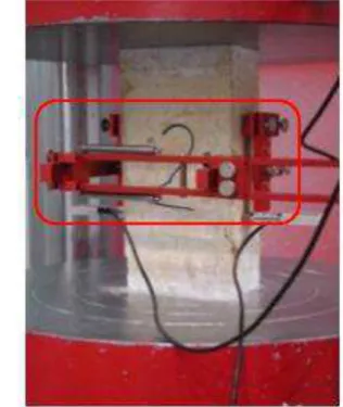
The tensile tests were conducted in a universal test machine (Figure 2.2). The specimens were embedded with epoxy glue in the grips and due to the moveable crosshead, the load was applied and recorded, and the displacement of the moveable crosshead could be obtained.

Figure 2.2 - Universal test machine at the UniBw used for the tensile tests

There are two methods to run the tests, path-controlled or force-controlled. In the case of path-controlled the moveable crosshead is programmed to run until a specified maximum displacement; and in the case of force-controlled, the moveable crosshead is programmed to apply a force until a maximum specified force. Then the probe is subjected to uniaxial tension, if the moveable crosshead is running to stretch the specimen until failure; or compression, if the moveable crosshead is running in order to compress the specimen until failure.

curve can be obtained. Unlike the path-controlled, the force-controlled does not move along the yield curve and can therefore only be used for determining the stable path until failure on the yield curve.

The tensile tests were force-controlled, and in order to observe the influence of the velocity in which the force was applied, three different velocities were used.

Small cracks can exist along the specimen and probably the brick will fail in the region of these small cracks, which exist because of the drying and burning process of the bricks. In order to obtain the tensile strength of the material, possibly without the influence of the brick cracks, two lateral notches were cut, with a diamond sawing machine, in the middle of the five different bricks (Figure 2.3). The idea behind conducting these tests was to obtain the tensile strength in a very small specific region in the middle of the brick. Figure 2.3 shows the ceramic brick specimen with the notches in the middle and the considered areas for the determination of the tensile strength.

Figure 2.3 - Ceramic brick with notches in the middle (left) and bricks after the tensile test (right)

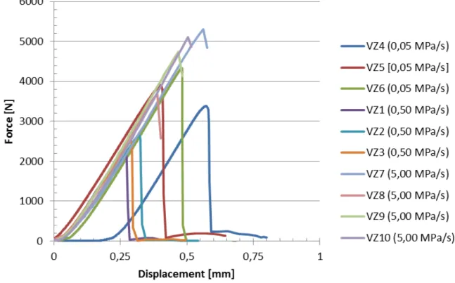
and VZ3 fail at a lower applied force. This happens because these specimens have a small cross sectional area between the notches.

Figure 2.4 - Force-displacement curve obtained from the tensile test for the ceramic brick with notches (force-controlled)

The tensile strength (ft) can then be obtained with Equation (2.1).

[ ] _[ [ ]_] (2.1)

where Fmax is the maximum applied force;

A is the cross sectional area between the notches.

In addition, in order to measure the dispersion between the obtained tensile strength and the average of the test results, the Standard deviation (s) was obtained using Equation (2.2).

√ _∑ ̅

where N is the number of samples; xi is the obtained test result; ̅i is the average of the test results.

If the measured dispersion is low, it means that the test results tend to be very close to the mean, and this situation is always expected. However, if the measured dispersion is high, it means that the test results are not so close together and in some cases it would be recommended to do more tests in order to obtain a low dispersion.

With the coefficient of variation (cv), the percentage ratio between the standard deviation and

the average can be obtained (Equation (2.3)).

(2.3) where σ is the standard deviation;

μ is the average value obtained from the results.

Table 2.1 - Tensile strength (ft) obtained for the ceramic brick

Specimen Fmax [N] Area [mm²] Tensile strength [MPa]

VZ4 3380,50 130 0,81 VZ5 3903,60 130 0,93 VZ6 4331,75 131 1,02 VZ1 2278,45 101 1,07 VZ2 2656,65 101 1,25 VZ3 2510,40 101 1,18 VZ7 5310,35 130 1,27 VZ8 3678,15 130 0,88 VZ9 4746,55 131 1,11 VZ10 5101,85 121 1,46

Average tensile strength 1,10

Standard deviation (s) 0,20

Coefficient of variation (cv) 18,18%

In order to know if there are values that should be discarded, the Grubbs test was conducted. The test compares the outlying data points with the average and standard deviation (Equation .

| ̅| (2.4)

where G is the Grubb number; xi is the obtained test result; ̅i is the average of the test results;

σ is the standard deviation.

Table 2.2 - Grubb numbers obtained for the ceramic brick

x ̅i G

0,81 1,1 0,2 1,45 0,93 1,1 0,2 0,85 1,02 1,1 0,2 0,40 1,07 1,1 0,2 0,15 1,25 1,1 0,2 0,75 1,18 1,1 0,2 0,40 1,27 1,1 0,2 0,85 0,88 1,1 0,2 1,10 1,11 1,1 0,2 0,05 1,46 1,1 0,2 1,80

Based on a comparison with a tabulated criterion that depends on the number of test results, the point is either validated or discarded as being statistically irrelevant. According to this table if the number of samples is 11, the tabulated criterion is 2,234. The Grubb numbers obtained are lower than 2,234, that means that none of the test results should be discarded.

Figure 2.5 - Inductive transducers implanted in the bricks, ceramic brick

With this obtained elongation from the inductive transducers, it is possible to calculate the engineering strain ( ) (Equation. (2.5)):

(2.5)

where ∆L is the variation of the length,

Li is the initial length considered to measure the elongation, 10 mm (Figure 2.5),

L is the final length.

The engineering stress (σ) is obtained using Equation (2.6):

(2.6)

where F is the applied force,

Applying Hooke’s Law (Equation (2.7)), the E-Modulus (E) can be obtained:

(2.7)

where Δσ is the variation of the stress,

Δ is the variation of the strain.

There isn’t any norm for the determination of brick E-Modulus. And in this way the procedure described in the German norm (DIN 1045) for the determination of the concrete E-Modulus was adopted.

The procedure described in the Brazilian norm for the determination of the concrete E-Modulus was also analyzed. The results obtained with the German norm (DIN 1045) were compared with the results obtained with the Brazilian norm (NBR 8522) procedure.

According to the German Norm, Equation (2.8) should be considered.

(2.8)

where σmax is the maximum obtained stress; max is the maximum obtained strain.

On the other hand, according to the Brazilian Norm, Equation (2.9) should be used to the determination of the E-Modulus of concrete:

(2.9)

where σbis a third of σmax;

σa is the minimum stress, for concrete 0,5MPa; b is the deformation corresponding to the σb; a is the deformation corresponding to the σa.

tensile for bricks. And as it is usual for steel, it was postulated that Equations (2.8) and (2.9) also hold for concrete and for the examined bricks under tensile stress.

Figure 2.6 shows the stress-strain curve obtained for one of the ceramic brick (VZ1) under tensile stress. The points used for the determination of the E-Modulus according to the German and Brazilian norms are also presented in Figure 2.6. The curves obtained for the other bricks are presented in Appendix A.

Figure 2.6 - Tensile stress-strain curve obtained from the tensile test for the determination of a ceramic brick (VZ1) E-Modulus and points used for the determination of the E-Modulus of

concrete according to the German (DIN 1045) and Brazilian (NBR 8522) norms

The results obtained for the ceramic brick (VZ1) E-Modulus are presented in Equation (2.10) (DIN 1045) and Equation (2.11) (NBR 8522).

(2.11)

Three tests were conducted in order to determine the ceramic brick E-Modulus and the results obtained according to the German and Brazilian norms are presented in Table 2.3.

Table 2.3 - Ceramic brick E-Modulus obtained from different norms

Ceramic brick DIN 1045 [MPa] NBR 8522 [MPa] Difference (%)

VZ1 1710,9 1838,98 6,96 VZ2 1702,35 1925,52 11,59 VZ3 1625,51 1901,32 14,51

Average [MPa] 1679,59 1888,61 11,07

Standard deviation [MPa] 47,03 44,65

Coefficient of variation [%] 2,80 2,36

The coefficients of variation obtained from both norms are very low (Table 2.3). That means that the results from both norms could be adopted.

Table 2.4 shows the E-Modulus obtained for the five different bricks under tensile stress according to the German norm. The results correspond to the average of the obtained E-Modulus for each group of bricks.

Table 2.4 - E-Moduli obtained for the masonry bricks under tensile stress (DIN 1045)

Bricks Tensile E-Moduli [MPa] Standard deviation [Mpa] Coefficient of variation [%]

The result of the German clay brick presents a very large dispersion (Table 2.4) that means that more tests should be conducted.

2.1.2 Brazilian splitting tests (indirect tensile test)

The static Brazilian splitting tests were conducted in order to compare the results with the dynamic Brazilian splitting tests and to obtain the dynamic increase factor. More details about the need to determine this factor will be explained in the Section 2.3 about the dynamic tests.

The preparation of the samples was not so easy and because of that just three of the five types of bricks were analyzed. The tests were conducted for three types of bricks: clay brick (Afghanistan), ceramic and clinker brick (Germany) (Figure 2.7).

Figure 2.7 - Clay brick (Afghanistan), ceramic and clinker brick (Germany), left to right

Figure 2.8 - Preparation of the ceramic brick geometry, cutting in cylindrical form (left) and cutting the body for the specified height (right)

As the specimens should have a possibly smooth surface with parallel ends, all the specimens were polished, as shown in Figure 2.9 for the ceramic brick.

Figure 2.9 - Polishing the bottom and top faces (left) and cylindrical ceramic specimen after polishing (right)

Figure 2.10 - Brazilian splitting test, sketch (left) and real test with ceramic brick (right)

This indirect tensile strength (fst) can be obtained with Equation (2.12):

(2.12)

where Fmax is the maximum applied force;

d is the diameter of the specimen; h is the length of the specimen.

Table 2.5 - Indirect tensile strength obtained for the masonry bricks cylindrical specimens from the Brazilian splitting tests

Specimen Fmax [N] d [mm] h [mm] fst [Mpa]

VZ1 3320 40 41 1,29 VZ2 3120 40 42 1,18 VZ3 2530 40 41 0,98

Average tensile strength for ceramic brick 1,15

Standard deviation [MPa] 0,16

Coefficient of variation [%] 13,91

KZ1 13830 40 41 5,36 KZ2 13160 40 41 5,1 KZ3 13580 40 40 5,4

Average tensile strength for clinker brick 5,29

Standard deviation [MPa] 0,16

Coefficient of variation [%] 3,02

LA1 7710 40 43 2,85 LA2 11900 40 42 4,51 LA3 2960 40 42 1,12 LA4 7230 40 42 2,74

Average tensile strength for Afghan clay brick 2,81

Standard deviation [MPa] 1,38

Coefficient of variation [%] 49,11

The results of the Afghan clay brick present a very large dispersion (Table 2.5) that means that more tests should be conducted.

2.2 Static compression tests on bricks

brick was standing or either lying, and secondly uniaxial compression tests with cylindrical geometries having a diameter of 40 mm and a length of 40 mm, obtained as explained in Section 2.1.2.

Figure 2.11- Compression tests with different geometries, standing Afghan clay (left), lying ceramic brick (right) and cylindrical ceramic brick (middle) (force-controlled)

The compression tests works as the tensile test, but in this case, the moveable crosshead compresses the specimens until failure. As in the tensile tests, the compression tests were conducted with three different velocities.

Figure 2.12 - Force-displacement curve obtained from the compression test for the ceramic bricks (force-controlled)

The compressive strength (fc) can then be obtained with Equation (2.13).

[ ] _[ [ ]_] (2.13)

where Fmax is the maximum applied force;

A is the compressed cross sectional area.

Table 2.6 - Compressive strength (fc) obtained for the ceramic bricks

Specimen Fmax [kN] Area [mm²] Compressive strength [MPa]

VZ1 1231,60 27485 44,81 VZ2 1182,90 27724 42,67 VZ3 1216,00 27485 44,24 VZ4 1212,20 27485 44,10 VZ5 1067,10 27724 38,49 VZ6 1180,50 27485 42,95 VZ7 1244,00 27485 45,26 VZ8 1271,30 27724 45,86 VZ9 1192,80 27485 43,40

Average compressive strength 43,53

Standard deviation [MPa] 2,16

Coefficient of variation [%] 4,96

Figure 2.13 - Path-transducer used to obtain the contraction of the bricks, Afghan clay brick

These tests were not conducted until the brick failure because the transducers could be damaged by the remnants of the brick. This means that just a part of the possibly elastic behavior of the brick was recorded. In this case, none of the used norm procedures could be applied. Then, the variation between the maximum (σb) and minimum (σa) stress was

considered (Equation (2.14) and Figure 2.14).

(2.14)

Figure 2.14 - Compressive stress-strain curve obtained from the compressive test for the determination of one of the ceramic brick E-Modulus

Table 2.7 shows the E-Modulus obtained for the five different bricks under compressive stress. The results correspond to the average of the obtained E-Modulus for each group of bricks. For example, the E-Modulus obtained for the ceramic brick is presented in Equation (2.15).

[ ] (2.15)

Table 2.7 - E-Moduli obtained for the masonry bricks under compressive stress

Bricks Compressive E-Moduli [MPa]

Standard deviation

[Mpa]

Coefficient of variation

[%]

Ceramic 3779,96 691,13 18,28 Clinker 25014,36 3927,37 15,70 Clay (Germany) 698,81 58,72 8,40 Clay (Afghanistan) 6510,64 1912,08 29,37

Also, in order to compare the compressive strength obtained from the dynamic compression test, static compression tests with cylindrical specimens were conducted. The specimens had the same geometry as the specimens from the dynamic compression tests which will be described in the following paragraphs. The compressive strength (fc) was obtained, as for the

Table 2.8 - Compressive strength obtained for the masonry bricks cylindrical and cubic specimens from the compression tests

Specimen Fmax [N] d [mm] fc [MPa]

VZ1 34000 40 27 VZ2 30500 40 24,2 VZ3 31300 40 24,9

Average compressive stress for ceramic brick 25,4

Standard deviation [MPa] 1,5

Coefficient of variation [%] 5,91

LA1 16700 40 13,3 LA2 20300 40 16,2 LA3 16800 40 13,4

Average compressive stress for Afghan clay brick 14,3

Standard deviation [MPa] 1,6

Coefficient of variation [%] 11,19

Specimen Fmax [N] l [mm] fc [MPa]

KZ1 36200 20 90,6 KZ2 30700 20 76,8 KZ3 36500 20 91,3 KZ4 41100 20 102,4 KZ5 29200 20 72,9

Average compressive stress for clinker brick 86,8

Standard deviation [MPa] 12,0

2.3 Dynamic tensile and compression tests of bricks

The masonry wall is a heterogeneous and anisotropic material due to its bricks and mortar composition. It shows non-linear material as well as non-linear structural behavior under static and dynamic loads. Dynamic loads cause large strains and large deformations, resulting in an increase in material strength due to an increase in strain rate. This increase can be determined by a dynamic increase factor, that is the ratio between the dynamic tensile or compressive strength, to the static tensile or compressive strength (Equation (2.16)).

(2.16)

At low strain rates, the masonry walls are governed by the strength of the masonry joints. However, under high strain rates the masonry strength is no longer governed purely by the mortar strength, but also by the brick (Hao and Tarasov (2008)).

As the material model developed for bricks should be able to simulate masonry walls under blast loads, tests should also be conducted to determine the dynamic tensile and compressive strength, and consequently the dynamic increase factor of the bricks.

According to Ngo et al. (2007) and Linse (2012), under blast loading conditions a strain rate between 102 and 104 s-1 can be observed. And according to Ramesh (2008), it is possible to produce such strain rate with Split-Hopkinson-Bar (SHB) tests. Figure 2.15 shows an approximated correlation between loading conditions and experimental techniques for different strain rates.

The SHB apparatus basically consists of an impact system, an incident bar, the specimen that will be analyzed, a transmission bar, and strain gages (Figure 2.16).

Figure 2.16 - Basic operation system of Split-Hopkinson-Bar

In order to determine the increase in tensile strength, Brazilian splitting tests were conducted at the SHB. In addition, in order to determine the increase in the material strength under compressive stress, compressive tests at the SHB were carried out. The tests were conducted at the JRC for the three bricks analyzed in the static tests (Figure 2.7). The bricks were cut in specimens with the same geometry as the static tests, having a diameter of 40 mm and a length of 40 mm.

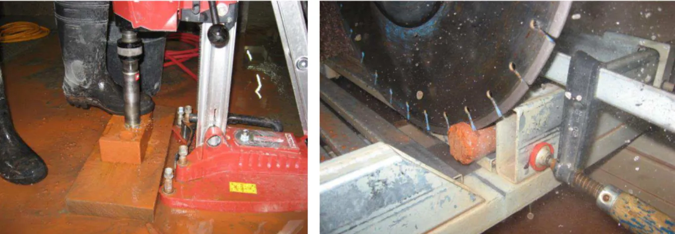
Figure 2.17 presents the used impact system. The impact system consists of a bolt that due to a tensile force, it was romped and produced an impact in the incident bar. Figure 2.18 shows the crack propagation during the dynamic Brazilian splitting test and Figure 2.19 presents the set-up of the dynamic compression test.

Figure 2.18 - Crack propagation during indirect dynamic tensile test, Brazilian test

Figure 2.19 – Dynamic compression test conducted in Split-Hopkinson-Bars

The SHB tests work as follows. At the beginning of the experiment, a high speed impact is applied to the incident bar. Through the impact given at the beginning of the bar, a longitudinal wave ( e) is produced that propagates until it reaches the initial surface of the

specimen. Due to the strain gages, the electrical signals can be obtained and transformed to strain ( ) (Equation (2.17)):

(2.17)

where U0 is the corrected measured voltage;

Cor is the correction factor; U1 is the applied electric voltage;

G is the gain;

Part of the emitted wave is transmitted through the specimen, while the remainder is reflected back. The electrical signals can also be obtained and transformed to strain.

The wave propagation speed (c) produced from the impact system can be obtained from:

√

(2.18)

where E and ρ are properties of the bars, E-Modulus and density, respectively.

Using Equations (2.19) and (2.20), the deformation at the initial (u1) and at the end (u2) of the

specimen (Figure 2.20) can be obtained.

∫ ∫ (2.19)

∫ ∫ (2.20)

Figure 2.20 - Incident strain ( e), reflected strain ( r), transmitted strain ( t) and displacements

(u1 and u2) during a SHB test in a specimen of length Ls

̇ (2.21)

∫

(2.22)

(2.23)

The maximum applied force to the specimen (Fs max) can be obtained by averaging the

maximum applied forces to the bars (Equation (2.24)).

(2.24)

Table 2.9 - Dynamic tensile strength (fst, dyn) obtained for bricks

Specimen h d Fmax ̇ fst, dyn

[mm] [mm] [N] [1/s] [MPa]

T3 43,0 40 10347,78 111,9 3,83 T4 42,1 40 8861,49 110,8 3,35 T5 42,0 40 7679,31 105,9 2,91 T7 42,3 40 10445,10 108,6 3,93 T13 42,1 40 9073,11 116,7 3,43

Average dynamic tensile strength for ceramic brick 3,49

Standard deviation [MPa] 0,41

Coefficient of variation [%] 11,75

A2 39,2 40 8694,42 100,4 3,53 A14 39,1 40 10981,56 99,5 4,47 A21 38,8 40 10507,25 112,4 4,31 A22 39,0 40 6591,69 115,1 2,69 A25 39,1 40 3611,39 99,1 1,47

Average dynamic tensile strength for Afghan clay brick 3,29

Standard deviation [MPa] 1,24

Coefficient of variation [%] 37,69

K2 42,1 40 32642,03 114,4 12,34 K4 42,6 40 30005,10 102,3 11,21 K8 41,7 40 33510,93 104,3 12,79 K9 43,0 40 30016,66 99,5 11,11 K12 42,5 40 31964,13 114,8 11,97

Average dynamic tensile strength for clinker brick 11,88

Standard deviation [MPa] 0,72

Table 2.10 - Dynamic compressive strength (fc, dyn) obtained for bricks

Specimen

d Fmax ̇ fc, dyn

[mm] [N] [1/s] [MPa]

T2 40 30787,61 112 24,5 T11 40 33929,20 82 27 T15 40 38327,43 113 30,5 T17 40 37699,11 60 30 T20 40 34557,52 88 27,5

Average dynamic compressive strength for ceramic brick 27,9

Standard deviation [MPa] 2,4

Coefficient of variation [%] 8,6

A5 40 19603,54 85 15,6 A7 40 24504,42 75 19,5 A23 40 15079,64 100 12

A1 40 21991,15 86 17,5 A16 40 18598,23 93 14,8

Average dynamic compressive strength for Afghan clay brick 15,88

Standard deviation [MPa] 2,8

Coefficient of variation [%] 17,63

Specimen

l Fmax ̇ fc, dyn

[mm] [N] [1/s] [MPa]

K2 21 52479 180 119 K3 21 51597 175 117 K4 21 54243 190 123 K5 21 51597 220 117 K9 21 55125 180 125

Average dynamic compressive strength for clinker brick 120,2

Standard deviation [MPa] 3,6

The coefficient of variation obtained from the Afghan clay brick is very large (Table 2.9). That means that more tests should be conducted.

The results obtained for the tensile strength under dynamic (Table 2.9) and under static (Table 2.5) loads were implemented in Equation (2.16), and the tensile DIF could be obtained. In the same way, the compressive DIF could be obtained, but in this case with the results shown in Table 2.8 and Table 2.10.

The Dynamic Increase Factor obtained for the bricks are shown in Table 2.11.

Table 2.11 - Dynamic Increase Factor (DIF) obtained for the bricks

Bricks

Ceramic Clinker Afghan clay

Tensile DIF 3,03 2,25 1,17

Compressive DIF 1,10 1,38 1,11

Figure 2.21 - Dynamic increase factors for the tensile strength of concrete specimens (black symbols), Schuler et al. (2006), and own tests results for bricks

3

3

M

ATERIAL

M

ODEL FOR

B

RICKS

For this project a modelling approach is needed that is able to simulate masonry walls made of any types of masonry units and any units’ arrangement under dynamic loads. For this vast range of application, including loadings in and perpendicular to the wall, an appropriate modelling strategy is needed. As loadings perpendicular to the plane of the wall cause normal tensile and compressive stresses, it is important to model numerically the interaction between the mortar and the bricks. Therefore, the detailed micro-model strategy, described in Chapter 1, was chosen for the own modelling approach.

As mentioned before, just the material model developed for bricks and its verification and validation are presented. In Linse (2012) the material model developed for mortar is described in detail.

In the following paragraphs the mechanical descriptions implemented in the material model for bricks are presented.

3.1 Definition of stress invariants

In the following a brief definition of the stress invariants used to construct the strength model of bricks will be presented. More information can be find in Chen (1982) and Mai and Singh (1991).

Figure 3.1 - Sketch from a material stress state under triaxial tensile stress (left) and under triaxial compressive stress (right)

In the case of brittle materials, the yield limit depends on the pressure. In this case yielding is described by a yield curve (surface) and not a single point (yield limit). This surface can be represented by Equation (3.1):

(3.1)

where I1 is the first invariant of the stress tensor σij;

J2 and J3 are the second and third stress tensor invariants from the deviatoric stress

tensor sij.

The surface is represented through invariants because the principal stresses (σii) do not depend

on the choice of the coordinate system. I1, J2 and J3 do not change if the coordinate system is

reset, and therefore they are called invariants of the stress tensor (σij). According to Chen

(1982), a yield criterion for isotropic materials based on the tension state, should be an independent function from the coordinate system adopted.

The stress state at any point in a material is defined by the components of the stress tensor (σij).

Per definition, the shear stresses in the principal plane are zero, and then for the direction nj

one has:

(3.2)

where ij is the Kronecker delta, with ij = 1, for i = j and ij = 0 for i ≠ j.

| | (3.3)

|

| (3.4)

The determinant of Equation (3.4) is a cubic equation of principal stresses (σ) with three solutions, I1, I2 and I3:

(3.5)

where

(3.6)

( (3.7)

|

|

(3.8)

If the coordinate system coincides with the principal stress direction one has a hydrostatic stress state and the invariants reduce to:

(3.9)

(3.10)

(3.11)

The stress tensor (σij) can be expressed as the sum of a purely hydrostatic stress (σm) and a

deviation from the hydrostatic state (sij).

(3.12)

₍ (3.13)

where σm is the mean stress or the hydrostatic stress;

sij are the deviatoric stresses, which represents a state of pure shear.

(3.14)

| | (3.15)

(3.16)

where

(3.17)

_[( ( ] (3.18)

|

|

(3.19)

If the coordinate axes coincide with the principal direction ni, one obtains

(3.20)

[ ]

(3.21)

(3.22)

The determination of the principal stresses, Equation (3.5) and Equation (3.16), is not so easy. However, a similarity between Equation (3.16) and a trigonometric identity is observed:

(3.23)

If s = ρ.cos is substituted in Equation (3.16) one has:

(3.24)

Comparing Equation (3.23) with (3.24) one has:

√ √

√ (3.26)

If 0 represents the first root of Equation (3.26), for the angle 3 in the interval between 0 and

π, 0 must vary within the interval

(3.27)

Observing the natural cycle of cos (3 0 ± 2nπ), the only three possible values of cos that

give the principal stresses are:

(3.28)

(3.29)

(3.30)

With the limitation of 0 imposed by Equation (3.27), one has:

[ ] [ ] [ ] √ √ [ _] (3.31)

with σ1≥ σ2 ≥σ3. Equation (3.31) has three stress invariants:

(3.32)

√ (3.33)

(3.34)

( √ (3.35)

(3.36)

In order to represent the hydrostatic (Equation (3.13)) and deviatoric (Equation (3.14)) stress states and the angle of similarity ( ) (Equation ((3.26)), the projection on the deviatoric plane

of the coordinate’s axes σ1, σ2 and σ3, and the stress decomposition in the principal stress

space are presented in Figure 3.2. The hydrostatic (ξ) and the deviatoric (ρ) axes represent the Haigh-Westergaard stress space.

Figure 3.2 - Projection on the deviatoric plane of the coordinate’s axis σ1, σ2and σ3 (left) and

stress decomposition in the principal stress space (right)

An octahedral stress plane makes equal angles with each of the principal axes of stress and it can also be represented like the deviatoric plane. However, if one compares the Haigh-Westergaard coordinates with the octahedral coordinates, the following relations will be find:

√ (3.37)

√ (3.38)

The octahedral normal stress and shear stress can be obtained with Equations (3.39) and (3.40).

√

(3.40)

The direction of the octahedral shear stress is defined by the angle of similarity

√

(3.41)

In this way, the function represented by Equation (3.42) can also represent a yield surface of brittle materials.

(3.42)

3.2 Strength model

The general form of the yield surface for brittle materials in three dimensional stress space can be better described by the form of the cross-section in the deviatoric plane, which is perpendicular do the hydrostatic axis, and its meridians are in the meridian plane.

The meridians of the yield surface are the curves of intersection between the failure surface and a plane (including the meridian plane) including the hydrostatic axis with constant .

Figure 3.3 - Representation of the material test position on the stress surface, Linse et al. (2012)

For the purpose of the strength model development, approaches that could be found in the literature were analyzed. The ceramic material model published by Johnson and Holmquist (1993) and the model by Hao and Tarasov (2008) were investigated by Linse. Both models are based on assumptions that are not quite valid for the bricks purpose.

Finally, the Ottosen-Speck model was chosen, which comprises the Ottosen model with an extension by Speck (2007). For this model, a wide range of applications for normal and ultra-high performance concretes is proven. The fracture surface is defined by

_| | √ | | | | (3.43) with (3.44)

for > ° nd

( ) (3.45)

for < °.

In order to fit the brick strength model, test data for at least four different stress states are necessary: uniaxial tensile, uniaxial compressive, biaxial compressive and triaxial compressive tests.

The necessary material parameters to calibrate the Ottosen-Speck model are: the uniaxial tensile strength ( ), the uniaxial compressive strength ( ), the biaxial compressive strength ( ) and three dimensional compressive test on the compressive meridian, defined by and

. Having these test data, the calibration can be done with the following equations:

√ √ | | _| | √ √ (3.46)

_{| | | | | | | |} (3.47)

[ n

√ )]

(3.50)

[ ( ) ] [ ( )] (3.51)

The uniaxial stress states were determined with own material tests, presented in Chapter 2. For the other stress states, Linse (2012) made assumptions based on comparisons with concrete and sand. The results are presented in Table 3.1.

Table 3.1 - Material parameters for masonry units, Linse (2012)

Ceramic Clinker

German

clay

Afghan

clay

Concrete

fc [MPa] -34,8 [1] -94,5[1] -2,4 [1] -10,1 [1] -38,7

ft [MPa] 1,1 5,5 0,3 1,4 2,2

fcc [MPa] [2] -1,16 x fc -1,1 x fc -1,25 x fc -1,25 x fc -1,16 x fc [3]

0 [MPa] [4] -2,887 x fc -103,5 [5] -3 x fc -3 x fc -2,887 x fc [3]

0 [MPa] [4] 2,31 x fc 89,6 [5] 3 x fc 3 x fc 2,31 x fc [3]

[1] 80% of the obtained compressive strength, according to DIN V 105-100 (2005) [2] analogy based on different types of concretes, Linse (2012)

[3] test data for concrete

[4] extrapolation of concrete test data [5] test data for high performance concrete

3.3 Tension cut-off with Rankine criterion

Bricks are brittle materials and they usually fail under laterial tension. Therefore, a tensile failure surface, also known as tension cut-off criterion, was used.

The tensile strength of the bricks is described by the Rankine criterion (principal stress criterion) (Equation (3.52)).

√ (3.52)

where I1 is the first invariant of the hydrostatic stress tensor;

J2 is the second invariant of the deviatoric stress tensor;

is the angle of similarity and is the tensile strength.

3.4 Elastic and plastic material status, residual strength and damaged

material status

The material stress-strain behavior can generally be characterized by three domains: elastic, plastic and damaged (Figure 3.4). This characterization is not so clear if the transition between the domains is not clearly identifiable.

Under tensile loadings, bricks do not show a plastic domain. They seem to behave elastically until brittle fracture. Under compression, some plastification can be observed.

Figure 3.4 - Schematic representation of the material status, the fracture strains, the residual strength and the strain when residual strength is achieved, Gebbeken et al. (2011)

This model is based on assumptions and comparisons with Bierwirth (1995)’s test data for mortar. In the near future triaxial test data for bricks will be used and the assumptions can be controlled.

Figure 3.5 shows the effective fracture strain ( eff,B) as a function of triaxiality . In this

Figure 3.5 - Effective fracture strain as a function of triaxiality ( ), Gebbeken et al. (2011)

He conducted the tests using a pressure cell and applying different confining pressures. These tests show that the fracture strains increase with a decrease in triaxiality. In order to describe the fracture strains for every stress state, the following values are needed:

Fracture strain, uniaxial tensile test; Fracture strain, uniaxial compression test; Fracture strain, triaxial compression test;

Triaxiality by fracture, uniaxial tensile test (0.333);

Triaxiality by fracture, uniaxial compression test (-0.333); Triaxiality by fracture, triaxial compression test (-0.51).

The interpolation of the measured data points of the effective fracture strains is described by linear functions (Equation (3.53)). These four functions are plotted in Figure 3.5.

In the two small diagrams in Figure 3.5, which show Bierwirth’s material tests, the influence of the stress state on the residual strength can be observed. Table 3.2 shows the results of the

residual strength for Bierwirth’s material tests. These values correspond to the colored crosses and circles in Figure 3.5.

Table 3.2 - Residual strength for different stress states, based on Bierwirth’s material tests

Uniaxial

compression

Confining pressure / Principal stress

(σr/ σv)

0,05 0,15 0,3

Triaxiality (η) -0,333 -0,386 -0,51 -0,762

Residual strength (fR) 0,35 0,67 1 1

This data leads to the following system for the residual strength:

{ >

(3.54)

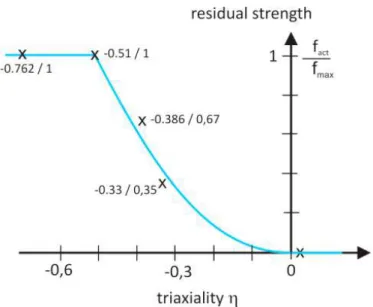
Equation (3.54) is illustrated in Figure 3.6. According to Linse (2012), the definition of the residual strength after fracture is one of the complicated tasks that were encountered during

Figure 3.6 - Residual strength as a function of the triaxiality of the stress state, Gebbeken et al. (2011)

Concluding remark: If the material behavior after fracture should be described, the fracture strains, the residual strength and the strain at which the residual strength is achieved are important material properties that are needed.

Figure 3.4 shows schematically the material post fracture behavior for several stress states. These material properties must be determined with experiments for one, two and three dimensional stress states. Table 3.3 shows estimations for masonry bricks, Linse (2012).

Table 3.3 - Fracture strains for masonry bricks

Ceramic Clinker German clay Afghan clay Concrete

eff,B,1Z [6] 9,0 x 10 -4

1,58 x 10-4 5 x 10-4 0,38 x 10-4 0,178 x 10-4

eff,B,1D [4] 9,5 x 10 -3

4,0 x 10-3 3 x 10-3 1,5 x 10-3 2,3 x 10-3

eff,B,3D [3] 19,0 x 10 -3

8,0 x 10-3 6 x 10-3 3,0 x 10-3 4,6 x 10-3

Up to now, the values eff,B and eff,R are estimated for the bricks for 3-dimensional stress

The damage model is needed to describe the decay of the material strength and the material stiffness after fracture. It is assumed that the material damage (D) begins as is exceeded. The developed damage model is based on the effective strain of the material.

There are two input parameters for the model: and . The latter is the effective strain when the residual strength is achieved. These two effective strains are quite different for different stress states and must be distinguished for compressive and tensile states (Figure 3.7).

Figure 3.7 - Adaption of the fracture surface due to material damage for several stress states, Gebbeken et al. (2011)

3.5 Adaption of the material stiffness

After fracture, a decay of the material stiffness is observed. Compression tests stress-strain diagrams of Oliveira (2003) show that the stiffness decreases significantly.