The efect of the financial crisis on Croatia ’s primary budget deficit and public debt

(1)

PRIMARY BUDGET DEFICIT AND PUBLIC DEBT

Petar SOPEK, student* Article**

Faculty of Science, Zagreb JEL H63

UDC 336.27(497.5)

Summary

The basic aim of this article is to consider the effect of the current financial crisis on the movements and sustainability of the public debt in the period up to 2013. It is shown that changes in the public debt come from the effect of the primary deficit created, stock-flow adjustment, the real growth of the GDP and real interest rates. On the basis of re-sults of the European Communities (2009) a statistical estimate is given of the trends in the primary deficit for EU-12, after which the model is adjusted to Croatian figures. The projection of stock-flow adjustment is undertaken from a projection of the primary defi-cit, due to the relatively strong negative correlation between those two variables in the past, whilst the projection of the real growth rate of the GDP and real interest rates is sig-nificantly simplified. The main hypothesis tested is that the ratio of the public debt in the GDP up to 2013 does not exceed the margin of sustainability prescribed in the Maastricht criterion of 60%, which is finally confirmed by this analysis.

Key words: Public debt, fiscal sustainability, primary deficit, stock-flow adjustment, the Croatian economy.

Introduction 1

In the period from 2002 to 2008 and especially after 2004, the indicators of the defi-cit and public debt in Croatia improved (Ministry of Finance, 2009a, 2009b). But this en-tire period, excluding 2008, was characterised by high real growth of the GDP (on aver-age 4.8%) and relatively low inflation (on averaver-age 2.5% in comparison with the EU av-* I would like to thank two anyonymous referees for their helpful and constructive comments. I would also like to thank the Institute of Public Finance, which has provided a supportive environment for this research.

** Received: June 18, 2009

(2)

Financial Theory and Practice 33 (3) 273-298 (2009)

erage of 2.1% 1_{). At the beginning of 2008 inflation began to rise and that year it recorded} a rate of as much as 6.1%, which is enormous growth in comparison with the inflation rate of 2.9% in 2007. On the other hand, the annual growth of the real GDP was only 2.4%, which was a large fall in comparison with 5.5% in 2007 (CBS, 2009b). In 2008 it became clear to everyone that the crisis was spreading from the mortgage market in the USA and that it would affect the rest of the world much worse than was thought.

Most European countries already began to feel the overflow of the crisis onto their own backs at the beginning of 2008, whilst in Croatia at that time the crisis was mainly only being felt on the stock markets, which recorded significant losses, following the ex-ample of the world markets. The two largest economies in Europe, Italy and Germany, al-ready recorded a fall in economic activity and fell into recession in the second and third quarters of 2008 (Euromonitor International, 2009), but Croatia not until the last two quar-ters of 2008 (---, 2009a) 2_.

It is generally known that in times of crisis state revenues decrease, whilst expend-iture from the state coffers continues to increase. This happens for several reasons: the growth of unemployment, the increasing demands for fiscal incentives, the growth of interest rates etc. All this leads to growth of the deficit, and thereby to growth of the public debt. The main aim of this article is to consider the effect of the current financial crisis on the movements and sustainability of the public debt in the period to 2013. The Maastricht criterion set the margin of sustainability of the public debt in the GDP at 60%, but it should be emphasized that that margin is not necessarily any guarantee of sustainability. That is to say, in as many as 55% cases of government bankruptcy the level of the public debt was below 60%, and in as many as 35% cases even below 40% (IMF, 2003).

The main hypothesis tested in this article is that the ratio of the public debt in the GDP will remain below the level of 60% until 2013, whereby, according to the Maastricht cri-terion we can take it as satisfactory. This gives rise to logical questions such as: which variables have a significant influence on the movements of the public debt, how will the current financial crisis affect the movements of those variables, is there any connection between them and how great is the insecurity of future projections?

It is seen that the movements of the public debt are most significantly affected by the primary budget deficit and the stock-flow adjustment, and less, but not without signifi-cance, by the real GDP growth rate and real interest rates on the public debt. It is shown statistically that Croatia’s primary deficit in the period 2006-2009, with some additional alterations, follows a similar path to the primary deficit of EU-12 member states in the pre-crisis period. Adjustment of the EU-12 model leads to a projection of the Croatian primary deficit. A negative correlation is also shown between the variables of primary deficit and stock-flow adjustment in the past, which, under the assumption that this trend will remain the same in future, significantly facilitates the projection of the public debt

1_{The inflation rate measured by the consumer price index (Sources: Central Bureau for Statistics (CBS), 2009a,} for Croatia, and Eurostat, 2009a for the EU).

(3)

and modelling of the sources of uncertainty of the estimate. The final results gained show that even at the upper limit of the 99 percent confidence interval, the ratio of the public debt in the GDP remains below the level of 60%, whereby we cannot reject the hypoth-esis of its sustainability. However, in view of the short time series, and the method which relies mainly on statistics rather than macroeconomic analysis, the results should be in-terpreted with additional caution.

The article is arranged as follows: after the introduction, the second part of the arti-cle considers the effect of the crisis on trends in the primary deficit based on the results of the European Communities (2009). In the third part, an attempt is made to adjust that effect statistically to Croatian figures, from which the projection is drawn. The fourth part links the primary deficit with the stock-flow adjustment and offers assumptions for the other variables, and then creates a projection, together with the confidence interval. This is followed by a conclusion.

Primary deficit in times of crisis 2

A financial (banking) crisis can be defined in several different ways. The definition which this article relies on describes a crisis as various episodes in which the financial and corporate sectors of individual states face major difficulties with the timely payment and collectability of their agreed debts, a significant increase in the number of unused loans and the exhaustion of most of the capital of the banking system. Financial crises mainly occur in developing markets, but they also affect other markets and even more developed countries such as EU or OECD member states can feel a crisis (Laeven and Valencia, 2009).

The European Communities results (2009) from which the conclusions in this article will be drawn, are founded on earlier articles, of which it is important to mention Laeven and Valencia (2008), Demirgüç-Kunt and Detragiache (2005) and Reinhart and Rogoff (2008). There are other interesting articles in this field, but the results arising from these are the most interesting as they supplement a consideration of the effect of the crisis with exceptionally quality and comprehensive empirical analysis, which will also be relevant for this article.

The empirical analysis (European Communities, 2009) covers a total of 49 crisis ep-isodes, between 1970 and 2007, of which 22 were in EU-27 and OECD member coun-tries, where it is estimated that the average duration of the crisis was four and a half years. It is important to emphasize that EU-15 signifies crisis episodes in Finland, Spain and Sweden, from 1970 to 2007, whilst EU-27 signifies crisis episodes in Bulgaria, Czech Republic, Latvia, Lithuania, Hungary, Poland, Romania, Slovakia, Slovenia, Spain and Sweden, where for the new members (all except Finland, Spain and Sweden) the period from 1991 to 2007 is analysed.

(4)

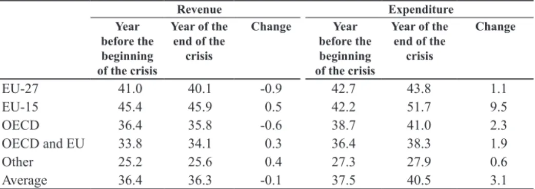
Table 1 Total revenues and expenditure before and after the crisis (% of GDP)

Revenue Expenditure

Year before the beginning of the crisis

Year of the end of the

crisis

Change Year

before the beginning of the crisis

Year of the end of the

crisis

Change

EU-27 41.0 40.1 -0.9 42.7 43.8 1.1

EU-15 45.4 45.9 0.5 42.2 51.7 9.5

OECD 36.4 35.8 -0.6 38.7 41.0 2.3

OECD and EU 33.8 34.1 0.3 36.4 38.3 1.9

Other 25.2 25.6 0.4 27.3 27.9 0.6

Average 36.4 36.3 -0.1 37.5 40.5 3.1

Source: European Communities (2009)

The Table indicates the fact that revenue on average was slightly reduced, whilst ex-penditure in all the groups considered increased, and the average increase was about 3% of the GDP. Since only the year before the beginning of the crisis and the year of the end of the crisis are shown, the increase in expenditure and the reduction in revenue are rela-tively small, but it is realistic to assume that in the first years of the crisis the increase in expenditure and reduction in revenue were much greater, after which they stabilized to the values shown in the Table.

The difference in total revenues and expenditure according to the ESA methodology shows the budget balance (European Communities, 2002). If there is an excess of reve-nue over expenditure we say that a budget surplus has been attained, whilst for a shortfall of revenue we use the term budget deficit. An important indicator is what we call the pri-mary budget balance, which shows the budget balance not including the calculation of expenditure on interest, that is the difference between total revenues and total expenditure reduced by expenditure on interest. In this article instead of the phrase (primary) budget balance, we will use the expression (primary) budget deficit, although in the case of a pos-itive outcome it actually refers to a budget surplus. The budget and primary budget bal-ance in times of crisis are shown in Table 2.

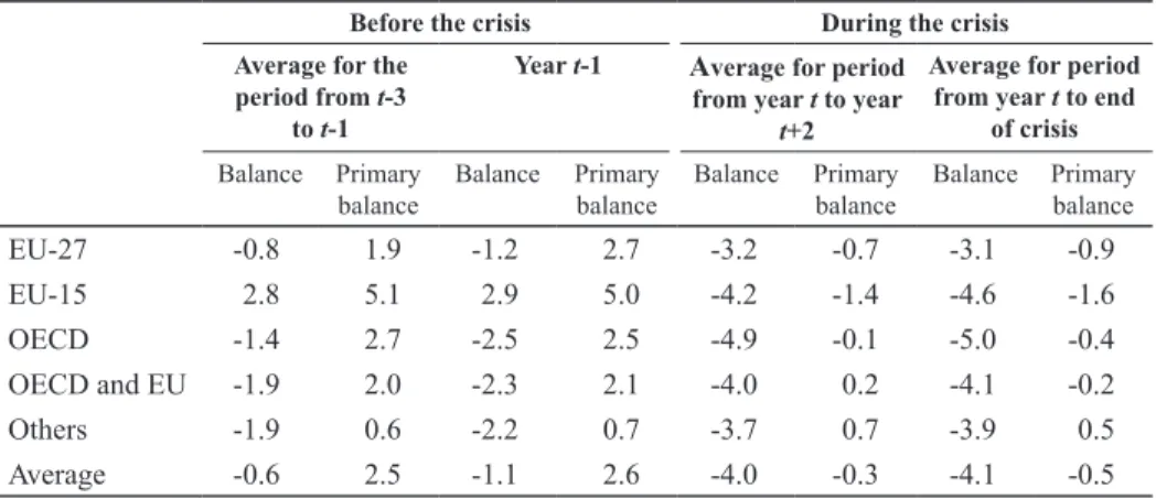
In all the groups in question in the year when the crisis ended there was a budget def-icit, regardless whether there was a deficit or surplus in the years before the beginning of the crisis. It is interesting that in the EU-15 the greatest difference was found in the budg-et balance from the pre-crisis year to the year of the end of the crisis, amounting to as much as 7.5 percentage points. The pace of change in the primary budget balance is shown in Graph 1, with the addition of the pace of changes in the primary budget balance for EU-123_.

(5)

Table 2 Budget balance and primary budget balance in times of crisis (% of GDP)

Before the crisis During the crisis

Average for the period from t-3

to t-1

Year t-1 Average for period from year t to year

t+2

Average for period from year t to end

of crisis

Balance Primary balance

Balance Primary balance EU-27 -0.8 1.9 -1.2 2.7 -3.2 -0.7 -3.1 -0.9

EU-15 2.8 5.1 2.9 5.0 -4.2 -1.4 -4.6 -1.6 OECD -1.4 2.7 -2.5 2.5 -4.9 -0.1 -5.0 -0.4 OECD and EU -1.9 2.0 -2.3 2.1 -4.0 0.2 -4.1 -0.2

Others -1.9 0.6 -2.2 0.7 -3.7 0.7 -3.9 0.5 Average -0.6 2.5 -1.1 2.6 -4.0 -0.3 -4.1 -0.5

Source: European Communities (2009)

The pace of changes in budget and primary budget balances indicates a drastic fall in the initial years of the crisis (the first 2-3 years), after which it begins to stabilize with minor oscillations. As has already been mentioned above, the estimated duration of the crisis in EU countries and the OECD is four and half years, and from Graph 1 it is clear that even after five years from the beginning of the crisis the budget balance does not suc-ceed in reaching the level of the pre-crisis years.

Graph 1 Changes in primary budget balance in times of crisis (%GDP)

6

5

4

3

2

1

0

-1

-2

-3

-4

t - 4 t - 3 t - 2 t - 1 t t + 1 t + 2 t + 3 t + 4 t + 5

EU-15 EU-27 EU12

(6)

Financial Theory and Practice 33 (3) 273-298 (2009) Projection of the

3 Croatian primary deficit

We have seen that the occurrence and intensifying of a crisis has an important effect on the movements of the primary deficit. Here in the sample under consideration, the pe-riod of the first two years is most critical, after which there is a gradual stabilization, but full recovery to the level of the pre-crisis years can take as much as one decade. But can the previous experiences, considered above, be used to assess the effect of the current fi-nancial crisis? Our desire, using the data available for the period up to 2008, and an esti-mate for 2009, is to offer a framework of the probable effect of the crisis on the movements of the primary deficit, and then the public debt of Croatia. According to the Budget Act (Official Gazette 87/08), the public debt or the debt of the public sector from 1st_January 2009 comprises the debt of the general government, which no longer includes the so-called potential debt in the form of financial and factual guarantees issued, and the debt of HBOR.4 The public debt changes over a certain time period due to the deficit realized and changes to some other variables in that time period, which we will say more about in Section 4.

3.1 Modelling trends in the primary deficit of EU-12

Graph 1 shows the trends in the primary budget balance which may be very well ap-proximated by a polynomial function of the third or higher degree. We will use a polyno-mial of the fifth degree in the text below, since it appears that it almost perfectly describes the data from the EU member countries in the period in question, and moreover it proves to be much better when adjusting to the Croatian figures. Polynomial regression is actu-ally a special case of multiple linear regression5_{, which in the case of our time series of} figures may be written as the following expression:

X =β βt β t βt βt βt ε

0 1 2

2 3

3 4

4 5

5

+ + + + + + (1)

where represents the vector of the primary budget balance (as a percentage of the GDP), is the vector marking the moment of time (-4,-3,…,5), βk are unknown coefficients (for k

= 0,..., 5), and ε represents the vector of random errors. With the sample given, by the method of the smallest squares the unknown parameters βk are estimated.

Since the EU-12 countries are most similar to Croatia in terms of their transitional past and living standard (Eurostat, 2009b), we will consider the trend of movements of primary deficit for the EU-12 and compare it with figures for Croatia. It is shown that this model, with small alterations, is really the best approximation of the primary deficit real-ized in Croatia for the period from 2006-2009.

By an estimation of the unknown polynomial regression for the EU-12 we gain the following expression:

X =0 8445 1 2824t 0 1364t2 0 0923t3 0 0104t4 0 0

, – , – , + , + , – , 0035

t –e (3.31**) (-6.38***) (-1.64) (2.64*) (2.17*) (-2.08)

(2)

4_{In line with the Act on the Croatian Bank for Reconstruction and Development (HBOR) (OG 138/06) the state} guarantees all its debts, so the HBOR debt is frequently added to the total amount of guarantees.

5_{With the replacement t}

(7)

where Xand t are vectors, as above, but is a residual vector, or deviations from the ex-pected value. The values in brackets below the parameters signify the values of t-statis-tics, with the sign * for levels of significance up to 10%, ** for levels of significance up to 5% and *** for levels of significance up to 1%. The graphical presentation of the values attained and the estimated function of the primary deficit of the EU-12 in the pre-crisis and pre-crisis years is shown in Graph 2. As before, the sign t is used for the first year of the crisis.

Graph 2 Realized and estimated primary deficit of EU-12 (% GDP)

4

3

2

1

0

-1

-2

t - 4 t - 3 t - 2 t - 1 t t + 1 t + 2 t + 3 t + 4 t + 5

Source: European Communities (2009); the author

The estimated primary deficit for the EU-12 already shows signs of a negative trend from the second year before the crisis, but there is only dangerous growth between the first year before the crisis and the year the crisis began. The highest primary deficit real-ized is expected between the second and third year of the crisis, after which it stabilizes. The function from the picture which best describes the movements of the primary deficit of EU-12 countries is a special case of expression (2):

f t( )=0 8445 1 2824, – , t–0 1364, t2+0 0923, t3+0 0104, t4 – 0 0 0035

, t (2’)

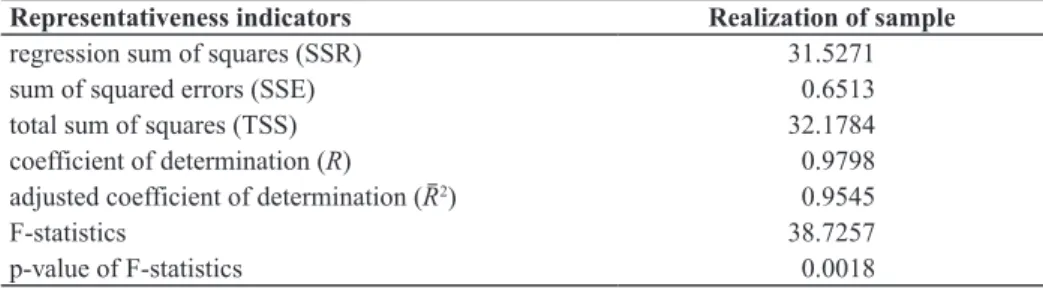
At first sight it seems that the model describes very well the real values in the period in question, since all results are quite close to the estimated functions. The representative-ness indicators of the model shown in Table 3 will serve as evidence of this.

(8)

1.8%.6_{All this further supports the quality of the model. It remains to verify whether the} residuals satisfy the characteristic of normality, which is one of the preconditions of a re-gression model, which is confirmed by the Kolmogorov-Smirnov test (KS), and at the level of significance up to 8.4% we cannot reject the hypothesis that the data (residuals) come from a standard normal distribution. In other words, the assumptions of the regres-sive model are also satisfactory to that level of significance.

Table 3 Representativeness indicators of the model to describe the movements of the primary deficit of EU-12

Representativeness indicators Realization of sample

regression sum of squares (SSR) 31.5271

sum of squared errors (SSE) 0.6513

total sum of squares (TSS) 32.1784

coefficient of determination (R) 0.9798 adjusted coefficient of determination (R2₎ _0.9545

F-statistics 38.7257

p-value of F-statistics 0.0018

Source: author’s calculation

3.2 Adjustment of the model to Croatian figures

The next task is to adjust the estimated function for the EU-12 so that it best suits the primary deficit realized by Croatia. Since no fall in economic activity in Croatia was re-corded until the third quarter of 2008, for the beginning of the crisis we took the middle of 2008.7_{Our starting point is the assumption that the model describing the movements} of the primary deficit of Croatia in the pre-crisis and crisis years is a vertical shift down-wards (linear transformation with a unit linear member) of the function (2’), given in the following expression:

_{f t}_{( )}₌ _{f t}₍ _–_{2008 5}_, ₎_–_w ₍₃₎

where t signifies the year and w the vertical shift. The assumption that the primary deficit will follow a similar curve seems economically reasonable in view of the fall in budget revenues and growth of expenditure in the first year of the crisis. Apart from that, in the movements of the primary deficit a fall is also implicitly included in the calculation, that is, the realization of lower levels (in relation to the average) of growth of the real GDP in that period. However, this method of projection of the primary deficit is mainly founded on statistical estimates, since we consider most macroeconomic variables as given, that is as exogenous variables. It is however necessary to point out that good quality fiscal

poli-6_{F-statistics test the null hypothesis H}

0: β1 = β2 = ... = β5 = 0, that is the acceptance of the null hypothesis would mean that the model does not depend significantly on the assumed variables but only on a free member.

(9)

cies may have a major effect on future trends in the primary deficit, which we will say more about later.

In order to find the optimal vertical shift w*, we need to find the minimum of the fol-lowing expression (function g), which gives the squared deviation of the realized figures from the estimate:

min min – , – ,

w w

p p

g w( )=

(

b2006 f(- )+w

)

+ b f(- )

2 2007

2 5 1 5 ++

+ - + + +

w

bp f w bp f w

(

)

( )

(

)

(

( )

)

2

2008

2 2009

0 5 0 5

– , – , 22

(4)

For the purpose of this analysis an “adjusted” primary deficit was calculated (bt p

) for 2006 and 2007, which excludes Croatian Motorways (HAC) from the general govern-ment.8_{For 2009 a projection was made based on the information available, and it includes} a fall in the real GDP of 5% and an inflation rate of 3% (---, 2009b) and the third rebal-ance of the state budget (Ministry of Finrebal-ance, 2009c), with an assessment of the ratio of revenues and expenditure of the state budget in the budgets of general government (on average about 85%). In this way a total deficit was reached of 11 billion kuna (3.3% of the GDP), that is, a primary deficit of about 5 billion kunas (1.6% of the GDP).

The function (g) which we minimize in the expression (4) is actually a polynomial function of the second degree with a unit coefficient in front of the square member (the parabola turned upwards), which means that there is a single minimum. The graphical pres-entation of this function at the interval containing the minimum is shown in Graph 3.

Graph 3 Function of adaption of RoC figures to EU-12 figures

1

0,5883

1 1,4171

g_min (w)

2

Source: The author

(10)

The calculated minimum of the function g is attained for and amounts to w* = 1,4171 and amounts to g(w*) = 0,5883. This in fact means that, with the assumption mentioned earlier, the function which describes the expected trends in the primary deficit in Croatia is given by the following expression:

 

f t f t

f t t

( ) ( )

( )

= =

-– –

– –

, ,

2008 5 1 4171

0 5726 1 2824( 20008 5, )–0 1364, (t–2008 5, )2+0 0923, (t–2008 5, )3 +0 0104, (t+2008 5, )4–0 003, (t–2008 5, )5

(5)

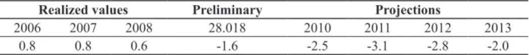
For the EU-27 the calculated minimum is 0.75 which confirms that the assumed model of the EU-12 is indeed better, since the squared deviations of adjustment to Croatian fig-ures are smaller. The graphical presentation of the primary deficits of Croatia from 2006-2009 and the projection for the period 2010-13 on the basis of the adjusted function of trends in the primary deficit is shown in Graph 4.

Graph 4 The primary deficit realized and projected (% of the GDP), 2006-13

3

2

1

0

-1

-2

-3

-4

2006 2007 2008 2009 2010 2011 2012 2013

Source: the author

(11)

Table 4 Projection of the primary deficit of Croatia (% of the GDP)

Realized values Preliminary Projections

2006 2007 2008 28.018 2010 2011 2012 2013

0.8 0.8 0.6 -1.6 -2.5 -3.1 -2.8 -2.0

Source: the author’s calculation

3.3 Stochastic model of trends in primary deficit

Now, when we know the expected trends in future primary deficits, we would like to create a stochastic model of those trends, with the assumption that the expected values of the future primary deficit are well described by function (5) and that the residuals (devia-tion of the realized from the expected values of the primary deficit for previous years) fol-low the standard normal distribution. With these limitations, there is sense in assuming that the future deviations of realized values from function (5) will also be normally dis-tributed, but since these are projections, the excepted value of the primary deficit in year

t + k is formed by including the trend (function (5) with a vertical shift) in the realized values of primary deficit in year t + k − 1. One simulated example of forming the expect-ed future deficit with simulatexpect-ed realizexpect-ed values, is shown in Graph 5.

Graph 5 Simulation of trends in primary deficit and formation of expectations (% GDP)

3

2

1

0

-1

-2

-3

-4

2009 2010 2011 2012 2013

(12)

the expectations of future primary deficits are formed on the basis of the last known val-ues and trends of movement, and deviation from the expected valval-ues (not the initial as-sumed function) have standard, normal distribution.

Let bt p

signify the last known realized value of the primary deficit (in our case this is the preliminary value for 2009). Then this is actually realization of the random variable

Xj defined by the following expression:

X_t = f t( )+ε_t ₍₆₎

where ε_t~ N(0,1) is the standard normal error, and f t( ) the function defined by expres-sion (5).

According to the assumptions given above, the value of the primary deficit in year

t + 1 is the random variable Xt+1 given in the following expression:

Xt+1= Xt+ f t( +1)– f t( )+εt+1 (7)

where f t( + 1)– f t( ) signifies the change in primary deficit due to the included trend. Analogue to this, we can express the value of the primary deficit in year t + 2 as the ran-dom Xt + 2 variable as follows:

Xt+2= Xt+1+ f t( +2)– f t( +1)+εt+2 (7’) And combined with formulas (6) and (7) gives:

Xt+2= f t( +2)+ε εt + t+1+εt+2 (7’’) Therefore, in year t + k the primary deficit represents the random variable Xt + k shown

by the following expression:

X_{t k} f t k

i t t k i +

= +

( )

∑

=  + + ε (8)

That is, the primary deficit in year t + k is equal to the total of the expected value of the primary deficit in year t + k, the measured function f and deviation consisting of the sum of k + 1 independent standard normal random variables. Since X_t₊_kis also a random var-iable, we are interested in its distribution, and it clearly depends on the sum of errors.

For this the known results of statistical theory will serve. Let Ni ~N μ( ,i σi)

2 ,

i = 1,…, m be the series of independent random variables from normal distribution. Then the sum of those random variables is also a normal random variable with an expectation which is the sum of the expectations of all Ni and the variation which is the sum of the

variations. That is, the following expression applies:

N₁ N₂ N_m N μ₁ μ₂ μ_m ₁2 _m

2

2 2

(13)

From expression (9) follows in particular:

i t t k

i N k

= +

∑

ε ~ ( ,0 +1) (9’)

Which in combination with the equation (8) gives:

Xt k+ ~N f t

(

( +k k), + 1

)

(10)

In other words, Xt + k is a normal random variable with expectation of f t( +k) and

standard deviation k+ 1 . We note that in this analysis we assume the Markov property of the random variable Xt k+ ,∀ ∈k 0, that is behaviour in the future depends on the last known realized value and not on all earlier moments.

From formula (10) it is clear that the distributions of primary deficits for all future years have increasingly heavy tails which means that the reliability of the estimate in all future time periods is subject to increasing deviation from the expected values. As a re-sult we want to construct (1-α_{)% confidence intervals (for various values of}α∈ 0 1, ) for the primary deficit, which actually signifies the interval which, with the probability (1-α_{)% will contain the value of the primary deficit in each year. This may be described} as follows:

P –z Xt k– t k z –

t k

α α

μ σ

2≤ ≤ 2 =1

⎛ ⎝ ⎜⎜ ⎜⎜ ⎞ ⎠ ⎟⎟⎟ ⎟⎟ + + + α (11)

where μt k+ = f t( +k)are the expectations of random variables Xt + k, σt k+ = k+ 1 the

standard deviation of the random variable ( ) ⋅ ( ) Xt + +k, a ⋅z

⎡

⎣⎢ α2 1 α2 the appropriate quantile of standard ⎤⎦⎥

normal distribution.

By slight transformations of the expression within the brackets (11) we obtain:

P

(

_{f t}₍ ₊_k₎ _k₊ _⋅ _≤ _≤₍ ₎ _⋅

)

+

– 1 _α _α α

P  _z _X _{f t} _k _k

t k

+ + + +

( ) ⋅ ≤ ≤ ( ) ⋅

(

1 + 1

)

1

2 2

α α α

P

(

₍ ₎ _⋅ _≤ _≤₍ ₎ ₊ _⋅_z

)

₌

+ 1 1–

2 2

α α α

x x (11’)

From here it now follows that (1-α)% is the confidence interval for X_t₊_kequal to:

x x

 

f t( +k) k+ ⋅ ( ) ⋅

⎡

⎣⎢_⎣⎢⎡( –) +11⋅αz , f t( +k)+ k+1⋅α ⎤⎦⎥⎤_⎦⎥

2 2

α α

₍ ₎ _⋅ ₍ ₎ ₊ _⋅_z

⎡

⎣⎢ α2 1 α2⎤⎦⎥ (12)

Graph 6 shows the expected values of the primary deficit in 90, 95 and 99% confi-dence intervals for the period 2009 to 2013.

(14)

Graph 6 Confidence intervals for trends in primary deficit (% of GDP) 2009-2013

4

2

0

-2

-4

-6

-8

2009 2010 2011 2012 2013

99% confidence interval 95% confidence interval 90% confidence interval primary deficit projection primary deficit 2009 (preliminary)

Source: author

Projection of the public debt 4

It is not possible to undertake a statistical analysis like this without any reference to macroeconomic variables, such as we used for the trends in movements of the primary deficit in the case of the public debt. In other words, it is not possible to take the trend of movements for country members of the EU-12 and simply adjust it so that it suits the Croatian figures as best as possible. First, the public debt depends on a significantly larg-er numblarg-er of macroeconomic variables than the primary deficit. Second, the public debt at the end of each year is closely related to the amount of the public debt at the end of the previous year, whilst the primary deficit changes for each year, depending on the realiza-tion of total revenues and expenditure in the current year. So the vertical movements of the trend of movements of the public debt, even with the assumption that the amount of the debt only changes by the amount of deficit realized, due to the amount of expenditure on interest (which depends on the level of the public debt) and the difference in the reali-zation of the primary deficit (which according to the projections is higher than in the EU), would lead to completely wrong conclusions. For this reason the analysis of the trend of movements of the ratio of the public debt in the GDP should be formed independently of trends in other countries and by including all relevant variables.

In order for us to describe the movements of the public debt, it is not sufficient only to consider the amount of primary deficit realized and the amount of expenditure on in-terest (Babić et al., 20039_{). For this reason we will use slightly extended, known formulas}

(15)

for movements in the public debt (Mihaljek, 2003.) so we therefore assume that the ab-solute value of the nominal amount of the debt at the end of year t is equal to the absolute value of the nominal value of the debt at the end of the year t – 1 reduced by the budget balance achieved (primary budget balance less expenditure on interest) increased by stock-flow adjustment (Eurostat, 2009c.). In other words, according to this formula:

Dt Dt Bt K S

p

t t

= −1–( – )+ (13)

where Dt signifies the amount of the debt at the end of year t, Bt p

the primary budget bal-ance realized, Kt the amount of expenditure on interest, and St stock-flow adjustment in

year t. Stock-flow adjustment is a generally measurable variable, consisting of the net course of financial assets and various other adjustments (transactions in financial deriva-tives, debts. The effect of appreciation or depreciation of foreign currency on a debt de-nominated in that currency etc.), but the problem is that these figures are not publicly available in Croatia.

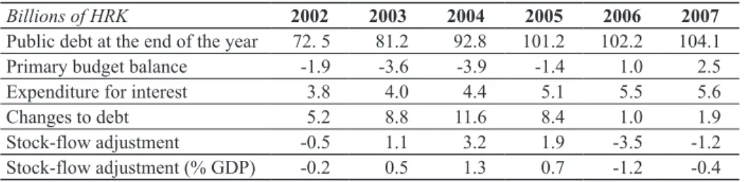
For this reason, in projections of the public debt we will use the expected values of stock-flow adjustment, based on calculated values shown in Table 5, obtained by simple alterations to the equation (13) and then division by the GDP.

Table 5 Stock-flow adjustment 2002-2007

Billions of HRK 2002 2003 2004 2005 2006 2007

Public debt at the end of the year 72. 5 81.2 92.8 101.2 102.2 104.1 Primary budget balance -1.9 -3.6 -3.9 -1.4 1.0 2.5 Expenditure for interest 3.8 4.0 4.4 5.1 5.5 5.6

Changes to debt 5.2 8.8 11.6 8.4 1.0 1.9

Stock-flow adjustment -0.5 1.1 3.2 1.9 -3.5 -1.2 Stock-flow adjustment (% GDP) -0.2 0.5 1.3 0.7 -1.2 -0.4

Source: Ministry of Finance; author’s calculation

Although we also know the figures for 2008, we did not take them into consideration as Croatian Motorways was excluded from the general government and adjustment of the debt gives a much higher value than it should be.

4.1 Modelling trends of stock-flow adjustment

In different years different stock-flow adjustment values are realized, and these are mainly small, but still not insignificant ratios in the GDP, whether positive or negative. For this reason it makes sense to assume that stock-flow adjustments have standard nor-mal distribution. Indeed, the KS test confirmed our assumption, so at a level of signifi-cance up to 96.7% we cannot reject the hypothesis that the figures arise from a standard normal distribution.

(16)

we come to a important and interesting conclusion, which is that there is a connection be-tween the movements of these two variables. A graphical presentation of the movements in the primary budget balance and the stock-flow adjustment is shown in Graph 7.

Graph 7 Primary budget balance and stock-flow adjustment (% GDP), 2002-07.

1,5

1,0

0,5

0

-0,5

-1,0

-1,5

-2,0

2002. 2003. 2004. 2005. 2006. 2007.

adjustment of flow debt primary budget balance

In years in which a primary deficit is realized, the stock-flow adjustment is mainly positive, but also the reverse. This makes sense since the stock-flow adjustment depends on many external variables, and is mainly linked with market trends. Therefore, we can assume that in difficult years, apart from realization of a negative budget balance, a large number of debts are also activated (e.g. guarantees), the domestic currency is liable to de-preciate in relation to foreign currency, the state is forced by injections of capital to help some businesses important for economic development, which have found themselves in difficulties etc. This all leads to a growth in stock-flow adjustment and therefore the pub-lic debt. We also notice a similar connection between those two variables in EU-27 mem-ber countries, so for example in 2008 in comparison to the previous year the budget def-icit rose by 1.5 percentage points, and the stock-flow adjustment by as much as 2.9 per-centage points (Eurostat, 2009c).

Therefore we assume that the ratio of the stock-flow adjustment can be estimated from the ratio of the primary budget balance in the GDP. By analysing those two varia-bles we obtain the regression line given in the following expression:

(-0.87*) (-2.27) x

W = -0 2815 0 6848, – , ⋅b e

(

)

( )

bp+e 6848

27

⋅

(

)

( ) (14)

Where bp

is the vector of primary deficit realized in the period from 2002-2007 and

(17)

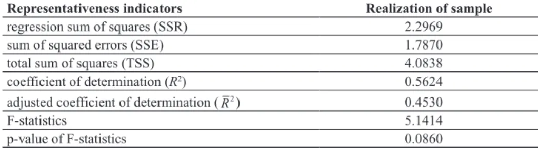
the level of significance of 76%. The indicators of representativeness of this model are shown in Table 6.

Table 6 Indicators of representativeness of the model to describe the trends in stock-flow adjustment

Representativeness indicators Realization of sample

regression sum of squares (SSR) 2.2969 sum of squared errors (SSE) 1.7870

total sum of squares (TSS) 4.0838

coefficient of determination (R2₎ _0.5624 adjusted coefficient of determination (R2₎ _0.4530

F-statistics 5.1414

p-value of F-statistics 0.0860

The coefficient of determination and the p-value of F-statistics show the satisfactory representativeness of the model described by formula (14).

Under the assumption that this relationship between the primary deficit and the stock-flow adjustment will remain in future, we can assess the effect of the crisis on the move-ments of the public debt. We will now use an adjusted version of equation (13):

d r

gd b s

t t t

p t

= +

+ +

1

1 −1– (15)

Where the lower case letters indicate the ratio in the GDP, r the real interest rate on the public debt and g the real growth rate of the GDP. So, we will calculate the ratio of the public debt in the GDP recursively, with the estimated value of the other parameters. Since

bt p_and_s

t are, according to the assumption, the realization of two dependent random

var-iables (Xt and Wt), we can form a random variable that connects them as follows:

Zt = -Xt +Wt (16)

The random variable Z_tactually signifies the change in the ratio of the public debt in the GDP due to the realization of the value of the primary deficit and the stock-flow ad-justment. Since the mathematical expectation of the random variable is a linear function-al, the following applies10_:

EZt =E

[

-Xt +Wt

]

= -EXt+EWt (17)

Which means that we can express the expected value of change in year t + k, with combination with equations (10) and (14), as:

(18)

x

EEZt k++= -0 2815 1 6848, – , 6848⋅⋅(f t( +)k) (18)

On the other hand, the variance cannot be expressed as the sum of variances, since the variable Xt and Wt are dependent, but the expression applies:

VarZt =Var X(- t+Wt)=VarXt +VarWt – 2– 2⋅xC⋅Cov X W( t, t) (19)

Which finally leads to:

VarZt k+ =2 8384, (k+1)+1 (20)

The variances of the random variables Zt + k grow with all further projections, which

leads to increasing uncertainty in the estimate.

4.2 Projection of the real growth of the GDP and real interest rates

In projections of the primary deficit and stock-flow adjustment, we rely on the prob-ability frameworks, or we consider the expected movements of variables with deviations included. This is logical in view of the fact that they are variables which have a tendency towards major deviations from the expected values. Also, every projection further into the future carries more uncertainty so there the expected deviation is greater. On the other hand, in the projections of the growth rate of the real GDP and real interest rates we as-sume that it is sufficient to follow the framework of the expected values for several rea-sons. The first reason for introducing this assumption is already visible in formula (15), as small deviations from the estimated values (for example one percentage point) have a very small multiplicative effect on last year’s ratio of the public debt. Second, and per-haps more important, is the fact that those deviations modelled stochastically make it much more difficult to calculate confidence intervals for movements of the public debt, whilst the quality of the estimate of reliability gains practically nothing. For this reason we see these variables as exogenous and without analysis of possible deviations which may occur for countless different reasons.

As with the primary deficit, the growth rate of the real GDP in the first years of the crisis also records lower (and even negative) values, but after the first initial years of the crisis there is a gradual recovery. In this mid-term projection, 2009 is assessed on the basis of the available information given above, whilst for the future projections a simple func-tion will be used, defined by the following expression:

g_{t k} g gt k

+ = + −

+ 2

3 1

(19)

to the average, and that that growth will gradually increase to the level of average growth. Table 7 shows the projection of real growth of the GDP in the period up to 2013.

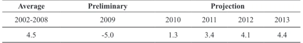
Table 7 Projections of real growth of GDP (%), 2002-13

Average Preliminary Projection

2002-2008 2009 2010 2011 2012 2013

4.5 -5.0 1.3 3.4 4.1 4.4

According to the assumption of the trend of real GDP growth described by formula (21) up to 2013, the trend of growth recovers almost completely and returns to a level close to the pre-crisis average. Moreover, a projection created in this way shows some op-timal development and gradual improvement of the situation in the economy, which is why we have reasons to believe that the chosen function is good enough for this model.

We will project the average real interest rate on the public debt under the assumption that it follows the average values realized in the period from 2002 to 2007. We are not taking into account the average in 2008 as that year Croatian Motorways (HAC) was ex-cluded from the general government, and the inflation rate measured by the change in the GDP deflator was 6.4%, which is a large rise in relation to the average growth of the GDP deflator of 3.7% in the period from 2002-2007. The average real interest rate in the peri-od in question was 1.8%, and future projections will be founded on that figure, although it is completely realistic to expect that the real interest rate on the public debt will fluctu-ate at levels higher than the average in 2002-2007. But as we have already mentioned this does not have a major influence in formula (15) on the movements of the public debt.

4.3 Projection of the public debt

In the previous sections a detailed description was given of the analytical framework which will be used to project the public debt. Since recursive projections into the increas-ingly distant future are subject to increasing deviation, apart from the expected projections, standard deviations will also be expressed. This is extremely important since the projec-tions are based on a stochastically modelled approach, in which the effect of fiscal poli-cies in the future period is not included explicitly but is formed as a normal deviation.

(20)

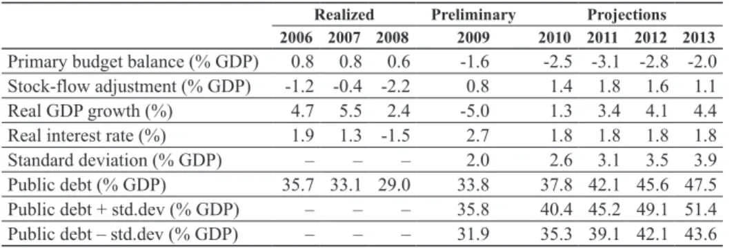
Table 8 Realized values and projections of the public debt, 2006-2013

Realized Preliminary Projections

2006 2007 2008 2009 2010 2011 2012 2013

Primary budget balance (% GDP) 0.8 0.8 0.6 -1.6 -2.5 -3.1 -2.8 -2.0 Stock-flow adjustment (% GDP) -1.2 -0.4 -2.2 0.8 1.4 1.8 1.6 1.1 Real GDP growth (%) 4.7 5.5 2.4 -5.0 1.3 3.4 4.1 4.4 Real interest rate (%) 1.9 1.3 -1.5 2.7 1.8 1.8 1.8 1.8 Standard deviation (% GDP) – – – 2.0 2.6 3.1 3.5 3.9 Public debt (% GDP) 35.7 33.1 29.0 33.8 37.8 42.1 45.6 47.5 Public debt + std.dev (% GDP) – – – 35.8 40.4 45.2 49.1 51.4 Public debt – std.dev (% GDP) – – – 31.9 35.3 39.1 42.1 43.6

In the case of the basic mid-term projection, as in the case of the mid-term projection increased by one standard deviation, the public debt meets the Maastricht criteria of con-vergence and does not exceed the limit of 60% of the GDP. Graph 8 shows the expected movements of the ratio of the public debt in the GDP and the confidence interval for that expected value.

Graph 8 Projection of the public debt and confidence intervals (% GDP), 2006-13

2006 2007 2008 2009 2010 2011 2012 2013

99% confidence interval 95% confidence interval 90% confidence interval public debt projection 60

55

50

45

40

35

30

25

(21)

Based on this projection the public debt records a constant rise, but by 2013 even the upper limit of the 99 percent confidence interval does not exceed 60% of the GDP. If we take this prescribed limit as a condition of sustainability, we can conclude with a proba-bility of 99% that the ratio of the public debt in the GDP will be sustainable up to 2013. The basic projection foresees that in 2013 the ratio of the public debt could be at around 47% but there is an obvious trend of slower growth, so after 2013 the public debt could reverse the trend and begin to decrease.

Conclusion 5

The basic projection of the trend of movements of the primary deficit for Croatia, ob-tained by adjustment of the trends of movement in EU-12 member countries, under the assumption that the macroeconomic variables are exogenous, shows significant growth of the revenue shortfall in relation to expenditure in the first three years of the crisis. After this the situation gradually improves, but even after five years the primary deficit does not reach the level of the pre-crisis years. The cause of this unfavourable trend is to be found in the stagnation of growth or even the fall in budget revenues on the one hand, and the strong growth of expenditure on the other. Since all the variables are seen as ratios of the GDP, it is important to note that in the first and sometimes in the second crisis year the GDP achieves a negative growth rate, and even after the beginning of the recovery of eco-nomic growth, although positive, it is much lower than the average of the pre-crisis peri-od. This results in an unfavourable trend of movements of the primary deficit.

The variable of the primary deficit, although it has a significant role in the formation of the changes of the public debt, is not sufficient to quantify it completely, and so addi-tional variables were used in the analysis: stock-flow adjustment, the growth rate of the real GDP and the real interest rate. On analysis the stock-flow adjustment, a negative cor-relation was found with the primary deficit, which means that those variables can be linked in the model. Basic macroeconomic variables are considered as exogenous variables, with-out consideration of the interaction of macroeconomic variables in Croatia and between other countries and Croatia. Moreover, all possible reactions of economic policies were also excluded. Instead, by formation of confidence intervals of the estimate, all potential sources of uncertainty were included, regardless of their origin.

The results obtained indicate a worrying growth of the public debt. The problem is mainly found precisely in the negative correlation between the stock-flow adjustment and the primary budget balance, and in difficult years, in which the primary deficit grows, the stock-flow adjustment also grows, which directly implies the growth of the public debt. However, in this mid-term projection up to 2013, the public debt meets the condition of sustainability and even at the upper limit of the 99 percent confidence interval it does not exceed the limit of 60% of the GDP, whereby we can confirm the main hypothesis of the sustainability of the public debt up to 2013.

(22)

develop-Financial Theory and Practice 33 (3) 273-298 (2009)

ment of the Croatian economy, which indicates the necessity of quality management of the public debt in the future. This research may serve as a small warning sign about the possible negative implications of poorly managed fiscal policies.

One of the major failings of this analysis is the too short series of comparable data. Comparison of data on a quarterly or even a monthly level would give a longer time se-ries which would certainly give better quality results. But since data on a quarterly level do not exist for all the variables used in this analysis, or even if they do exist they are not comparable, it was not possible to conduct that kind of analysis. Moreover, in this study the movements of the primary deficit and stock-flow adjustment are modelled mainly sta-tistically, and the potential shocks from macroeconomic variables are not included. Fur-ther research should certainly included a more detailed analysis of macroeconomic vari-ables, as well as a whole series of possible reactions of economic policies.

Appendix 6

Properties of mathematical expectation

Let Xi, i = 1,..., n be the random variables, and αi∈. Then the following is true:

E E i n i i i n i i X X = =

∑

⎡ ⎣ ⎢ ⎢ ⎤ ⎦ ⎥ ⎥ 1 1

α = α (d1)

In other words, the mathematical expectation is a linear functional.

Under the condition that all Xi, i = 1,..., n are independent, the following is true:

E E i n i i i n i i X X = =

∏

⎡ ⎣ ⎢ ⎢ ⎤ ⎦ ⎥ ⎥ 1 1

α = α (d2)

Variance and covariance

Let Xi, i = 1,..., n be random variables, and α βi, i∈. Then the following is true:

Var X Var X i

n

i i i i

n

i i

i j

= = <

∑

(

+

)

∑

⎡ ⎣ ⎢ ⎢ ⎤ ⎦ ⎥ ⎥

( )

1 1 2 2

α β = α + αα α_i _jCov X X( _i, _j) _(d3)

where VarXi signifies the variance of the random variable Xi, i = 1,..., n, Cov(Xi, Xj) and

the covariance of the random variables and Xi i Xj.

Under the condition that all Xi, i = 1,..., n are independent, the following is specially true:

Var X Var X i

n

i i i i n i i = =

∑

(

)

∑

⎡ ⎣ ⎢ ⎢ ⎤ ⎦ ⎥ ⎥

( )

1 1 2

α +β = α (d4)

In general the covariance may be expressed as:

(23)

Applications in the study

We recall the formulas (8) and (14):

Xt k f t k

i t t k i + = + ( )

∑

=  + + ε (8)

x

WWt k++=−−0 2815 0 6848, – , 6848⋅X⋅X+t k+ +εε+t k+ (14)

From (8) it is easy to see (10):

EXt k+ = f t( +k) (d6)

VarXt k+ =k+ 1 (d7)

On the other hand, (14) may be written as:

x

Wt k+

= + ⋅⎛ ( ) ⎝ ⎜⎜ ⎜ ⎞ ⎠ ⎟⎟⎟⎟

∑

= -0 2815 0 6848, – , f t k ε ε+ i t t k i + = + ⋅⎛ ( ) ⎝ ⎜⎜ ⎜ ⎞ ⎠ ⎟⎟⎟⎟

∑

+ +

6848 ε ++εt k+ (14)

From which, from the example of the expressions (d1) and (d4), the expressions fol-low:

x

EEWt k++= -0 2815 0 6848, – , 6848⋅⋅(f t( +)k) (d8)

x

VarWt k+ Var

= + + ⋅ ⎛ ⎝ ⎜⎜ ⎜ ⎞ ⎠ ⎟⎟⎟⎟

∑

= -0 6848, ε Varε ( )

i t t k

i t k

+ = + + ⋅ ⎛ ⎝ ⎜⎜ ⎜ ⎞ ⎠ ⎟⎟⎟⎟

∑

+

6848 ε ε ==0 4689, (k+1)+1 (d9) The change in the debt due to the realization of the primary deficit and the stock-flow adjustment is defined by formula (16):

Zt = -Xt +Wt (16)

By application of the property of (d1) to the expression (16) we obtain:

EZ_t =E

[

-X_t +W_t

]

= -EX_t +EW_t (17) Or by inclusion of (d6) and (d8):

x

EEZt k++= -0 2815 1 6848, – , 6848⋅⋅(f t( +k)) (18)

Applying the expression (d3) we obtain an expression for the variance:

(19) From this expression we have the well-known VarXt and VarWt, and we only need to

express Cov(Xt, Wt). For this we will use formula (d5):

(24)

For the sake of simplicity we will calculate each member of the expression (d5’) sep-arately using the formula above:

x

E

[

Xt k+Wt k+

]

=E⎡⎣⎢Xt k+

(

-0 2815 0 6848, – , ⋅ + ε+

)

⎤⎦⎦⎥

⎡⎣ ⎤⎦ ⋅

[

]

+ + + +

E E E E ε

E + E⎡⎣ + ⎤⎦

E

[

+ +

]

E⎡⎣⎢ +

(

⋅ + ε+

)

⎤⎦⎦⎥

⎡⎣ ⎤⎦ ⋅

[

]

+ + + +

E E E Eε

=

= -0 2815 0 6848 2

, EXt k+ – , E⎡⎣Xt k+ ⎤⎦

E

[

+ +

]

E⎡⎣⎢ +

(

⋅ + ε+

)

⎤⎦⎦⎥

⎡⎣ ⎤⎦ ⋅

[

]

+ + + +

= -0 2815 0 6848 2 +

, EXt k– , E Xt k EXt k E ε

E + E⎡⎣ + ⎤⎦

E

[

+ +

]

E⎡⎣⎢ +

(

⋅ + ε+

)

⎤⎦⎦⎥

⎡⎣ ⎤⎦ ⋅

[

]

+ + + +

E E E E εt k

E + E⎡⎣ + ⎤⎦

E

[

+ +

]

E⎡⎣⎢ +

(

6848⋅X_{t k}+ +ε_{t k}+

)

⎤⎦⎦⎥

⎡⎣ ⎤⎦ ⋅

[

]

+ + + +

E E E E ε

E + E⎡⎣ + ⎤⎦

x

Since the following is true:

VarXt k+ =E⎡⎣Xt k2+ ⎤⎦

(

E

[

Xt k+

]

)

⋅E⎡⎣ + ⎤⎦= +

2

– Xt k VarXt

(

E

[

+

]

)

+ =E⎡⎣ + ⎤⎦

(

E

[

+

]

)

⋅E⎡⎣ + ⎤⎦= +

2 ₂

kk+

(

E

[

Xt k+

]

)

2

x

By including in the upper expressions for expectation Xt + k Xt + k we obtain:

E

[

+ +

]

E + ⋅ + ⋅ EE

f t k k f t

+

[

]

(

)

+

( ) ( + ) +

0 2815 0 6848 1 0 6848

= - , – , – , ⎡_⎣ ( kk)⎤_⎦2

E

[

Xt k+Wt k+

]

= -0 2815, EXt k+ –0 6848, ⋅V + – ⋅

(

EE

[

+

]

)

+

( ) ( + ) ⎡_⎣ ( + )⎤_⎦

E

[

+ +

]

E + – 6848⋅VarXt k+ –0 6848, ⋅

(

EE

[

+

]

)

+

( ) ( + ) ⎡_⎣ ( + )⎤_⎦

E

[

+ +

]

E + ⋅ + 6848⋅

(

EE

[

Xt k+

]

)

+ ( ) ( + ) + 2 ( ) ⎡ ⎣ ⎤⎦ x x

EXt k+ EWt k+ = f t( +k)⋅

(

⋅ ( )

)

( ) ⎡_⎣ ( )⎤_⎦

E + E + ( )⋅

(

-0 2815 0 6848, – , ⋅ ( )

)

( ) ⎡_⎣ ( )⎤_⎦

E +E + ( )⋅

(

6848⋅f t( +k)

)

=

( ) ⎡_⎣ ( )⎤_⎦

E + E + ( )⋅

(

⋅ ( )

)

= -0 2, 8815f t( +k)–0 6848, ⎡_⎣f t( +k)⎤_⎦2.

x x

The last two expressions obtained give:

Cov X

(

t k+ ,Wt k+

)

= -0 6848, (k+1) (d5’’)

Finally by combining expressions (19), (d7), (d9) and (d5’’) we obtain the expression for variance from Zt+k:

x

VarZt k++=k+ +1 0 4689, (k(+1))+ ++ +1 2 02 0 6848⋅⋅ , ((k+1))=2 8384, ((k++)1)+1 (20)

LITERATURE

---, 2009a. Hrvatska ušla u recesiju [online]. Available from: [http://www.bankamaga-zine.hr/Naslovnica/Vijesti/Hrvatska/tabid/102/View/Details/ItemID/47321/Default.aspx]. ---, 2009b. Vodeći ekonomisti očekuju pad BDP-a od 5% [online]. Available from: [http://www.bankamagazine.hr/Naslovnica/Vijesti/Hrvatska/tabid/102/View/Details/Item-ID/53045/ttl/Vodeci-ekonomisti-ocekuju-pad-BDP-a-od-5-posto/Default.aspx].

Babić, A. i sur., 2003. “Dinamička analiza održivosti javnog i vanjskog duga Hrvat-ske” [online]. Privredna kretanja i ekonomska politika, br. 97. Available from: [http://www. eizg.hr/AdminLite/FCKeditor/UserFiles/File/pkiep97-babi-krznar-nesti-valjek.pdf].

(25)

DZS, 2009a. Indeksi potrošačkih cijena u srpnju 2009. - priopćenje [online]. Avail-able from: [http://www.dzs.hr/Hrv/publication/2009/13-1-1_7h2009.htm].

DZS, 2009b. Procjena tromjesečnog obračuna bruto domaćeg proizvoda za prvo tromjesečje 2009. - priopćenje [online]. Available from: [http://www.dzs.hr/Hrv/ publication/2009/12-1-1_1h2009.htm].

DZS, 2009c. Godišnji bruto domaći proizvod od 1995. do 2005. - priopćenje [online]. Available from: [http://www.dzs.hr/Hrv/publication/2009/12-1-3_1h2009.htm].

DZS. Mjesečno statističko izvješće [online]. Available from: [http://www.dzs.hr/Hrv/ publication/msi.htm].

DZS. Statistički ljetopis [online]. Available from: [http://www.dzs.hr/Hrv/publication/ stat_year.htm].

Euromonitor International, 2009. The global financial crisis: recession bites into Western Europe [online]. Available from: [http://www.euromonitor.com/The_global_fi-nancial_crisis_recession_bites_into_Western_Europe].

European Communities, 2002. ESA95 manual on government deficit and debt [on-line]. Luxembourg: Office for Official Publications of the European Communities. Available from: [http://epp.eurostat.ec.europa.eu/cache/ITY_SDDS/Annexes/gov_dd_sm1_an4.pdf]. European Communities, 2009. “Public finances in EMU” [online]. European Econ-omy, No. 5. Available from: [http://ec.europa.eu/economy_finance/publications/publica-tion15390_en.pdf].

Eurostat, 2009a. Annual average inflation rate - Annual average rate of change in Harmonized Indices of Consumer Prices [online]. Available from: [http://epp.eurostat. ec.europa.eu/tgm/table.do?tab=table&language=en&pcode=tsieb060&tableSelection=1 &footnotes=yes&labeling=labels&plugin=1].

Eurostat, 2009b. GDP per capita in PPS [online]. Available from: [http://epp.euro-stat.ec.europa.eu/tgm/table.do?tab=table&init=1&plugin=1&language=en&pcode=tsie b010].

Eurostat, 2009c. Stock-flow adjustment (SFA) for the Member States, the euro area and the EU27 for the period 2005-2008, as reported in the April 2009 EDP notification

[online]. Available from: [http://epp.eurostat.ec.europa.eu/cache/ITY_PUBLIC/STOCK_ FLOW_2009_1/EN/STOCK_FLOW_2009_1-EN.PDF].

Hiebert, P and Rostagno, M., 2000. “Close to Balance or in Surplus”: A Methodol-ogy to Calculate Fiscal Benchmarks“ [online]. Fiscal Sustainability, 95-133. Banca d’Italia, Research Department Public Finance Workshop. Available from: [http://www.bancadita-lia.it/studiricerche/convegni/atti/fiscal_sust/i/095-134_hiebert_and_rostagno.pdf].

IMF, 2003. Sustainability Assessments - Review of Application and Methodological Refinements [online]. Prepared by the Policy Development and Review Department. Avail-able from: [http://www.imf.org/external/np/pdr/sustain/2003/061003.pdf].

(26)

Mihaljek, D., 2003. “Analiza održivosti javnog i vanjskog duga Hrvatske pomoću standardnih financijskih pokazatelja” [online]. Privredna kretanja i ekonomska politika, br. 97. Available from: [http://www.eizg.hr/AdminLite/FCKeditor/UserFiles/File/pkiep97-mihaljek.pdf].

Ministarstvo financija, 2009a. Konsolidirana opća država [online]. Available from: [http://www.mfin.hr/adminmax/docs/Opca_drzava_-_sijecanj_-_lipanj_2009.xls].

Ministarstvo financija, 2009b. Mjesečni statistički prikaz Ministarstva financija, br. 160

[online]. Available from: [http://www.mfin.hr/adminmax/docs/Statistika_hrvatski_160.pdf]. Ministarstvo financija, 2009c. Rebalans proračuna 2009. [online]. Available from: [http://www.mfin.hr/adminmax/docs/Obrazlozenje_Rebalans3_2009.pdf].

Reinhart, C. M. and Rogoff, K. S. , 2008. “Banking crises: an equal opportunity menace” [online]. NBER Working Paper, No. 14587. Available from: [http://www.nber. org/papers/w14587.pdf].

Švaljek, S., 2007. “Javni dug” u: K. Ott, ur. Javne financije u Hrvatskoj. Zagreb: In-stitut za javne financije, 75-90.