www.atmos-chem-phys.net/10/4013/2010/ doi:10.5194/acp-10-4013-2010
© Author(s) 2010. CC Attribution 3.0 License.
Chemistry
and Physics
Corrigendum to
“A novel downscaling technique for the linkage of global and
regional air quality modeling” published in Atmos. Chem. Phys.,
9, 9169–9185, 2009
Y. F. Lam and J. S. Fu
Department of Civil and Environmental Engineering, University of Tennessee, Knoxville, TN, USA
We have discovered that the previously published paper was not the latest version of the manuscript we intended to use. Some corrections made during the second ACPD reviewing process were not incorporated in the text. As a result, the figure numbers (i.e., figure number below the graph) were not referenced correctly in the manuscript. Therefore, we have decided to re-publish this paper as a corrigendum.
Abstract. Recently, downscaling global atmospheric model outputs (GCTM) for the USEPA Community Multiscale Air Quality (CMAQ) Initial (IC) and Boundary Conditions (BC) have become practical because of the rapid growth of com-putational technologies that allow global simulations to be completed within a reasonable time. The traditional method of generating IC/BC by profile data has lost its advocates due to the weakness of the limited horizontal and vertical variations found on the gridded boundary layers. Theoret-ically, high quality GCTM IC/BC should yield a better re-sult in CMAQ. Unfortunately, several researchers have found that the outputs from GCTM IC/BC are not necessarily better than profile IC/BC due to the excessive transport of O3aloft in GCTM IC/BC. In this paper, we intend to investigate the effects of using profile IC/BC and global atmospheric model data. In addition, we are suggesting a novel approach to re-solve the existing issue in downscaling.
In the study, we utilized the GEOS-Chem model out-puts to generate time-varied and layer-varied IC/BC for year 2002 with the implementation of tropopause determin-ing algorithm in the downscaldetermin-ing process (i.e., based on chemical (O3) tropopause definition). The comparison
be-Correspondence to:J. S. Fu ([email protected])
tween the implemented tropopause approach and the profile IC/BC approach is performed to demonstrate improvement of considering tropopause. It is observed that without us-ing tropopause information in the downscalus-ing process, un-realistic O3concentrations are created at the upper layers of IC/BC. This phenomenon has caused over-prediction of sur-face O3in CMAQ. In addition, the amount of over-prediction is greatly affected by temperature and latitudinal location of the study domain. With the implementation of the al-gorithm, we have successfully resolved the incompatibility issues in the vertical layer structure between global and re-gional chemistry models to yield better surface O3 predic-tions than profile IC/BC for both summer and winter condi-tions. At the same time, it improved the vertical O3 distri-bution of CMAQ outputs. It is strongly recommended that the tropopause information should be incorporated into any two-way coupled global and regional models, where the tro-pospheric regional model is used, to solve the vertical incom-patibility that exists between global and regional models.
1 Introduction
et al., 2007) and enhancement of background pollutant con-centrations emerged (Vingarzan, 2004; Ordonez et al., 2007; Fiore et al., 2003). Various studies suggested that utilizing dynamic global chemical transport model (CTM) outputs as the BCs for the regional air quality model would be the best option for capturing the temporal variation and spatial distri-butions of the tracer species (Fu et al., 2008; Byun et al., 2004; Morris et al., 2006; Tang et al., 2007). For exam-ple, Song et al., (2008) applied the interpolated values from a global chemical model, RAQMS, as the lateral BCs for the regional air quality model, CMAQ and evaluated simulated CMAQ results with ozone soundings. Simulations were per-formed on the standard CMAQ seasonal varied profile BCs and dynamic BCs from RAQMS. The results demonstrated that the scenario with dynamic BCs performed better than the scenario with profile BCs in terms of the prediction of vertical ozone profile.
The quality of BCs depends on the vertical, horizontal, and temporal resolutions of global CTM outputs. The latitudi-nal location and seasolatitudi-nal variation are also playing an im-portant role, which defines the tropopause height that influ-ences the vertical interpolation process between global and regional models. (Bethan et al., 1996; Stohl et al., 2003) In the MICS-Asia project, high concentrations of ozone (i.e., 500 ppbv) have been observed in CMAQ BCs when the re-gional model’s layers reach above or beyond the tropopause height during the vertical interpolation process. (Fu et al., 2008) This high ozone aloft in BCs has created problems for the regional tropospheric model (such as CMAQ) since it does not have a stratospheric component or stratosphere-troposphere exchange mechanism. As a result, unrealisti-cally high ozone concentrations were observed at the sur-face layer during the regional CTM simulations. Tang et al. (2009) studied various CTM lateral BCs from MOZART-NCAR, MOZART-GFDL, and RAQMS. They observed that CTM BCs have induced a high concentration of ozone in the upper troposphere in CMAQ; this high ozone aloft quickly mixed down to the surface resulting in an overestimation of surface ozone. Mathur et al., suggested that the overesti-mation of O3 might also be partially contributed by the in-adequate representation of free tropospheric mixing due to the selection of a coarse vertical resolution (Mathur et al., 2008; Tang et al., 2009) Since the rate of vertical trans-port of flux is highly sensitive to temperature and moisture-induced buoyancies, correctly representing deep convection or flux entrainment at the unstable layer in the meteorological model becomes critical to modeling ozone vertical mixing. It should be noted that the single PBL scheme in the meteoro-logical model is not sufficient to simulate the correct vertical layer structure on the broad aspect of environmental condi-tions (i.e., terrain elevation and PBL height) in the existing domain. As a result, it introduces uncertainties and errors to the process of determining vertical transport of O3in the air quality model (Zangl et al., 2008; Perez et al., 2006) For the downscaling problem, Tang et al. (2009) has commented
that using outputs of the global CTM (GCTM) as BCs may not necessarily be better than the standard profile-BC, which highly depends on location and time. The quick downward mixing in CMAQ has caused an erroneous prediction of sur-face ozone when both tropospheric and stratospheric ozone are included in the CTM BCs. (Al-Saadi et al., 2007; Tang et al., 2007; Tang et al., 2009) Therefore, correctly defin-ing tropopause height for separatdefin-ing troposphere and strato-sphere becomes crucial to the prevention of stratospheric in-fluence during the vertical interpolation process for CMAQ and other regional CTMs simulation.
The tropopause is defined as the boundary/transitional layer between the troposphere and the stratosphere, which separates by distinct physical regimes in the atmosphere. The height of tropopause ranges from 6 km to 18 km depending on seasons and locations (Stohl et al., 2003). In the USA, the typical tropopause height in summer ranges from 12 km to 16 km, but drops to 8 km to 12 km in winter (Newchurch et al., 2003). Various techniques were developed for identi-fying the altitude of tropopause, which are based on temper-ature gradient, potential vorticity (PV), and ozone gradient. In meteorological studies, such as satellite and sonde data analysis, temperature gradient method, also referred to as the thermal tropopause method, is the most commonly used tech-nique, which searches the lowest altitude where the temper-ature lapse rate decreased to less than 2◦K/km for the next 2 km and defines that as tropopause. (WMO, 1986) In cli-mate modeling, PV technique, referred to as dynamic tech-nique, is often applied to define tropopause. PV is a verti-cal momentum up drift parameter and is expressed by PV unit (PVU). The threshold value of the tropopause lies be-tween±1.6 to 3.5 PVU depending on the location on the globe (Hoinka, 1997), Recently, in an attempt to improve the regional model (i.e., the pure tropospheric model), CMAQ (to simulate ozone at the lower stratosphere) was performed using Potential Vorticity relationship. Location-independent correlation between PVU with ozone concentrations was ap-plied to correct the near/above-tropopause ozone concentra-tions in CMAQ. The fundamental disadvantage of using such technique is the implementation of a single correlation pro-file (i.e.,R2= 0.7) to represent the entire study domain (i.e., the Continental USA). It shows that a slight shift of PV value in the profile could result in a big change of ozone concen-tration, up to 100 ppbv. In addition, this profile may not be applicable for all locations in the domain due to the limited amount of data in the literature (Mathur et al., 2008). In GCTM downscaling, the ozone gradient technique, referred to as chemical tropopause or ozone tropopause, is more ap-propriate for defining tropopause since we have observed the stratospheric level of ozone (i.e., about 300 ppbv) at the level of thermal and dynamic tropopause (Lam et al., 2008).
than the thermal and dynamic tropopause. (Bethan et al., 1996) The height of tropopause affects both the stratosphere-troposphere exchange (STE) as well as the transport of O3at upper troposphere. (Holton et al., 1995; Stohl et al., 2003) In global CTM, well-defined vertical profiles of troposphere, tropopause, and stratosphere are established for simulating STE, upper tropospheric advection, and other atmospheric processes. Collins (2003) estimated that the net O3flux from the stratosphere could contribute 10 to 15 ppbv of the over-all tropospheric ozone. (Collins et al., 2003), where Stohl (2003) has found about 10% to 20% of tropospheric ozone are originated from stratosphere (Stohl et al., 2003). The ad-vantage of employing CTM outputs as BCs gives a better rep-resentation of upper troposphere and the effect of STE can be taken into account. Although global CTM is capable of simulating tropospheric conditions, the temporal and spatial resolutions may not be sufficient to represent the daily and monthly variability of surface conditions since the monthly chemical profile of budget is used. Several researchers have demonstrated the outputs of global CTM can be used in the area of surface background conditions and trends (Park et al., 2006; Fiore et al., 2003). However, it also indicated that the global CTM is inadequate to predict the peak magnitude of O3at the surface since it is not intended to describe de-tailed surface flux condition at a high temporal and spatial resolution. Therefore, the regional air quality model remains indispensable for simulating the surface O3conditions.
In this study, we have developed a linking tool to pro-vide lateral BCs of the USEPA Community Multiscale Air Quality (CMAQ) model with the outputs from GEOS-Chem (Byun and Schere, 2006; Lam et al., 2008; Li et al., 2005). One full year of GEOS-Chem data in 2002 are analyzed and summarized to explore the seasonal variations of O3 ver-tical profiles and tropopause heights in global CTM with available ozonesonde data in the USA are used to verify the performance of the GEOS-Chem model. Evaluations are conducted to measure the potential impact of changing tropopause height to the performance of the interpolated BCs toward the regional CTM. A new algorithm, “tropopause-determining algorithm”, which is based on chemical (O3) tropopause definition, is proposed for the vertical interpola-tion process during downscaling to remove stratospheric ef-fects from the global CTM toward the regional CTM. Verifi-cations of the new algorithm are performed using three sets of CMAQ simulations, which are (1) the static lateral BCs from predefined profile is used as an experimental control for GEOS-Chem data inputs; (2) standard dynamic lateral BCs from GEOS-Chem using original vertical interpolation; and (3) the modified dynamic lateral BCs from GEOS-Chem, and is intended to show the improvement of the proposed idea using the observation data from ozonesonde and CASTNET. Moreover, it demonstrates the necessity of filtering the tro-pospheric portion of global GMC outputs for the inputs in regional air quality modeling.
2 Description and configuration of models used
In this study, GEOS-Chem global chemistry model output is used to provide lateral boundary conditions for the regional air quality model CMAQ, where meteorological inputs are driven by the MM5 mesoscale model. The model setups are described as follows.
3 GEOS-Chem
GEOS-Chem global chemistry model output is one of the most popular global models for generating BCs for the CMAQ regional model (Tesche et al., 2006; Morris et al., 2005; Streets et al., 2007; Tagaris et al., 2007; Eder and Yu, 2006). Many studies demonstrated that GEO-Chem is ca-pable of capturing the effects from intercontinental transport of air pollutants and increasing background concentrations. (Heald et al., 2006; Liang et al., 2007; Park et al., 2003). Please note the above referenced studies may have used dif-ferent versions of GEOS-Chem. For example, Heald used version 4.33 of GEOS-Chem, where as Liang et al. and Park et al. used version 7.02.
GEOS-Chem is a hybrid (stratospheric and tropospheric) 3-D global chemical transport model with coupled aerosol-oxidant chemistry (Park et al., 2006). It uses 3-h assimilated meteorological data such as winds, convective mass fluxes, mixed layer depths, temperature, clouds, precipitation, and surface properties from the NASA Goddard Earth Observ-ing System (GEOS-3 or GEOS-4) to simulate atmospheric transports and chemical balances. In this study, all GEOS-Chem simulations were carried out with 2◦latitude by 2.5◦
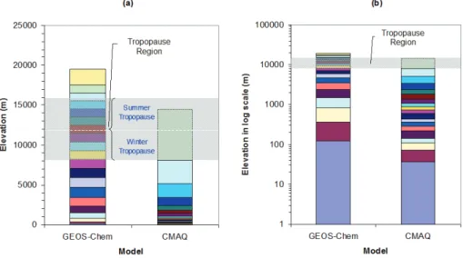
longitude (2◦×2.5◦) horizontal resolution on 48 sigma ver-tical layers. The lowest model levels are centered at ap-proximately 50, 200, 500, 1000, and 2000 m above the sur-face. Figure 1a and b show the vertical layer structure of GEOS-Chem. The grey areas indicate the height range of tropopause in summer and winter in literature. A full-year simulation was conducted for year 2002, which was initial-ized on 1 September 2001 and continued for 16 months. The first four months were used to achieve proper initialization, and the following 12 months were used as the actual simu-lation results. All simusimu-lations were conducted using version 7.02 with GEOS-3 meteorological input. Detailed discussion of GEOS-Chem of version 7.02 is available elsewhere (Park et al., 2004).
Fig. 1.Vertical layer structure comparison between GEOS-Chem and CMAQ,(a)arithmetic scale, and(b)log scale.
BOULDER (40.0N,105.25W)
0 100 200 300 400
P
res
sure (
h
P
a
)
1000 850 700 500 400 300 200 100
HUNTSVILLE (34.7N,86.61W)
2002 Ozone Concentration (ppbv) 400 300 200 100
TRINIDAD HEAD (41.05,124.15)
400 300 200 100
Ozonesonde Geos-4
Fig. 2.Yearly variability of GEOS-Chem outputs verses ozonesonde.
stratospheric ozone with the Synoz algorithm (McLinden et al., 2000), which gives us the right cross-tropopause ozone flux but no guarantee of correct ozone concentrations in the region. That is because, until recently, cross-tropopause transport of air in the GEOS fields was sometimes too fast. This is discussed for example in Bey et al., 2001; Liu et al., 2001; Fusco and Logan, 2003. Nevertheless, for this study, simple model verifications were still conducted on the GEOS-Chem outputs using available ozonesonde data in the USA (Newchurch et al., 2003) Particular interest was given to upper troposphere and tropopause regions (1000 hPa to 50 hPa), where the downscaling process could be influenced by stratospheric ozone. Figure 2 shows the yearly variabil-ity of GEOS-Chem with ozonesonde data. It is observed that 99.5% of GEOS-Chem outputs are contained within the sta-tistical range of the observation data, which gives a good in-dication of reasonable model results. For the Boulder and Huntsville sites, good model performances were found at
higher pressure when the pressure fell between 1000 hPa to 300 hPa. Consistent under-predictions were observed at the upper atmosphere when the pressures dropped below 250 hPa.
4 MM5 and CMAQ
EPA NPS
Huntsville, AL Trinidad head, CA
Boulder, CO
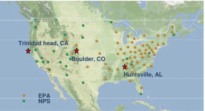
Fig. 3.The CONUS domain with observation sites marked in green or orange from CASTNET and ozonesondes in red star.
CONUS domain), which is shown in Fig. 3. In CMAQ simu-lations, three scenarios with different lateral boundary condi-tions were performed, which included profile boundary con-ditions (Profile-BC), ordinary vertical interpolated GEOS-Chem boundary conditions (ORDY-BC), and vertical inter-polated GEOS-Chem boundary conditions using the new al-gorithm (Tropo-BC). All of these simulations were config-ured with Carbon Bond IV (CB-IV) chemical mechanism with aerosol module (AERO3). The detailed configuration is also shown in Table 1.
5 Linkage methodology between GEOS-Chem and CMAQ
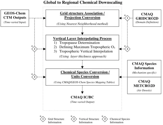
The GEOS-Chem outputs were extracted as CMAQ lat-eral boundary conditions using GEOS2CMAQ linkage tool, which involved grid structure association, horizontal/vertical interpolation, and chemical mapping processes. A summary of the systematic flowchart of the linkage methodology is shown in Fig. 4. It should be noted that most of the regional models including CMAQ do not utilize top boundary condi-tion as input. As a result, in this study, no top boundary con-dition is generated. In the linkage process, GEOS2CMAQ applied the “nearest neighbor” method to associating the latitude/longitude formatted GEOS-Chem outputs with the CMAQ Lambert Conformal gridded format. Horizontal in-terpolating process then utilized the results to interpolate the GEOS-Chem outputs into CMAQ gridded format for each vertical layer column. For Tropo-BC, a newly developed tropopause-determining algorithm, which is based on chem-ical (O3) tropopause definition, was implemented in the ver-tical interpolating process to identify the tropopause height. Moreover, it separated the troposphere from the stratosphere for each horizontal grid. Different interpolating processes were employed in the tropospheric and the stratospheric re-gions. A detailed discussion may be found in the latter sec-tion of this document. For the chemical mapping process, 38 GEOS-Chem species were transformed into 24 CB-IV
mech-Table 1.MM5 and CMAQ Model Configurations for 2002 simula-tions.
MM5 Configuration Model version 3.7
Number of sigma level 34 Number of grid 156×120 Horizontal resolution 36 km
Map projection Lambert conformal FDDA Analysis nudging Cumulus Kain-Fritsch 2 Microphysics Mix-phase Radiation RRTM PBL Pleim-Xiu LSM Pleim-Xiu LSM LULC USGS 25-Category
CMAQ Configuration Model version 4.5
Number of Layer 19 Number of grid 148×112 Horizontal resolution 36 km Horizontal advection PPM Vertical advection PPM Aerosol module AERO3 Aqueous module CB-IV
Emission VISTAS emissions (NEI 2002 G) Boundary condition I CMAQ Predefined Vertical Profile Boundary condition II 2002 GEOS-Chem
anism species of CMAQ according to the chemical defini-tions given in Appendix A. The GEOS-Chem species with the same definitions as CB-IV species were mapped directly into CMAQ; where as other species were mapped by parti-tioning and/or regrouping processes. For example, total ox-idants Oxspecies in GEOS-Chem were defined as the com-bination of O3 and NOx. Therefore, to obtain O3 concen-trations, Ox was subtracted by NOx species in the GEOS-Chem. Other species, such as paraffin carbon bond (PAR), were composed of multiple species in GEOS-Chem. Re-grouping was required to reconstruct the CB-IV correspond-ing species, which is shown as follows:
PAR=ALK4+C2H6+C3H8+ACET+MEK+ 1
2PREP (1) For chemicals that were not supported by GEOS-Chem, CMAQ predefined boundary conditions were used to main-tain the full list of CMAQ CB-IV species.
6 Tropopause determining algorithm
GEOS-Chem CTM Outputs (Time-varied Input)
Global to Regional Chemical Downscaling
Grid structure Association / Projection Conversion
(Using Nearest Neighborhood method)
Vertical Layer Interpolating Process 1) Tropopause Determination 2) Defining Maximum Tropospheric O3
3) Tropospheric Vertical Interpolation (Using layer thickness approach)
Chemical Species Conversion / Units Conversion
(Using CMAQ/GEOS-Chem Species Mapping Tables)
CMAQ IC/BC (Time-varied Output) C
2 *
C
3 *
C
1 Grid Structure 2C 3C
Information
Vertical Structure Information
Chemical Species Information * * *
CMAQ GRIDCRO2D (Domain Definition) C
1 *
C
2 *
CMAQ METCRO2D
(Air Density) CMAQ Species
Information (Mechanism specific)
Fig. 4.Systematic flowchart of global to regional chemical downscaling.
for handling the near tropopause and stratosphere interpolat-ing processes, which is essential to correct and represent the global model outputs in the regional model. We have uti-lized the chemical/ozone tropopause definition described in Bethan (1996), instead of thermal and dynamic tropopause definitions, as the basis for separating the stratosphere and the troposphere. Although thermal and dynamic tropopauses are more commonly used in determining the tropopause, we have identified that these tropopauses are inappropriate for this application because of the observed stratospheric ozone effect at the troposphere. Since the purpose of determin-ing tropopause is to exclude stratospheric pollutants con-centrations from the global model during the interpolating process, ozone tropopause is better suited for this applica-tion. Ozone tropopause is defined as the location at which an abrupt change of ozone concentration occurred. Our algo-rithm finds the ozone tropopause by finding the largest nega-tive rate of change of slope (i.e., could be neganega-tive) from the plot of elevation verses ozone concentration. In other words, we have taken the second derivative of elevation with respect to ozone concentration and found the lowest value.
HTropo(Ci)=max
Ci+1−Ci
Hi+1−Hi
−Ci−Ci−1
Hi−Hi−1
(2) where 8km<H<19km
Each rate of change of slope requires 3 data points or 2 line segments, upon which two line slopes were calculated. In the tropopause level, which is indicated by the largest negative rate of change of slope, a combination of a small concentra-tion change in the first segment with a large concentraconcentra-tion change in the second segment were obtained. Occasionally, a false tropopause was identified when an extremely small change of ozone concentration in the first segment or nega-tive change of ozone concentrations in the second segment occurred. To ensure the tropopause found by this method is a reasonable tropopause height with no stratospheric effect, we have cross checked the tropopause results with thermal tropopause heights (i.e., ozone tropopause should be lower than thermal tropopause), as well as the maximum concen-trations of ozone should exceed 300 ppbv as found in the lit-erature. (McPeters et al., 2007).
0 300 600 900 1200 1500 0
5000 10000 15000 20000 25000
E
lev
ati
o
n
(m)
GEOS-Chem CMAQ
North Bound
Win
te
r
0 100 200 300 400
GEOS-Chem CMAQ
Tropopause region
South Bound
Su
m
m
e
r
0 300 600 900 1200 1500 0
5000 10000 15000 20000 25000
E
lev
at
io
n
(m)
GEOS-Chem CMAQ
Tropopause region
0 100 200 300 400
GEOS-Chem CMAQ
Tropopause region Tropopause region
(c) (d)
(a) (b)
O3 (ppbv) O3 (ppbv)
18* 19*
18* 19* 19*
18* 19*
18*
* CMAQ iayer no. * CMAQ layer no.
* CMAQ layer no. * CMAQ layer no.
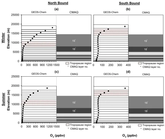
Fig. 5.Vertical ozone profiles from GEOS-Chem plotted with GEOS-Chem and CMAQ layers for both summer and winter,(a)north bound in winter,(b)south bound in winter,(c)north bound in summer, and(d)south bound in summer.
7 Results and discussion
7.1 CMAQ lateral boundary conditions
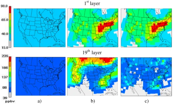
We have generated CMAQ lateral boundary conditions from every third hour GEOS-Chem output for VISTAS CMAQ simulation using GEOS2CMAQ linkage tool. Figure 5 shows the vertical ozone profiles from GEOS-Chem with CMAQ vertical layers for both summer and winter. It should be noted that the tropopause in summer is much higher than the tropopause in winter. As a result, less stratospheric ozone is included in summer than winter when the verti-cal interpolating process is performed. In Fig. 6, compar-isons of Profile-BC, ORDY-BC, and Tropo-BC for 22 June 2002 is shown on the CONUS domain. The top row rep-resents the 1st CMAQ layer (∼1000 millibars) and the bot-tom shows the top CMAQ layer (i.e., 19th layer∼140 mil-libars). These plots are intended to demonstrate the horizon-tal distribution of ozone concentrations across the CONUS domain. The Profile-BC was designed to represent the rel-atively clean air conditions for the CONUS boundaries. It enforces a pre-defined vertical profile with no temporal and spatial dependencies. In general, the surface ozone
b)
c)
a)
19
thlayer
1
stlayer
Fig. 6.Comparison of different lateral boundary conditions in 1st and 19th layers,(a)Profile-BC,(b)ORDY-BC, and(c)Tropo-BC.
235 ppbv and the Tropo-BC ozone achieves up to 160 ppbv in the CONUS domain on 22nd June. For other days in 2002, the ORDY-BC and Tropo-BC ozone reaches up to 714 ppbv and 205 ppbv, respectively. In Considine (2008), the re-ported maximum mean tropopause ozone concentration from observations in North America is about 235 ppbv based on the thermal tropopause definition. We would have expected that if Considine’s analyses used the ozone tropopause as its definition, the maximum tropopause ozone concentrations should be lower since the ozone tropopause is constantly lower than the thermal tropopause at the upper troposphere. So, the maximum ORDY-BC ozone of 714 ppbv would be too high in the troposphere and would impractically bring high ozone to surface level, where as the maximum Tropo-BC ozone of 205 ppbv has fallen within a reasonable value in the United States. It should be noted that the Considine’s data is concentration at higher latitudinal locations. With the direct proportional relationship between latitudinal location and tropopause ozone concentration, we would expect that the reported 235 ppbv should be a high end of the ozone con-centration at the tropopause in the United States.
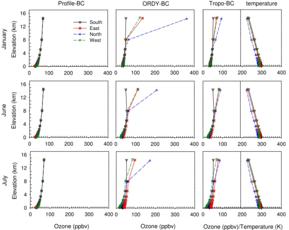
As tests of the lateral boundary conditions’ responses to the GEOS2CMAQ linkage tool, we have extracted the ver-tical profiles of various CMAQ boundary conditions for se-lected months to investigate the seasonal effects of the data. Figure 7 shows average monthly ozone vertical distribution from all four boundaries of the CONUS domain: East, West, South, and North are shown in various colors with average vertical temperature profiles for January, June, and July. Jan-uary represents the winter condition where tropopause is rel-atively low as a consequence of cold temperatures; July char-acterizes the summer condition with possible high surface
0 100 200 300 400 0
4 8 12 16
0 100 200 300 400
0 100 200 300 400
South East North West
E
levat
io
n
(km
)
J
a
nua
ry
0 100 200 300 400
0 4 8 12 16
0 100 200 300 400
0 100 200 300 400
Elev
atio
n (k
m)
Jun
e
0 100 200 300 400
0 100 200 300 400
0 4 8 12 16
Elev
atio
n (
k
m
)
Ju
ly
0 100 200 300 400
Ozone (ppbv) Ozone (ppbv) Ozone (ppbv)/Temperature (K)
Profile-BC ORDY-BC Tropo-BC temperature
Fig. 7.Monthly vertical distribution of ozone from CMAQ BCs: South (black line), East (Red line), North (blue line), and West (green line) of CONUS domain in January, June and July with temperature profiles for Profile-BC (left), ORDY-BC (middle) and Tropo-BC (right).
In addition to the seasonal effect, latitudinal effect is also observed in Fig. 7, where South bound (i.e., downward tri-angle in black) has the lowest concentration and the North bound (i.e., upward triangle in blue) exhibits the highest con-centration at the upper CMAQ layers (top two layers) on both ORDY-BC and Tropo-BC. The latitudinal effect is mainly in-duced by the temperature differences at troposphere on dif-ferent boundaries. The vertical temperature profile in CMAQ on the right shows a decrease in temperature with increase in elevation; no temperature inversion is observed. This in-dicates all CMAQ layers have fallen within the troposphere because it illustrates a tropospheric laps rate pattern.
7.2 CMAQ outputs
The CMAQ model was used to simulate the surface ozone concentrations in 36 km CONUS domain using Profile-BC, ORDY-BC and Tropo-BC with VISTAS emissions inven-tories (Morris et al., 2006). Figure 8 shows the CMAQ simulated vertical distribution of monthly ozone in Boulder, CO, Huntsville, AL, and Trinidad head, CA with available ozonesonde for the months of January, June, and July. In the plot, the elevation is taken from the mid-point of each CMAQ layer. It should be noted that CMAQ is a tropospheric model.
0 40 80 120
El
ev
ati
on (
k
m
)
0 4 8 12
Ozone (ppbv)
0 40 80 120
E
lev
ati
on (
k
m
)
0 4 8 12
0 40 80 120
El
e
v
ati
o
n (
k
m
)
0 4 8 12
0 40 80 120
0 40 80 120
0 40 80 120 0 40 80 120
0 40 80 120
0 40 80 120
Ozone (ppbv) Ozone (ppbv)
(40.0N, 105.25W) (34.7N, 86.61W) (41.05N, 124.15W)
JA
N
JUN
JUL
Boulder, CO Huntsville, AL Trinidad Head, CA
Ozonesonde Profile-BC Tropo-BC ORDY-BC
Fig. 8.CMAQ simulated monthly vertical distribution of ozone for Profile-BC (red line), Tropo-BC (blue line) and ORDY-BC (black line) with ozonesonde.
of upper ozone concentration occurred. We believe that this may be resolved if CMAQ can implement the STE mech-anism along with supplementary upper boundary condition from GCM.
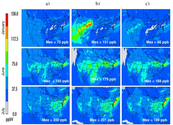
Figures 9 and 10, respectively, show the outputs of the av-erage monthly surface ozone concentrations and the maxi-mum monthly surface ozone concentrations for January (top frames), June (middle frames), and July (bottom frames). The maximum ozone concentrations within the domain are also listed at the corner and denoted in blue or white. In Fig. 9, the output results show that similar ozone concentra-tion patterns are found across the CONUS domain among all three BCs with some exceptional high ozone being observed in the ORDY-BC. It is believed that these high ozone concen-trations occurring in the Western United States in ORDY-BC are the consequence of high ozone observed at the top layer of CMAQ boundaries discussed earlier. The undesirable boundary conditions (i.e., ORDY-BC) produce abnormal
J
anua
ry
J
une
Ju
ly
Max = 55 ppb
Max = 62 ppb
Max = 66 ppb Max = 55 ppb
Max = 62 ppb
Max = 66 ppb
Max = 50 ppb
Max = 64 ppb
Max = 66 ppb Max = 50 ppb
Max = 64 ppb
Max = 66 ppb Max = 69 ppb
Max = 70 ppb
Max = 69 ppb Max = 69 ppb
Max = 70 ppb
Max = 69 ppb
a)
b)
c)
Fig. 9. Comparisons of monthly average ozone concentrations in January, June and July from CMAQ outputs;(a)Profile-BC (left),(b)
ORDY-BC (middle), and(c)Tropo-BC (right). The maximum concentration within the domain is shown at the bottom of right hand corner.
J
a
nuar
y
J
une
Ju
ly
a)
b)
c)
Max = 75 ppb
Max = 165 ppb
Max = 200 ppb Max = 75 ppb
Max = 165 ppb
Max = 200 ppb
Max = 151 ppb
Max = 179 ppb
Max = 201 ppb Max = 151 ppb
Max = 179 ppb
Max = 201 ppb
Max = 66 ppb
Max = 169 ppb
Max = 199 ppb Max = 66 ppb
Max = 169 ppb
Max = 199 ppb
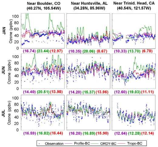
Fig. 11. Comparison of simulated and measured surface ozone concentration for month of January, June and July from the selected sites. The quoted value at the bottom of each plot revives the root mean square error of each case.
observed between ORDY-BC and Profile-BC/Tropo-BC re-veal an important message, which is “excluding stratospheric ozone on tropospheric model during the downscaling pro-cess is extremely important. We have found the concentra-tion differences between these scenarios could be as much as 87 ppbv in January. These differences gradually decrease with temperature increasing through June and July. The ef-fects of lateral BCs in ORDY-BC have contributed to the high surface concentrations observed in the western United States in January and June. Since both ORDY-BC and Tropo-BC utilize a dynamic algorithm to interpolate the vertical ozone profile for each horizontal grid for lateral BCs, the variations in the western boundary are observed primarily due to the treatments of stratospheric ozone. Note that the Tropo-BC is intended to demonstrate the effectiveness of the tropopause-determining algorithm of separating the stratospheric and tropospheric ozone for the lateral boundary condition.
7.3 CMAQ performance analyses
Model performance analyses on all three cases have been performed using the entire CASTNET dataset, in which 70+ observation sites across the CONUS domain from both EPA
and the National Park Service (NPS) are included. It should be noted that our study only simulates the 36 km domain and it is intended to demonstrate the effects of different BCs. Hence, the results in root mean square error in this research may be higher than the one in a finer resolution CMAQ. Fig-ure 11 shows the simulated and measFig-ured surface ozone for the months of January, June, and July at the nearest loca-tions of the ozonesonde sites found in CASTNET network (see Fig. 3 denoted in red star). In the plot, blue, purple, green, and red colors correspond to observation, Profile-BC, ORDY-BC, and Tropo-BC, respectively. And the top, mid-dle, and bottom panels show the first 15 day’s outputs for Jan-uary, June, and July, respectively. It should be noted that, due to limitation of the size of the plot, we have only documented the first 15 days of data in Fig. 11. However, our analyses are based on a full month of data. The quoted number be-low each point represents root mean square error (RMSE) for each case, with the same color scheme used on the plot.
7.3.1 ORDY-BC
a)
b)
NET-RMSE Predicted (ppbv)
0 5 10 15 20 25 30
NE
T
-R
M
S
E
A
c
tual
(
ppbv)
0 5 10 15 20 25 30
January June June<252K July
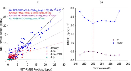
JAN: NET-RMSE=459.7-1.59(Avg_temp) -1.69(LAT), R2=0.73
JUL: RMSE=6.73-0.02(Avg_temp), R2=0.01
JUN<252: NET-RMSE=203.9-0.81(Avg_temp), R2=0.52 JUN: NET-RMSE=108.87-0.42(Avg_temp), R2=0.3
Temperature (K)
248 250 252 254 256 258 260
R
M
SE
(
p
pbv)
/
R
2
0.0 0.5 1.0 1.5 2.0 2.5 3.0
R2
RMSE
Fig. 12. Statistical analysis outputs from CASTNET sites: (a)NET-RMSE actual vs. NET-RMSE predicted,(b)sensitivity analysis on best-fit equation for June data.
June (i.e., top and middle panels) and it is in agreement with our results early in Fig. 10. In comparisons of RMSE, ORDY-BC has shown the worst prediction of surface ozone comparing with others. The RMSE reaches as much as 23.0 ppbv. The highest RMSE occurs at the conditions where the tropopause is low in January and at “near Boulder” site (top left panel). This large RMSE strongly ties to the pa-rameters such as air temperature, altitudinal, and latitudinal locations. Since “near Boulder” is located much higher in al-titude (i.e., Boulder at about 1650 m above mean sea level) than Huntsville and Trinidad head, the larger amount and quicker downshift of uncontrolled stratospheric ozone is ex-pected at the surface of ORDY-BC. This did not happen in Profile-BC and Tropo-BC since both of them do not con-tain any stratospheric ozone. For air temperature, January has much lower air temperature than June and July. With the relationship of air temperature, it is directly proportional to tropopause height; lower air temperature means a lower tropopause height. Therefore, a larger amount of aloft ozone is included in the lateral boundary condition of ORDY-BC and results from a huge over prediction of surface ozone in “near Boulder”. This low temperature effect has also con-tributed to the high RMSE found in “near Huntsville” and “near Trinidad head” sites in January.
Another high RMSE(s) is found in “near Boulder” and “near Trinidad head” in June. These high RMSE(s) most likely relate to the low tropopause height resulting from low air temperature. We believe latitudinal location might ex-plain why “near Boulder” and “near Trinidad head” observed high RMSE, where as “near Huntsville” did not. In gen-eral, the higher latitudinal location is, the lower temperature will be when it is further away from the equator. The low temperature condition affects the downscaling process by
Table 2.Summary of NET-RMSE and average column temperatures for the sonde sites.
Boulder, CO Huntsville, AL Trinidad head, CA January Tc = 236 K Tc = 246 K Tc = 242 K
NET-RMSE = 10.5 ppbv NET-RMSE = 11.4 ppbv NET-RMSE = 6.9 ppbv June Tc = 247 K Tc = 254 K Tc = 252 K
NET-RMSE = 6.5 ppbv NET-RMSE = 1.4 ppbv NET-RMSE = 7.9 ppbv July Tc = 253 K Tc = 257 K Tc = 255 K
NET-RMSE = 0.39 ppbv NET-RMSE = 1.0 ppbv NET-RMSE = 0.1 ppbv
Tc is average vertical column temperature; NET-RMSE is the RMSE differences between Profile-BC and Tropo-BC.
effect, we have performed sensitive fittings on June’s data because it contains both stratospheric effect sites and non-stratospheric effect sites. Figure 12b shows the results of the sensitive test and the observed break point temperature is about 252 K, at which the lowest RMSE and the highest R2are obtained. These results are consistent with our early explanations of why bad predictions of ORDY-BC occurred in January and June and similar predictions as Tropo-BC are found in July. Table 2 shows the monthly average column temperature along with NET-RMSE in all three ozonesonde sites for all months. For January, all three sites have the av-erage temperature lower than 252 K. Therefore, a large NET-RMSE caused from stratospheric ozone is expected. For June, Boulder and Trinidad head are equal or below 252 K, where as Huntsville is above 252 K. Hence, a large RMSE(s) is observed in those two sites and a small NET-RMSE is found in Huntsville. These results are in agreement with our conclusions made earlier on the time-series plots in Fig. 11. Overall, these results stress the important rela-tionship of temperature and seasonal changes in the GCM downscaling process.
7.3.2 Profile-BC
For Profile-BC versus lateral boundary conditions from GCTM, Tang et al. (2007, 2009), have found that the perfor-mance of boundary conditions from GCTM may not neces-sarily be better than Profile-BC. Moreover, different GCTM outputs also yield different results. The performance of lat-eral boundary conditions from GTCM (GCTM-LBC) highly depends on locations and scenarios of the GCTM-LBC, also the type of GCTM used. Al-Saadi et al. (2007), suggested that this phenomenon might relate to the ozone aloft in GCTM-LBC, where rapid transports of stratospheric ozone into the surface level are observed. In addition, they have found that GCTM-LBC enhances the model errors of ozone concentration at the surface in the range of 6 to 20 ppbv in Trinidad Head in August. Since these studies have se-lected the summer ozone season (i.e., August) as their study period, we expected that the effect of stratospheric ozone would be minimal based on the relationship we developed earlier. However, this did not happen. In this case, we
sus-pect their average column temperature in August for Trinidad head may not be hot enough to exclude the stratospheric ozone from the GCTM-LBC interpolating process, or it may be affected by the quality of GCTM-LBC as inputs where strong boundary influx of ozone affects the simulation re-sults. Nevertheless, these studies have indicated that GCTM-LBC preprocessing may be required. In our study, we have implemented the tropopause-determining algorithm, which is based on chemical tropopause definition, as the prepro-cessor for generating ORDY-BC and denoted at Tropo-BC. Note that ORDY-BC is one kind of GCTM-LBC. The inten-tion of the tropopause algorithm is an attempt to improve the ozone simulation at the surface. Figure 11 shows the RMSE for both Profile-BC and Tropo-BC. The results show that the RMSE in Profile-BC is always higher than the RMSE in Tropo-BC, where as the ORDY-BC have either greater or less than Profile BC depending on the locations. Al-though the differences between Profile-BC and Tropo-BC in RMSE was found to be within 1 to 2 ppbv in June and July, and 3 to 4 ppbv in January, the results have demonstrated the tropopause-determining algorithm has successfully pre-vented the high surface ozone estimates, which Tang and Al-Saadi mentioned in their study.
7.3.3 Tropo-BC
Table 3.Summary of NET-RMSE and average column temperatures for the sonde sites.
Profile-BC Tropo-BC ORDY-BC January All RMSE = 11.9 ppbv RMSE = 10.3 ppbv RMSE = 19.8 ppbv
MB = 7.3 ppbv MB = 3.9 ppbv MB = 13.2 ppbv West RMSE = 16.8 ppbv RMSE = 13.0 ppbv RMSE = 23.5 ppbv
MB = 14.6 ppbv MB = 9.8 ppbv MB = 18.3 ppbv Central RMSE = 10.1 ppbv RMSE = 8.2 ppbv RMSE = 23.6 ppbv
MB = 6.6 ppbv MB = 2.4 ppbv MB = 16.1 ppbv East RMSE = 11.2 ppbv RMSE = 10.1 ppbv RMSE = 18.0 ppbv
MB = 6.3 ppbv MB = 3.2 ppbv MB = 11.5 ppbv June All RMSE = 14.3 ppbv RMSE = 13.8 ppbv RMSE = 16.4 ppbv
MB = 0.3 ppbv MB = 1.9 ppbv MB = 7.2 ppbv West RMSE = 18.3 ppbv RMSE = 15.2 ppbv RMSE = 19.9 ppbv
MB = 4.3 ppbv MB = 2.0 ppbv MB = 7.2 ppbv Central RMSE = 12.5 ppbv RMSE = 11.3 ppbv RMSE = 16.0 ppbv
MB =−4.5 ppbv MB =−1.3 ppbv MB = 6.1 ppbv East RMSE = 14.1 ppbv RMSE = 14.1 ppbv RMSE = 15.9 ppbv
MB = 1.1 ppbv MB = 2.9 ppbv MB = 7.6 ppbv July All RMSE = 16.3 ppbv RMSE = 15.8 ppbv RMSE = 16.6 ppbv
MB = 4.2 ppbv MB = 3.4 ppbv MB = 5.3 ppbv West RMSE = 19.8 ppbv RMSE = 16.9 ppbv RMSE = 16.9 ppbv
MB = 4.3 ppbv MB = 4.1 ppbv MB = 6.0 ppbv Central RMSE = 13.7 ppbv RMSE = 13.3 ppbv RMSE = 13.7 ppbv
MB =−2.4 ppbv MB =−3.1 ppbv MB =−1.4 ppbv East RMSE = 16.4 ppbv RMSE = 16.3 ppbv RMSE = 17.3 ppbv
MB = 6.2 ppbv MB = 6.1 ppbv MB = 8.1 ppbv
All – All stations; West – West of 115 W; Central – Between 115 W and 94 W; East – East of 94 W; RMSE is root mean square error; MB is mean bias.
contributed by the sites that are located in the State of Wash-ington. The magnitude of changing RMSE in the State of Washington ranges from 4 to 12 ppbv. The poor performance of BC in RMSE in the “West” has shown that Profile-BC has failed to estimate the impact from intercontinental transport of air pollutants from East Asia across the Pacific Ocean. Moreover, it fails to represent the actual geospatial variations of lateral boundary in the United States.
For the performance of Tropo-BC in all other regions, mi-nor improvement is observed when compared with Profile-BC. Large improvement is found in month of January. Since Profile-BC uses a fixed BC concentration and this fixed BC concentration is usually higher than the actual background ozone in winter, as a result, overestimation of surface ozone in Profile-BC is observed. This demonstrates the importance of using dynamic BCs instead of the static BCs. Figure 13 shows the distributions of RMSE differences among these three scenarios for each of the CASTNET sites. If we con-sider ±1 ppbv as model variability, then we conclude that only 5% or less of the sites in Tropo-BC have poorer perfor-mance compared with Profile-BC. In these 5% of the sites, we have observed the Tropo-BC overestimated the nighttime ozone concentration in June.
In comparison with ORDY-BC, Tropo-BC is outper-formed for every observation site in January. Strong im-provement in Tropo-BC is found in both January and June. In the plot, we have observed 10% or less of the sites in Tropo-BC have poorer performance than in ORDY-BC (i.e., right side panel). We believed that this 10% is contributed by the nature of underestimation of ozone in 36 km resolution. Since the surface ozone in ORDY-BC is always higher than in Tropo-BC, the improvement may not actually be counted. For the overall performance, Tropo-BC has outperformed ORDY-BC in every month for all regions. These results, once again, demonstrate that the removal of stratospheric ozone using our tropopause-determining algorithm strongly improves the performance of surface ozone simulations in CMAQ.
8 Conclusion
- 4 0 4 8 12 16 20 24
- 4 0 4 8 12 16 20 24
5 10 15 20
5 10 20 30
- 2 0 2 4 6 8 10 12
- 4 0 4 8 12 16 20 24
5 10 15
- 2 0 2 4 6 8 10 12
- 2 0 2 4 6 8 10 12
JUN
J
A
N
JU
L
Co
unt
Co
un
t
Co
unt
Profile-BC - Tropo-BC
RMSE (ppbv)
10 20 30 40 5 10 15 20 2 4 6 8
ORDY-BC - Tropo-BC
RMSE (ppbv)
Fig. 13.Summary of the RMSE distributions for the differences among these three scenarios for each CASTNET sites.
structures between GEOS-Chem (i.e., containing both the tropospheric and stratospheric components) and CMAQ (containing only the tropospheric component). It identifies the height of tropopause from GCTM outputs and applies tropopause ozone concentration as the maximum ozone con-centration at the CMAQ lateral boundary condition. As a re-sult, it excludes any stratospheric ozone from being included in the regional air quality model. Since CMAQ is only de-signed for tropospheric application with no top boundary in-put, any stratospheric ozone or stratospheric intrusion should be considered inapplicable in CMAQ. In our results, we have found that the GCTM output (i.e., GEOS-Chem) with the tropopause-determining algorithm (i.e., Tropo-BC) always yields a better result than that with the fixed BCs (i.e., Profile-BC). Moreover, Tropo-BC also yields better results than that with the GCM BCs (i.e., ORDY-BC). For Profile-BC, we have observed the fixed BCs tend to overestimate surface ozone concentration during wintertime and underestimate in summertime. For ORDY-BC, strong over prediction of sur-face ozone is observed as a result of stratospheric ozone from the upper atmosphere. These results are similar to the find-ings in Tang et al., where a large overestimation is observed in CMAQ surface ozone when applying GCTM-BC. Fortu-nately, using our new tropopause algorithm technique (i.e., Tropo-BC) with the global model input (i.e., GEOS-Chem), we have resolved the high surface ozone issue observed in GCTM-BC, while maintaining good vertical ozone predic-tion in the upper air. For further improving the model simu-lations, we recommended that all vertical layers from MM5
(i.e., 34 layers) should be used in CMAQ, instead of 19 layers created from vertical collapsing. This way, it will break down the original CMAQ top layer into 5 separated layers with a thickness of 1.0 to 1.5 km for vertical transport. It is believed that the top CMAQ layer (i.e., 6 km deep) is relatively too thick; it may give a wrong representation of transport of flux in the upper troposphere.
In statistical analysis, we have performed a correlation study on the average tropospheric column temperature and stratospheric effect using the RMSE differences between ORDY-BC and Tropo-BC. The results show that a break point temperature, which separates the temperature region between stratospheric effect and non-stratospheric effect in the chemical downscaling process, is about 252 K. This value can be used as a quick check to see whether or not a partic-ular region or day in the regional model is having a strato-spheric effect from GCTM-BC. Nevertheless, this tempera-ture is based on statistical analysis and may contain certain statistical errors. Therefore, we recommend only using this value as a screening tool.
Appendix A
GEOS-Chem to CMAQ IC/BC species mapping table
CMAQ CB-IV species GEOS-CHEM species
[NO2] [NOx]
[O3] [Ox]-[NOx]
[N2O5] [N2O5]
[HNO3] [HNO3]
[PNA] [HNO4]
[H2O2] [H2O2]
[CO] [CO]
[PAN] [PAN]+[PMN]+[PPN]
[MGLY] [MP]
[ISPD] [MVK]+[MACR]
[NTR] [R4N2]
[FORM] [CH2O]
[ALD2] 1/2[ALD2]+[RCHO]
[PAR] [ALK4]+[C2H6]+[C3H8]+
[ACET]+[MEK]+ 1/2[PRPE]
[OLE] 1/2[PRPE]
[ISOP] 1/5[ISOP]
[SO2] [SO2]
[NH3] [NH3]
[ASO4J] [SO4]
[ANH4J] [NH4]
[ANO3J] [NIT]+[NITs]
[AECJ] [BCPI]+[BCPO]
[AORGPAJ] [OCPI]+[OCPO]
[AORGBJ] [SOA1]+[SOA2]+[SOA3]+
[SOA4]
Acknowledgements. This work was supported by the US Environ-mental Protection Agency under STAR Agreement R830959 and the Intercontinental transport and Climatic effects of Air Pollutants (ICAP) project. It has not formally been reviewed by the EPA. The views presented in this document are solely those of the authors and the EPA does not endorse any products or commercial services mentioned in this publication. We also thank NSF funded National Institute of Computational Sciences for us to use Kraken supercomputer on this study.
Edited by: F. Dentener
References
Al-Saadi, J., Pierce, B., McQueen, J., Natarajan, M., Kuhl, D., Tang, Y. H., Schaack, T. K., and Grell, G.: Global Forecasting System (GFS) Project: Improving National chemistry forecast-ing and assimilation capabilities, Applications of Environmental Remote Sensing to Air Quality and Public Health, Potomac, MD, 8–9 May 2007.
Bertschi, I. T., Jaffe, D. A., Jaegle, L., Price, H. U., and Den-nison, J. B.: 2002 airborne observations of Pacific trans-port of ozone, CO, volatile organic compounds, and aerosols
to the northeast Pacific: Impacts of Asian anthropogenic and Siberian boreal fire emissions, J. Geophys. Res., 109, D23S12, doi:10.1029/2003JD004328, 2004.
Bethan, S., Vaughan, G., and Reid, S. J.: A comparison of ozone and thermal tropopause heights and the impact of tropopause def-inition on quantifying the ozone content of the troposphere, Q. J. Roy. Meteor. Soc., 122, 929–944, 1996.
Byun, D. and Schere, K. L.: Review of the governing equations, computational algorithms, and other components of the models-3 Community Multiscale Air Quality (CMAQ) modeling system, Appl. Mech. Rev., 59, 51–77, 2006.
Byun, D. W., Moon, N. K., Jacob, D., and Park, R.: Regional trans-port study of air pollutants with linked global tropospheric chem-istry and regional air quality models, 2nd ICAP Workshop, Re-search Triangle Park, NC, USA, 2004.
Chin, M., Diehl, T., Ginoux, P., and Malm, W.: Intercontinental transport of pollution and dust aerosols: implications for regional air quality, Atmos. Chem. Phys., 7, 5501–5517, 2007,
http://www.atmos-chem-phys.net/7/5501/2007/.
Collins, W. J., Derwent, R. G., Garnier, B., Johnson, C. E., Sanderson, M. G., and Stevenson, D. S.: Effect of stratosphere-troposphere exchange on the future tropospheric ozone trend, J. Geophys. Res., 108(D12), 8528, doi:10.1029/2002JD002617, 2003.
Eder, B., and Yu, S. C.: A performance evaluation of the 2004 release of Models-3 CMAQ, Atmos. Environ., 40, 4811–4824, 2006.
Fiore, A., Jacob, D. J., Liu, H., Yantosca, R. M., Fairlie, T. D., and Li, Q.: Variability in surface ozone background over the United States: Implications for air quality policy, J. Geophys. Res., 108(D24), 4787, doi:10.1029/2003JD003855, 2003. Fu, J. S., Jang, C. J., Streets, D. G., Li, Z. P., Kwok, R., Park, R.,
and Han, Z. W.: MICS-Asia II: Modeling gaseous pollutants and evaluating an advanced modeling system over East Asia, Atmos. Environ., 42, 3571–3583, 2008.
Fusco, A. C. and Logan, J. A.: Analysis of 1970-1995 trends in tropospheric ozone at Northern Hemisphere midlatitudes with the GEOS-CHEM model, J. Geophys. Res., 108(D15), 4449, doi:10.1029/2002JD002742, 2003.
Heald, C. L., Jacob, D. J., Fiore, A. M., Emmons, L. K., Gille, J. C., Deeter, M. N., Warner, J., Edwards, D. P., Crawford, J. H., Hamlin, A. J., Sachse, G. W., Browell, E. V., Avery, M. A., Vay, S. A., Westberg, D. J., Blake, D. R., Singh, H. B., Sandholm, S. T., Talbot, R. W., and Fuelberg, H. E.: Asian outflow and trans-Pacific transport of carbon monoxide and ozone pollution: An integrated satellite, aircraft, and model perspective, J. Geophys. Res., 108(D24), 4804, doi:10.1029/2003JD003507, 2003. Heald, C. L., Jacob, D. J., Park, R. J., Alexander, B., Fairlie, T.
D., Yantosca, R. M., and Chu, D. A.: Trans-Pacific transport of Asian anthropogenic aerosols and its impact on surface air quality in the United States, J. Geophys. Res., 111, D14310, doi:10.1029/2005JD006847, 2006.
Hoinka, K. P.: The tropopause: discovery, definition, and demarca-tion, Meteorol. Z., 6, 281–303, 1997.
Holton, J. R., Haynes, P. H., McIntyre, M. E., Douglass, A. R., Rood, R. B., and Pfister, L.: Stratosphere-Troposphere Ex-change, Rev. Geophys., 33, 403–439, 1995.
Condi-tions: “Tropopause effect”, The 7th Annual CMAS Conference, Chapel Hill, NC, USA, 2008.
Li, Z., Fu, J. S., Jang, C., Wang, B., Mathur, R., Park, R., and Jacob, D.: Evaluation of GEOS-CHEM/CMAQ Interface Over China and US, The 2nd GEOS–Chem Users’ Meeting, Cam-bridge, MA, USA, April, 2005.
Liang, Q., Jaegle, L., Hudman, R. C., Turquety, S., Jacob, D. J., Av-ery, M. A., Browell, E. V., Sachse, G. W., Blake, D. R., Brune, W., Ren, X., Cohen, R. C., Dibb, J. E., Fried, A., Fuelberg, H., Porter, M., Heikes, B. G., Huey, G., Singh, H. B., and Wennberg, P. O.: Summertime influence of Asian pollution in the free tro-posphere over North America, J. Geophys. Res., 112, D12S11, doi:10.1029/2006JD007919, 2007.
Lin, J. T., Wuebbles, D. J., and Liang, X. Z.: Effects of interconti-nental transport on surface ozone over the United States: Present and future assessment with a global model, Geophys. Res. Lett., 35, L02805, doi:10.1029/2007GL031415, 2008.
Liu, X., Chance, K., Sioris, C. E., Kurosu, T. P., Spurr, R. J. D., Martin, R. V., Fu, T. M., Logan, J. A., Jacob, D. J., Palmer, P. I., Newchurch, M. J., Megretskaia, I. A., and Chatfield, R. B.: First directly retrieved global distribution of tropospheric column ozone from GOME: Comparison with the GEOS-CHEM model, J. Geophys. Res., 111, D02308, doi:10.1029/2005JD006564, , 2006.
Martin, R. V., Jacob, D. J., Logan, J. A., Bey, I., Yantosca, R. M., Staudt, A. C., Li, Q. B., Fiore, A. M., Duncan, B. N., Liu, H. Y., Ginoux, P., and Thouret, V.: Interpretation of TOMS ob-servations of tropical tropospheric ozone with a global model and in situ observations, J. Geophys. Res., 107(D18), 4351, doi:10.1029/2001JD001480, 2002.
Mathur, R., Lin, H. M., McKeen, S., Kang, D., and Wong, D.: Three-dimensional model studies of exchange processes in the troposphere: use of potential vorticity to specify aloft O3in re-gional models, The 7th Annual CMAS Conference, Chapel Hill, NC, USA, 2008.
McPeters, R. D., Labow, G. J., and Logan, J. A.: Ozone climatolog-ical profiles for satellite retrieval algorithms, J. Geophys. Res., 112, D05308, doi:10.1029/2005JD006823, 2007.
Morris, R. E., McNally, D. E., Tesche, T. W., Tonnesen, G., Boy-lan, J. W., and Brewer, P.: Preliminary evaluation of the commu-nity multiscale air, quality model for 2002 over the southeastern United States, J. Air Waste Manage., 55, 1694–1708, 2005. Morris, R. E., Koo, B., Tesche, T. W., Loomis, C., Stella, G.,
Ton-nesen, G., and Wang, Z.: VISTAS Emissions and Air Quality Modeling - Phase I Task 6 Report: Modeling Protocol for the VISTAS Phase II Regional Haze Modeling, Novato, CA, USA, 2006.
Newchurch, M. J., Ayoub, M. A., Oltmans, S., Johnson, B., and Schmidlin, F. J.: Vertical distribution of ozone at four sites in the United States, J. Geophys. Res., 108(D1), 4031, doi:10.1029/2002JD002059, 2003.
Ordonez, C., Brunner, D., Staehelin, J., Hadjinicolaou, P., Pyle, J. A., Jonas, M., Wernli, H., and Prevot, A. S. H.: Strong in-fluence of lowermost stratospheric ozone on lower tropospheric background ozone changes over Europe, Geophys. Res. Lett., 34, L07805, doi:10.1029/2006GL029113, 2007.
Park, R. J., Jacob, D. J., Chin, M., and Martin, R. V.: Sources of carbonaceous aerosols over the United States and implica-tions for natural visibility, J. Geophys. Res., 108(D12), 4355,
doi:10.1029/2002JD003190, 2003.
Park, R. J., Jacob, D. J., Field, B. D., Yantosca, R. M., and Chin, M.: Natural and transboundary pollution influ-ences on sulfate-nitrate-ammonium aerosols in the United States: Implications for policy, J. Geophys. Res., 109, D15204, doi:10.1029/2003JD004473, 2004.
Park, R. J., Jacob, D. J., Kumar, N., and Yantosca, R. M.: Regional visibility statistics in the United States: Natural and transbound-ary pollution influences, and implications for the Regional Haze Rule, Atmos. Environ., 40, 5405–5423, 2006.
Perez, C., Jimenez, P., Jorba, O., Sicard, M., and Baldasano, J. M.: Influence of the PBL scheme on high-resolution photochemical simulations in an urban coastal area over the Western Mediter-ranean, Atmos. Environ., 40, 5274–5297, 2006.
Song, C. K., Byun, D. W., Pierce, R. B., Alsaadi, J. A., Schaack, T. K., and Vukovich, F.: Downscale linkage of global model output for regional chemical transport modeling: Method and general performance, J. Geophys. Res., 113, D08308, doi:10.1029/2007JD008951, 2008.
Stohl, A., Bonasoni, P., Cristofanelli, P., Collins, W., Feichter, J., Frank, A., Forster, C., Gerasopoulos, E., Gaggeler, H., James, P., Kentarchos, T., Kromp-Kolb, H., Kruger, B., Land, C., Meloen, J., Papayannis, A., Priller, A., Seibert, P., Sprenger, M., Roelofs, G. J., Scheel, H. E., Schnabel, C., Siegmund, P., Tobler, L., Trickl, T., Wernli, H., Wirth, V., Zanis, P., and Zerefos, C.: Stratosphere-troposphere exchange: A review, and what we have learned from STACCATO, J. Geophys. Res., 108(D12), 8516, doi:10.1029/2002JD002490, 2003.
Streets, D. G., Fu, J. H. S., Jang, C. J., Hao, J. M., He, K. B., Tang, X. Y., Zhang, Y. H., Wang, Z. F., Li, Z. P., Zhang, Q., Wang, L. T., Wang, B. Y., and Yu, C.: Air quality during the 2008 Beijing Olympic Games, Atmos. Environ., 41, 480–492, 2007.
Tagaris, E., Manomaiphiboon, K., Liao, K. J., Leung, L. R., Woo, J. H., He, S., Amar, P., and Russell, A. G.: Impacts of global climate change and emissions on regional ozone and fine partic-ulate matter concentrations over the United States, J. Geophys. Res., 112, D14312, doi:10.1029/2006JD008262, 2007.
Tang, Y. H., Carmichael, G. R., Thongboonchoo, N., Chai, T. F., Horowitz, L. W., Pierce, R. B., Al-Saadi, J. A., Pfister, G., Vukovich, J. M., Avery, M. A., Sachse, G. W., Ryerson, T. B., Holloway, J. S., Atlas, E. L., Flocke, F. M., Weber, R. J., Huey, L. G., Dibb, J. E., Streets, D. G., and Brune, W. H.: Influ-ence of lateral and top boundary conditions on regional air qual-ity prediction: A multiscale study coupling regional and global chemical transport models, J. Geophys. Res., 112, D10S18, doi:10.1029/2006JD007515, 2007.
Tang, Y. H., Lee, P., Tsidulko, M., Huang, H. C., McQueen, J. T., DiMego, G. J., Emmons, L. K., Pierce, R. B., Thompson, A. M., Lin, H. M., Kang, D., Tong, D., Yu, S. C., Mathur, R., Pleim, J. E., Otte, T. L., Pouliot, G., Young, J. O., Schere, K. L., David-son, P. M., and Stajner, I.: The impact of chemical lateral bound-ary conditions on CMAQ predictions of tropospheric ozone over the continental United States, Environ. Fluid Mech., 9(1), 43–58, doi:10.1007/s10652-008-9092-5, 2008.
Tesche, T. W., Morris, R., Tonnesen, G., McNally, D., Boylan, J., and Brewer, P.: CMAQ/CAMx annual 2002 performance evalua-tion over the eastern US, Atmos. Environ., 40, 4906–4919, 2006. Vingarzan, R.: A review of surface ozone background levels and
WMO, Atmospheric ozone, 1985: WMO Global Ozone Res. and Monit. Proj. Rep. 20, World Meteorological Organization (WMO), Geneva, Switzerland, 1986.