www.geosci-model-dev.net/9/3617/2016/ doi:10.5194/gmd-9-3617-2016
© Author(s) 2016. CC Attribution 3.0 License.
Equilibrium absorptive partitioning theory between multiple
aerosol particle modes
Matthew Crooks, Paul Connolly, David Topping, and Gordon McFiggans
The School of Earth, Atmospheric and Environmental Science, The University of Manchester, Oxford Road, Manchester, M13 9PL, UK
Correspondence to:Matthew Crooks ([email protected])
Received: 18 August 2015 – Published in Geosci. Model Dev. Discuss.: 19 January 2016 Revised: 19 August 2016 – Accepted: 4 September 2016 – Published: 12 October 2016
Abstract. An existing equilibrium absorptive partitioning model for calculating the equilibrium gas and particle con-centrations of multiple semi-volatile organics within a bulk aerosol is extended to allow for multiple involatile aerosol modes of different sizes and chemical compositions. In the bulk aerosol problem, the partitioning coefficient determines the fraction of the total concentration of semi-volatile mate-rial that is in the condensed phase of the aerosol. This work modifies this definition for multiple polydisperse aerosol modes to account for multiple condensed concentrations, one for each semi-volatile on each involatile aerosol mode. The pivotal assumption in this work is that each aerosol mode contains an involatile constituent, thus overcoming the poten-tial problem of smaller particles evaporating completely and then condensing on the larger particles to create a monodis-perse aerosol at equilibrium. A parameterisation is proposed in which the coupled non-linear system of equations is ap-proximated by a simpler set of equations obtained by set-ting the organic mole fraction in the partitioning coefficient to be the same across all modes. By perturbing the condensed masses about this approximate solution a correction term is derived that accounts for many of the removed complexities. This method offers a greatly increased efficiency in calcu-lating the solution without significant loss in accuracy, thus making it suitable for inclusion in large-scale models.
1 Introduction
which acts as a CCN will, in general, produce a greater num-ber of smaller cloud droplets as there are more particles com-peting for the same available water (Twomey, 1959). In con-trast, according to Köhler theory, the larger aerosol particles in a polydisperse system will have a greater affinity to ac-tivate into cloud droplets and their presence can deplete the available water vapour more quickly than smaller ones, due to their quicker growth rates. Consequently, the presence of a larger CCN can suppress the supersaturation, causing fewer smaller particles to activate (Ghan et al., 1998).
The aforementioned effects of aerosol size and number concentration can alter precipitation rates and, as a result, the lifetime of clouds (Stevens and Feingold, 2009; Albrecht, 1989). In addition to a tangible effect of an increase in number of cloud droplets leading to both an increase in re-flected shortwave radiation and absorbed longwave radiation (McCormick and Ludwig, 1967; Chýlek and Coakley Jr., 1974), there is a complicated interdependency between cloud longevity and albedo (Twomey, 1974, 1977). The result is an approximate 0.7 W m−2decrease in mean global radiative forcing, although this is subject to a large degree of uncer-tainty, which is a similar order of magnitude to the mean total radiative forcing from anthropogenic activity (Forster et al., 2007; Lohmann et al., 2000).
Quantifying the size and chemical composition of indi-vidual aerosol particles within a population is complicated due to them being a heterogeneous mix of primary and sec-ondary particles, as well as secsec-ondary aerosol mass. Primary aerosol particles are emitted directly from biogenic and an-thropogenic sources. Although some models exist to simulate purely semi-volatile primary particles (Tsimpidi et al., 2014), in this paper they are assumed to contain at least a small por-tion of non-volatile material. Secondary aerosol particles are formed by nucleation of vapours to form nanometer-sized particles, while secondary aerosol mass is formed by con-densation of gases onto existing particles. The formation of secondary aerosol mass occurs both on the primary and sec-ondary particles and can increase the size of the secsec-ondary particles to climate-relevant sizes. The condensation process that forms secondary aerosol mass is fairly well understood for inorganic gases (Hallquist et al., 2009); however, there is significant uncertainty associated with the formation of sec-ondary organic aerosol (SOA) from volatile organic com-pounds (VOCs). Part of this uncertainty is a result of the poorly quantified process of oxidation of VOCs to produce SOA and other VOCs with reduced volatility (Jimenez and et al., 2009; Yu, 2011).
Over remote continental regions between 5 and 90 % of the total aerosol mass can be made up of organic material (Andreae and Crutzen, 1997; Zhang et al., 2007; Gray et al., 1986) and a significant proportion of this can be from sec-ondary sources. SOA in such large quantities will act to in-crease the size of the particles as well as significantly change their chemical composition. The effect of the increased size, and consequently soluble mass, is found to be the dominant
effect on cloud, increasing the number of cloud droplets and subsequently decreasing the critical supersaturation (Dusek et al., 2006; Topping et al., 2013).
It is estimated that 104–105 organic species have been measured in the atmosphere, but this may only be a small proportion of the total (Goldstein and Galbally, 2007). Of this number fewer than 3000 have actually been identified (Simpson et al., 2012; Borbon et al., 2013). It is, therefore, impractical to try to model each compound individually. In-stead, fewer surrogate species are used to represent many dif-ferent compounds. O’Donnell et al. (2011), for example, use α-pinene as a surrogate for all monoterpenes and xylene to represent multiple aromatic compounds.
Two popular methods have been developed to simulate multiple organic species using equilibrium absorptive parti-tioning theory (Pankow, 1994), a method of calculating the equilibrium condensed concentrations without solving the computationally expensive dynamic condensation and evap-oration processes. The first (Odum et al., 1996) involves an empirically fitted relation derived from two-compound ex-periments which benefits from its simplicity but, as with any empirical relation, has possibly limited applicability outside of the original constraints. In particular, the approach has been found to be unrealistically sensitive to changes in the concentration of the organics (Cappa and Jimenez, 2010). The second (Donahue et al., 2006) uses a volatility basis set, binning large numbers of semi-volatile organic compounds (SVOCs) into a small number of representative species with effective saturation concentrations. This method was later ex-tended to account for partitioning of both water and SVOCs (Barley et al., 2009) by treating the water as an additional volatile substance.
A limitation of equilibrium absorptive partitioning theory (Pankow, 1994) is the assumption of well-mixed particles. Although some experimental results indicate that aerosol particles containing SOA can exist in highly viscous states (Vaden et al., 2011; Cappa and Wilson, 2011), it is still an active area of research, especially in relation to high relative humidities and the effects on cloud droplet formation. Nu-merical models investigating the effect of diffusion within aerosol particles (Zobrist et al., 2011; Smith et al., 2003) in-dicate a transition from a glassy to liquid phase of the parti-cles above about 50 % relative humidity, which is often en-countered in the atmosphere and is of particular relevance in cloud microphysics.
paper is assumed to have at least a small portion of an in-volatile compound which cannot evaporate into the vapour phase. This assumption is crucial in calculating the equilib-rium vapour/condensed phases on multiple modes as without it, a polydisperse equilibrium does not exist. In the purely volatile particle case, the smaller particles evaporate com-pletely, thus allowing the larger particles to take up additional condensed mass to produce a monodisperse aerosol at equi-librium.
In this paper we present a model for equilibrium absorp-tive partitioning of water and SVOCs onto multiple involatile aerosol modes using the volatility basis set method of Don-ahue et al. (2006). All compounds are considered to be at least partially soluble so that the involatile aerosol influences the partitioning of the SVOCs and the particles are assumed to be always well mixed. The concentration of a SVOC in the condensed phase on one mode has the effect of reduc-ing the total concentration available to the other modes and, as a result, the equilibrium vapour/condensed phases of all the organics on all the involatile modes must be solved for simultaneously. By assuming all modes have approximately the same organic mole fraction, a parameterisation for the solution is derived that has a high degree of accuracy while being significantly more efficient than a standard numerical algorithm would be. Condensed concentrations of organics are compared against equilibrium calculated from a dynamic condensation model and are found be comparable.
2 Equilibrium absorptive partitioning theory for size independent bulk aerosol
Before introducing the new multiple mode equilibrium par-titioning theory, we first review existing parpar-titioning theo-ries, beginning with that for a bulk aerosol. The volatility basis set of Donahue et al. (2006) involves binning multi-ple organic species into groups of compounds with similar saturation concentrations,C∗
j. Each volatility bin is then rep-resented by a single representative species with an effective
C∗
j value. A log10 volatility basis set is used withCj∗values from 1×10⁻⁶to 1×10³µg m−3(Cappa and Jimenez, 2010; Donahue et al., 2006). We use the notation,C∗
j, for the sat-uration concentration measured in µg m−3 to distinguish it from the analogous molar quantity (Barley et al., 2009),Cj∗, in units of µmol m−3obtained by dividingC∗
j by the molec-ular weight. The value ofCj∗is proportional to the saturation vapour pressure,pjo(atm), of the organics in thejth volatility bin at temperature,T0, through the equation
Cj∗=p o jγj106
RT0 . (1)
Here γj is the activity coefficient of the organics in the jth bin,R is the universal gas constant (m3atm mol−1K−1) andT0is the temperature (K). The saturation vapour pressure
is dependent on the temperature, T0, which is taken to be 298.15 K. Conversion to aC∗at another temperature,T, can be done using the Clausius–Clapeyron equation,
C∗(T )=C∗(T0)T0 T exp
−1HRvap 1
T − 1 T0
,
where1Hvapis the enthalpy of vaporisation of the organic compounds and is taken to be 150 kJ mol−1 in the current work.
Water and other inorganic semi-volatile compounds can additionally be considered by binning them along with the organics. For simplicity we ignore inorganic semi-volatiles and for the purposes of applying the theory to the particular problem of cloud physics later in the paper we treat water as a separate volatile compound so that its abundance can be varied independently of the organics.
The total concentration of the SVOCs in thejth volatility bin is defined byCj (µmol m−3) and is decomposed into a vapour and a condensed phase,
Cj=Cjv+Cjc, (2)
indicated by the superposedvandc, respectively. The total concentration of all compounds in the condensed phase,CT, is the sum of the concentration of ions of involatile aerosol, Co, the condensed water,Cw, and each organic component in the condensed phase,
CT =Co+Cw+
X
k
Ckc. (3)
The condensed water can be calculated by assuming ide-ality by equating the saturation ratio,S, to the mole fraction of water,
S= C
w
Co+Cw+P
kCkc
. (4)
Equation (4) can be rearranged to makeCwthe subject and then substituted into Eq. (3) and factorised to give
CT = 1 1−S C
o+X
k Ckc
!
. (5)
The analogous expression to Eq. (4) for the organics is Cjv
Cj∗= Cjc
CT
, (6)
where the saturation ratio has been replaced by the ratio of the vapour pressure to the saturation vapour pressure of the jth component using Eq. (1).
EliminatingCjvfrom Eq. (2) using Eq. (6) and rearranging gives the condensed concentration of thejth organic compo-nent in terms of the total concentration
Cjc=Cj 1+ Cj∗
CT
!−1
The partitioning coefficient is defined as
ξj= 1+ Cj∗
CT
!−1
, (8)
so thatCjc=ξjCj. SinceCT depends on theCjc, this prob-lem must be solved iteratively: calculating the Cjc given an initialCT, using these values to update the value ofCT and repeating until Eq. (5) is satisfied within some tolerance.
3 Equilibrium absorptive partitioning theory for a monodisperse aerosol
The theory in the previous section is independent of the size of the aerosol particles. We extend this theory to include size dependence for a monodisperse aerosol. The partitioning of water is influenced by the size of the aerosol particles through the Kelvin factor,
Kw=exp
4M
wσ ρwRT D
,
whereMw,ρw andσ are the molecular weight, density and surface tension of water, and D is the diameter of the wet aerosol particles. The Kelvin factor multiplies the right-hand side of Eq. (4); see, for example, Rogers and Yau (1996),
S= C
wKw
Co+Cw+P
kCkc
. (9)
Consequently, the right-hand side of Eq. (5) becomes
CT = Kw Kw−S C
o+X
k Ckc
!
, (10)
and for notational simplicity we define the prefactor on the right-hand side byη,
η= K w
Kw−S.
The Kelvin factor for the organics,Kj, is defined by Cai (2005) as
Kj=exp
4Mjσ
ρjRT D
, (11)
whereMjandρjare the molecular weight and density of the organics in thejth volatility bin, andσ is the surface tension of the particle with condensed organics and water. This is included in Eq. (6) in an analogous way to the Kelvin factor for water to give
Cjv
C∗j = CjcKj
CT
, (12)
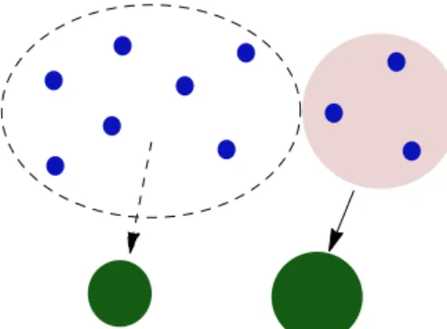
Figure 1.A representation of the condensation of a SVOC, shown by the blue dots, onto two non-volatile particles, shown by the green circles. The SVOC is divided into two groups: those that condense onto the left involatile particle (highlighted in pink) and those re-maining to equilibrate on the right particle (circled by the dashed black line).
and consequently the partitioning coefficient is defined as
ξj= 1+ Cj∗Kj
CT
!−1
. (13)
This set of algebraic equations again needs to be solved iteratively as in the previous section but with the addition of calculating the diameter, and consequently the Kelvin term, from theCjcat each iteration.
4 Equilibrium absorptive partitioning theory for a conglomeration of particles of multiple sizes and composition
An aerosol population commonly comprises particles of dif-ferent sizes and chemical composition. In this section we consider aerosol which can be decomposed into multiple monodisperse aerosol modes. We propose a novel extension to the theory of the previous sections which is applicable to these more diverse conglomerations of particles and there-fore suitable for application to a wider class of problems.
Figure 2.Same as Fig. 1 but with the known number of molecules (highlighted in pink) on the second mode.
available to theith mode is the total concentration in thejth volatility bin minus the condensed concentrations of the or-ganics in thejth bin on the other modes. It is this remaining vapour phase that is multiplied by the partitioning coefficient in the multiple mode case.
We make the following changes to extend the theory in the previous section to the multiple mode case.
– The condensed mass of thejth organic component will now be split across several modes. Define the condensed concentration of thejth organic species on theith in-volatile mode by Cijc so that the condensed phase Cjc can we expressed as the sum
Cjc=X r
Crjc. (14)
For consistency, a subscript i refers to the involatile mode andj refers to thejth volatility bin. Separate in-dicesrandkare used in the summations to make clear which terms are being summed and are applied to sum-mations overiandj, respectively. Subsequently, the to-tal concentration of semi-volatiles in thejth volatility bin is decomposed into a single vapour phase and the sum of the multiple condensed phases
Cj=Cjv+X r
Ccrj. (15)
The total concentration in the condensed phase on the ith mode is given by the sum of the concentrations of the involatile constituent and all of the condensed organics and water on theith mode,
CT ,i=Cio+Ciw+
X
k Cikc,
which can equally be expressed in an analogous way to Eq. (10) as
CT ,i= K w i Kiw−S C
o i +
X
k Cikc
!
. (16)
Here
Kiw=exp
4M
wσ ρwRT Di
is the Kelvin factor of water andCiois the number of µmol per cubic metre of theith involatile aerosol mode. Diis the diameter of theith mode with both condensed water and organics. For notational simplicity we define
ηi = Kiw
Kiw−S, (17)
so that Eq. (16) can be written as
CT ,i=ηi Coi +
X
k Cikc
!
. (18)
– The partitioning coefficient, given by Eq. (13), depends on the material properties and size of the involatile aerosol particles, throughCT andKj, and consequently each volatility bin can have a different coefficient for each mode. The Kelvin factor for thejth volatility bin, Eq. (11), is modified to depend on the diameter of the ith composite mode,Di:
Kij =exp
4M
jσ ρjRT Di
.
Subsequently, the multiple mode analogy to Eq. (12) on theith mode is
Cjv
Cj∗= CijcKij
CT ,i
. (19)
This can be used to eliminate the vapour concentration from Eq. (15):
Cj=
Cj∗CijcKij
CT ,i +
X
r Crjc .
The concentrationCijc can be extracted from the sum on the right-hand side and the equation rearranged to give
Cj−X r6=i
Crjc =Ccij 1+ Cj∗Kij
CT ,i
!
. (20)
We denote the partitioning coefficient for the jth or-ganic component onto theith involatile mode byξij and define it in an analogous way to Eq. (13),
ξij= 1+ Cj∗Kij
CT ,i
!−1
– The total concentration of thejth organic which is avail-able to theith involatile mode, as previously discussed, can now be defined as
Cij=Cj−
X
r6=i Crjc,
or alternatively Cij=Cj−
X
r
Crjc +Cijc. (22)
– An expression for the condensed concentration of the jth organic on theith involatile mode can now be ex-pressed as the product of the partitioning coefficient withCij,
Cijc =
Cj−PrCcrj+Ccij
1+C
∗
jKij CT ,i
, (23)
which is a rearrangement of Eq. (20). Replacing CT ,i using Eq. (18) yields
Cijc =Cj−
P
rCcrj+Ccij
1+ C ∗
jKij/ηi Cio+P
kCikc
. (24)
The non-linear nature of these equations poses a prob-lem for obtaining a solution. Numerical methods exist for solving such problems, but require an initial guess for the solution. Furthermore, there are multiple un-knowns and multi-dimensional non-linear solvers are too computationally expensive to implement in a global climate model. In the following section, we present a method for obtaining an approximate solution to the system of equations represented by Eq. (24), which fa-cilitates a numerical solver in computing the full solu-tion. This approximation, however, is found to be suf-ficiently accurate that an analytic perturbation method, derived in Sect. 5.4, can be used to reduce the inaccura-cies and render the costly numerical solution redundant.
5 A parameterisation for the condensed concentrations We present in this section a proposed parameterisation to cal-culate the condensed concentrations of SVOCs that approx-imate the solution to the multiple mode equilibrium absorp-tive partitioning equations represented by Eq. (24). We begin by simplifying the equations, assuming that all modes share a common average organic mole fraction, and the resulting equations are derived in Sect. 5.2. This approximation can ei-ther be used as an initial condition for a numerical algorithm to solve the full system of equations represented by Eq. (24) or, as we suggest in Sect. 5.4, can be used as a leading-order
solution in a perturbation method in order to derive a correc-tion term that reintroduces many of the removed complexi-ties. We begin by justifying the assumption of the common organic mole fraction.
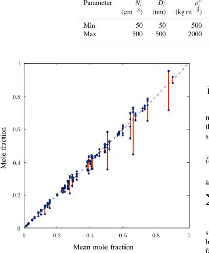
5.1 Motivation
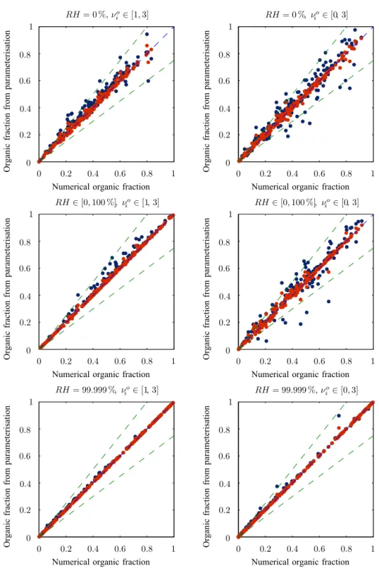
To demonstrate that the individual organic mole fractions of the different modes are comparable, we have run a Monte Carlo simulation that solves the system of equations rep-resented by Eq. (24) for randomly chosen parameter val-ues taken from Table 1. Low accuracy solutions of Eq. (24) for the equilibrium concentrations in the condensed phase are found using a brute force trial and error method. Fifty such solutions for between two and five involatile modes are shown in Fig. 3, with each calculated using different ran-domised parameter values. The concentrations of organics in each volatility bin are kept in the proportions shown in Ta-ble 2 but are rescaled by a random factor of between 0 and 100. Plotted in the graph is the organic mole fraction that we define as the total concentration of semi-volatile material on a mode divided by the total number of ions in the aerosol. For theith mode this is
θi=
P
kCikc Coi +P
kCikc
. (25)
Each solution is represented by several dots joined by a vertical line, with they coordinate of the dots showing the mole fraction of one of the modes. These are plotted against the average mole fraction of all the modes in that solution on thex axis. As can be seen from Fig. 3, even though the mole fractions are different, they never deviate too far from the mean, shown by the dashed line, assuming the same mole fraction for all the modes allows approximate values ofCT ,i to be found in terms of a single parameter. This greatly sim-plifies the problem and can provide a reasonable guess for the non-linear solver.
Table 1.Randomised parameters used to plot Fig. 3.Ni,Di,ρioandMioare the number concentration, diameter, density and molecular
weight of theith involatile aerosol, respectively.νioandνjare the van’t Hoff factors of the involatile constituents and organics.
Parameter Ni Di ρio ρi Mj, Mio νio νj
(cm−3) (nm) (kg m−3) (kg m−3) (kg mol−1)
Min 50 50 500 500 0.1 1 0
Max 500 500 2000 1500 0.4 3 1
Mean mole fraction
M
ol
e
fra
ct
io
n
0 0.2 0.4 0.6 0.8 1
0 0.2 0.4 0.6 0.8 1
Figure 3.The mole fractions of multiple different involatile aerosol modes plotted against the mean mole fraction on thexaxis. Fifty
solutions are shown with parameters randomly chosen from the ranges shown in Table 1 with RH=0 %. The volatility distribution of SVOCs is shown in Table 2, but is rescaled by a random factor of between 0 and 100.
5.2 Derivation of a solution with a common average organic mole fraction
The previous section showed that the organic mole fraction of individual modes is always similar to the mean organic mole fraction across all modes. By making the assumption of a common mole fraction, we now derive a new set of equa-tions to calculate approximate condensed concentraequa-tions of the SVOCs that contain only one unknown in the denomi-nators of the partitioning coefficients. Using a root-finder al-gorithm the common mole fraction can be iterated until it is equal to the mean organic mole fraction across all modes.
The solution derived under the assumption of a common mole fraction,θ, is referred to as the leading-order solution and is denotedCcij. Rearranging Eq. (25) withθi replaced by θgives
θ 1−θ =
P
kC c ik
Cio . (26)
The left-hand side of this equation is the same for all the modes, and consequently the right-hand side must also be the same. For notational simplicity we combine the left-hand side into a single parameter,β,
β= θ 1−θ =
P
kC c ik
Cio , (27)
and subsequently
X
k
Ccik=βCio. (28)
The wet diameter of the combined aerosol is assumed to be sufficiently large that the Kelvin factors for the SVOCs can be approximated by 1. The same is not true for the Kelvin factors for water,Kiw. If these are assumed to take the value 1, then the definition ofηi, as given by Eq. (17), will lead to a gross overestimate of the condensed water close to the cloud base, becoming infinite as the relative humidity be-comes 100 %.
The governing equations for the leading-order solution are obtained by making the approximation given by Eq. (28) to-gether with settingKij =1,
Ccij=Cj−
P
rC c rj+C
c ij
1+ C ∗
j/ηi Cio(1+β)
. (29)
The interdependence of theCcijcan be eliminated to obtain an explicit expression for each in terms of the mole fraction β,
Ccij=C o
i(1+β) 1−φj(β, ηi)
Cj Cj∗/ηi
. (30)
and this will take more time to calculate than the solution to Eq. (30).
The complexity of the summation ofCcijin the denomina-tor has now been removed in favour of a single parameter,β. This can be solved by using a much quicker one-dimensional root find algorithm which iterates the value ofθ, calculating β using Eq. (27) and solving the linear system of equations at each step to find Ccij. The value ofθ can be updated at each iteration based on the average value obtained through Eq. (26), namely,
θ=1 n
X
r
P
kC c rk Cro+P
kC c rk
!
,
wherenis the number of modes. While the dependence ofηionC
c
ij has not been removed, it is sufficiently weak that the values ofCcijcalculated at the previous iteration of θ can be used to evaluate the Kelvin factor for water and thereforeηi, simultaneously converging on the correct value asθis found.
5.3 Results
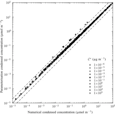
The leading-order solution given in the previous section is calculated and used as an initial guess for a solver of the full non-linear problem; a comparison of the two solutions is pre-sented here. In order to test the theory over a large parameter space, values of the inputs are chosen from Table 1 and the models are run for between two and six modes. Solutions from only one mode are plotted for each run to avoid a bias towards the solutions for six mode runs which would other-wise have 3 times as many points plotted as the two mode runs. Concentrations of the SVOCs are chosen randomly by rescaling the volatility distribution given in Table 2 by be-tween 0 and 100.
Figure 4 shows the individual condensed masses of the 10 volatility bins, each with differently shaped points. The solid black line shows equality between the approximation and the full solution and the dashed lines show 50 % inac-curacies in the approximations. The very strong correlation between the full non-linear solution and the leading-order solution demonstrates that the assumption of a common av-erage organic mole fraction made in the previous section not only offers an efficient way of calculating an initial guess for the non-linear solver, but actually also offers an accurate ap-proximation to the solution for the condensed masses of the organics.
Figure 5 compares the organic mass fractions, defined as the total mass of condensed organics divided by the total mass of the aerosol, from the full non-linear solution and the leading-order solution from the different runs. A range of relative humidities and van’t Hoff factors of the involatile aerosol are used; these values are shown above each plot. Small values of the van’t Hoff factor appear to have a signifi-cant effect on the mass fraction as the correlation of the three
Numerical condensed concentration (µmol m− 3)
Pa
ra
m
et
er
isa
tio
n
co
nd
en
se
d
co
nc
en
tra
tio
n
(µ
m
ol
m
−
3)
C∗(µg m− 3)
10−5 10−4 10−3 10−2 10−1 100 101 102
10−5
10−4
10−3
10−2
10−1
100
101
102
1×10⁻⁶
1×10⁻⁵
1×10⁻⁴
1×10⁻³
1×10⁻²
1×10⁻¹
1×100
1×101
1×10²
1×10³
Figure 4.Comparison of the condensed concentrations of organ-ics from the leading-order solution against those calculated using the non-linear solver for randomly chosen parameters from Table 1. Concentrations of the SVOCs are chosen randomly by rescaling the volatility distribution given in Table 2 by between 0 and 100. The solution is calculated for between two and six modes, and only the condensed concentrations on the first mode are plotted. The differ-ent volatility bins are distinguished by the shape of the points and the correspondingC∗ values given in the legend. The 1:1 line is
shown in solid black and the dashed lines show the 1:2 and 2:1 lines.
right-hand plots is worse than the left three. This is caused by the need to divide by the van’t Hoff factor when converting from number of ions to mass. The result is a high sensitivity of the mass to slight inaccuracies in the number of ions for van’t Hoff factors close to 0; this is addressed in Sect. 5.4.
Table 2.Volatility distribution of SVOCs.
logC∗ −6 −5 −4 −3 −2 −1 0 1 2 3
Cj(µg m−3) 0.005 0.01 0.02 0.03 0.06 0.08 0.16 0.3 0.42 0.8
Numerical organic fraction Numerical organic fraction
Numerical organic fraction Numerical organic fraction
Numerical organic fraction Numerical organic fraction
O
rg
an
ic
fra
ct
io
n
fro
m
pa
ra
m
et
er
isa
tio
n
O
rg
an
ic
fra
ct
io
n
fro
m
pa
ra
m
et
er
isa
tio
n
O
rg
an
ic
fra
ct
io
n
fro
m
pa
ra
m
et
er
isa
tio
n
O
rg
an
ic
fra
ct
io
n
fro
m
pa
ra
m
et
er
isa
tio
n
O
rg
an
ic
fra
ct
io
n
fro
m
pa
ra
m
et
er
isa
tio
n
O
rg
an
ic
fra
ct
io
n
fro
m
pa
ra
m
et
er
isa
tio
n
0 0
0 0
0 0
0.2 0.2
0.2 0.2
0.2 0.2
0.4 0.4
0.4 0.4
0.4 0.4
0.6 0.6
0.6 0.6
0.6 0.6
0.8 0.8
0.8 0.8
0.8 0.8
1 1
1 1
1 1
0 0
0 0
0 0
0.2 0.2
0.2 0.2
0.2 0.2
0.4 0.4
0.4 0.4
0.4 0.4
0.6 0.6
0.6 0.6
0.6 0.6
0.8 0.8
0.8 0.8
0.8 0.8
1 1
1 1
1 1
RH= 0 %, νo
i ∈[1,3] RH= 0 %, ν
o i ∈[0,3]
RH∈[0,100 %],νo
i ∈[1,3] RH∈[0,100 %], ν
o i ∈[0,3]
RH= 99.999 %, νo
i ∈[1,3] RH= 99.999 %,ν
o i ∈[0,3]
5.4 Perturbation solution
Although the condensed masses computed using the approx-imation derived in Sect. 5.2 did not completely agree with the full non-linear solution, the errors were small relative to the size of the Cij. We propose a correction term to this approximation which improves the accuracy and also takes into account the Kelvin terms. Suppose the actual condensed masses,Cijc, can be obtained from the leading-order solution, Ccij, by adding a small perturbation
Cijc =Ccij+ ˆCijc,
where we assume| ˆCijc| ≪ |Ccij|. The Kelvin factors also de-pend on the final condensed mass and for clarity ought to be written asKij=Kij(Cijc). This, however, adds much com-plexity. Therefore, it is assumed that the leading-order solu-tion provides a suitably accurate approximasolu-tion to the con-densed masses of semi-volatiles for the purposes of calcu-lating the Kelvin factors. Consequently, we make the ad-ditional approximation Kij(Cijc)≈Kij(Ccij) which we de-noteKij. Similarly,Kw(Cijc)≈Kw(Ccij)and consequently ηi(Cijc)≈ηi(Ccij)=ηi. We substitute the perturbation into the equations represented by Eq. (24) together with these ap-proximations to give
Ccij+ ˆCcij≈Cj−
P
rC c rj+C
c ij−
P
rCˆrjc + ˆCijc
1+ C
∗
jKij/ηi Cio+P
kC c ik+
P
kCˆikc
. (31)
Assuming the perturbed quantities,Cˆijc, are small, we can
linearise these equations to give 1−ξijˆ
Cijc +ξijX r
ˆ
Crjc −LikX k
ˆ
Cijc
≈Cj− P
rC c rj+C
c ij
1+ C ∗
jKij/ηi Cio+P
kC c ik
−Ccij, (32)
the algebra for which is given in Appendix B. The ξij are the partitioning coefficients, Eq. (21), calculated using the leading-order solution; explicit expressions are given by Eq. (B2). The Lij are defined in Appendix B and are coef-ficients that depend on theCcij as well as the parameters of the problem but are independent of the perturbations. There-fore, these equations are linear in the perturbations and can be solved much quicker than the full set of non-linear equa-tions.
If the leading-order solution, Ccij, were the exact answer, then the right-hand side would simply be a rearrangement of the Eq. (24) and would be zero. In such a situation, the left-hand side would also have to be zero, resulting in a ho-mogeneous system of coupled linear equations with only the
Numerical condensed concentration (µmol m− 3)
Pa
ra
m
et
er
isa
tio
n
co
nd
en
se
d
co
nc
en
tra
tio
n
(µ
m
ol
m
−
3)
C∗(µg m− 3)
10−5 10−4 10−3 10−2 10−1 100 101 102
10−5
10−4
10−3
10−2
10−1
100
101
102
1×10⁻⁶
1×10⁻⁵
1×10⁻⁴
1×10⁻³
1×10⁻²
1×10⁻¹
1×100
1×101
1×10²
1×10³
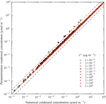
Figure 6.Same as Fig. 4 with the addition of the perturbation solu-tion shown in red.
trivial solution in whichCˆcij=0. However, the leading-order
solution does not satisfy the full system of equations, but is “close” by some measure. Consequently, the right-hand side of Eq. (32) is “small” and defines the size of the small pertur-bationCˆcij. The additional correction term can be calculated
by a simple matrix inversion owing to the linear nature of Eq. (32) which, as we shall see in the following section, pro-duces a much more accurate solution in a fraction of the time it would take to run the non-linear solver.
5.5 Results
Figure 6 is a replica of Fig. 4 with the addition of the con-densed concentrations calculated using the first-order correc-tion term shown in red. The perturbacorrec-tion solucorrec-tion can be seen to offer an improved approximation to the leading-order lution, with almost perfect agreement with the non-linear so-lution for all concentrations.
and improvements in the accuracy of the condensed concen-trations reduce the subsequent errors in the masses.
Figure 8 shows the percentage errors in the calculated mass fractions when compared to the solution from the non-linear solver. The top two plots, which had the worst cor-relation in Fig. 7, show that the leading-order solution pro-duces errors in the organic mass fraction of below 20 % in nearly all cases, and these reduce to 10 % when the correc-tion term in the perturbacorrec-tion solucorrec-tion is included. The affect of van’t Hoff factors close to 0 is most notable in the middle two plots where the errors increase about 3-fold compared to when the van’t Hoff factors are greater than 1: middle right and left plots, respectively. The errors in the perturbation so-lution rarely exceed 10 % across the entire parameter space and are only a few percent at cloud base, shown by the lower two plots.
6 Comparison between the partitioning theory and a dynamic condensation model
The equilibrium absorptive partitioning theory presented in the previous sections calculates the equilibrium condensed concentration of each organic compound. If a dynamic model of condensation of SVOCs is left to run for long enough, it ought to equilibrate on the same solution. We test this in Sect. 6.1 for two modes as a verification of the extension of the partitioning theory to multiple modes. Once we have confirmed that the dynamic model converges on the equi-librium absorptive partitioning theory solution for monodis-perse modes, we investigate the performance of equilib-rium partitioning theory when applied to aerosol modes that are represented by lognormal size distributions in Sect. 6.2, which is more applicable to atmospheric models. Again, a dynamic condensation model is allowed to run until it reaches equilibrium, and this solution is compared to the analogous solution calculated using equilibrium partitioning theory. We have, additionally, simulated two different scenar-ios designed to study how equilibrium absorptive partitioning theory may perform in large-scale models, and the results ap-pear in the Supplement.
6.1 Multiple monodisperse aerosol modes
In this section we confirm that the dynamic model converges on the numerical solution from the equilibrium absorptive partitioning theory for multiple monodisperse modes. This allows us to confirm that the errors encountered in Sect. 6.2 and Sect. S3 of the Supplement are not the result of inac-curacies in the standard equilibrium absorptive partitioning theory presented earlier in the paper.
A dynamic parcel model with binned microphysics by Topping et al. (2013) is modified to maintain constant tem-perature, pressure and water vapour mass; the former two are set to 293.15 K and 95 000 Pa, respectively, and the latter is
calculated from the specified relative humidity. In the simu-lations the time taken for small particles to grow to equilib-rium is of the order of hundreds of seconds, whereas larger particles take thousands. The large particles, however, should take up more of the condensed concentration of the organic compounds due to their higher value of CT. As a conse-quence, the vapour phase equilibrates with the total con-densed concentration very quickly, but the concon-densed mass on smaller particles exceeds equilibrium and consequently deceeds equilibrium on the larger particles. Once the bulk system reaches equilibrium the large particles can only grow at the same rate that the small particles shrink and this pro-cess can take millions of seconds of simulation time to cor-rect to a high degree of accuracy. For the purposes of con-firming convergence of the dynamic model towards the so-lution from equilibrium absorptive partitioning theory it is important to ensure that the dynamic model has converged on an equilibrium to a high degree of accuracy. This solu-tion can then be compared against the equilibrium absorptive partitioning solution to confirm that the two agree.
To obtain accurate convergence of the dynamic model without excessively long simulation times, we start the dy-namic model from a perturbed equilibrium state in which the condensed mass on each mode deceeds equilibrium by a small amount. The dynamic model is initiated with the re-maining organic mass in the vapour phase. Details of how we calculate the initial condensed masses are given in the Sup-plement.
Numerical organic fraction Numerical organic fraction
Numerical organic fraction Numerical organic fraction
Numerical organic fraction Numerical organic fraction
O
rg
an
ic
fra
ct
io
n
fro
m
pa
ra
m
et
er
isa
tio
n
O
rg
an
ic
fra
ct
io
n
fro
m
pa
ra
m
et
er
isa
tio
n
O
rg
an
ic
fra
ct
io
n
fro
m
pa
ra
m
et
er
isa
tio
n
O
rg
an
ic
fra
ct
io
n
fro
m
pa
ra
m
et
er
isa
tio
n
O
rg
an
ic
fra
ct
io
n
fro
m
pa
ra
m
et
er
isa
tio
n
O
rg
an
ic
fra
ct
io
n
fro
m
pa
ra
m
et
er
isa
tio
n
0 0
0 0
0 0
0.2 0.2
0.2 0.2
0.2 0.2
0.4 0.4
0.4 0.4
0.4 0.4
0.6 0.6
0.6 0.6
0.6 0.6
0.8 0.8
0.8 0.8
0.8 0.8
1 1
1 1
1 1
0 0
0 0
0 0
0.2 0.2
0.2 0.2
0.2 0.2
0.4 0.4
0.4 0.4
0.4 0.4
0.6 0.6
0.6 0.6
0.6 0.6
0.8 0.8
0.8 0.8
0.8 0.8
1 1
1 1
1 1
RH= 0 %,νo
i ∈[1,3] RH= 0 %, ν
o i ∈[0,3]
RH∈[0,100 %], νo
i ∈[1,3] RH∈[0,100 %], ν
o i ∈[0,3]
RH= 99.999 %, νo
i ∈[1,3] RH= 99.999 %,ν
o i ∈[0,3]
Figure 7.Same as Fig. 5 with the addition of the perturbation solution shown in red.
Table 3. Material parameters used in the dynamic model simulations. Total SVOC concentrations are 0.47 µg m−3, which represents a rescaling of the volatility distribution given in Table 2 by a factor of 0.25.
Parameter ρio ρj Mj ) Mio νio νj
(kg m−3) (kg m−3) (kg mol−1) (kg mol−1)
0
0
0 0
0 0
10
10 10
20
20
20 20
20 20
30
30 30
40
40
40 40
40 40
50 60
60 60
80 80 100
LO
LO
LO LO
LO LO Perturbation
Perturbation
Perturbation Perturbation
Perturbation Perturbation
RH= 0 %,νo
i∈[1,3] RH= 0 %,ν o i∈[0,3]
RH∈[0,100 %],νo
i∈[1,3] RH∈[0,100 %],νo i∈[0,3]
RH= 99.999 %,νo
i∈[1,3] RH= 99.999 %,ν o i∈[0,3]
Per
cen
ta
ge
er
ro
r
Per
cen
ta
ge
er
ro
r
Per
cen
ta
ge
er
ro
r
Per
cen
ta
ge
er
ro
r
Per
cen
ta
ge
er
ro
r
Per
cen
ta
ge
er
ro
r
Figure 8.Comparison of the percentage errors in organic mass fraction from the two approximations in relation to those calculated using the non-linear solver for the data points in Fig. 7. The leading-order (LO) and perturbation solutions are shown by the left and right box and whisker plots in each figure, respectively.
of the red sections of the bars which, when measured from the x axis, are shown by the horizontal black dashed lines across each bar. These too agree exceptionally well with the pink dashed lines, which are the equivalent values from the partitioning theory.
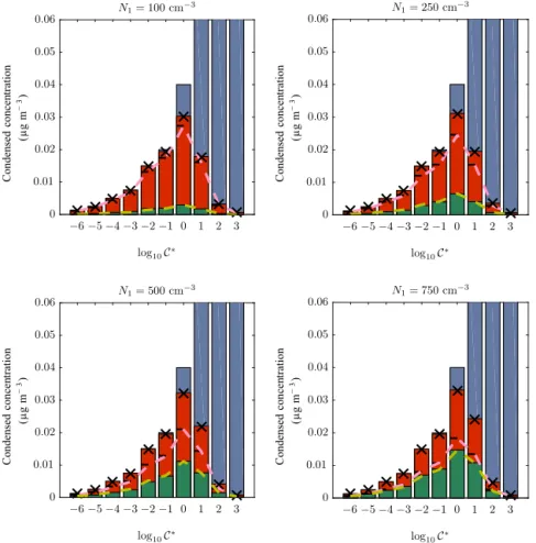
Similar plots are shown in Fig. 10, but this time the size of the first mode is fixed at 50 nm and the number concen-tration is varied instead; the values used are shown above
log10C∗
log10C∗
log10C∗
log10C∗
Co
nd
en
se
d
co
nc
en
tra
tio
n
Co
nd
en
se
d
co
nc
en
tra
tio
n
co
nd
en
se
d
Co
nc
en
tra
tio
n
Co
nd
en
se
d
co
nc
en
tra
tio
n
(µ
g
m
−
3)
(µ
g
m
−
3)
(µ
g
m
−
3)
(µ
g
m
−
3)
−6 −6
−6 −6
−5 −5
−5 −5
−4 −4
−4 −4
−3 −3
−3 −3
−2 −2
−2 −2
−1 −1
−1 −1
0 0
0 0
1 1
1 1
2 2
2 2
3 3
3 3
0 0
0 0
0.01 0.01
0.01 0.01
0.02 0.02
0.02 0.02
0.03 0.03
0.03 0.03
0.04 0.04
0.04 0.04
0.05 0.05
0.05 0.05
0.06 0.06
0.06
0.06 D
1= 25 nm D1= 50 nm
D1= 75 nm D1= 100 nm
3]
Figure 9.Stacked bar charts showing the condensed concentrations from the two models. Each bar shows the total concentration of organics in each volatility bin and is coloured to show the proportion which is in the vapour phase (blue) and the condensed phases on the first and second modes (green and red, respectively). The height of the horizontal black dashed lines across each bar marks the condensed concentrations on the second mode only (the height of the red regions as measured from thexaxis). Total concentrations in each volatility
bin from the partitioning theory are shown by the black crosses and the amounts on the first and second modes are shown by the yellow and pink dashed lines, respectively. Theyaxis is cut off at 0.04 and 0.05 for clarity. The diameter of the first mode is denoted above each plot and
the number concentration is 1000 cm−3, while the second mode has a median diameter of 125 nm and a number concentration of 50 cm−3.
Table 4.Range of values assigned to the number concentration,Ni,
and involatile particle diameter,Di, used in the dynamic model
sim-ulations.
Parameter Ni (cm−3) Di(nm)
Mode 1 100–1000 25–100
Mode 2 50 125
almost equal amounts placed on each of the two modes when the first mode has a number concentration of 750 cm−3. 6.2 Application to lognormally distributed
particle sizes
Aerosol in the atmosphere is often characterised by multiple polydisperse modes with particles in each mode composed of the same chemical composition. The sizes of particles in each mode are described by size distributions which are a
conve-nient way of treating a polydisperse aerosol as each size dis-tribution can be considered as a single entity.
A common assumption is that the diameters of the parti-cles,D, are lognormally distributed so that the number of aerosol particles,N, per logarithmic size interval is given by
dN d lnD =
N
√
2πlnσexp
−
lnD Dm
√
2 lnσ
2
. (33)
HereN is the total number of particles andDmand lnσ are the median diameter and geometric standard deviation. Multiple lognormal size distributions can be added together to form more diverse aerosols:
dN d lnD =
X
i Ni
√
2πlnσiexp
−
ln D Dm,i
√
2 lnσi
2
log10C∗
log10C∗
log10C∗
log10C∗
Co
nd
en
se
d
co
nc
en
tra
tio
n
Co
nd
en
se
d
co
nc
en
tra
tio
n
Co
nd
en
se
d
co
nc
en
tra
tio
n
Co
nd
en
se
d
co
nc
en
tra
tio
n
(µ
g
m
−
3)
(µ
g
m
−
3)
(µ
g
m
−
3)
(µ
g
m
−
3)
−6 −6
−6 −6
−5 −5
−5 −5
−4 −4
−4 −4
−3 −3
−3 −3
−2 −2
−2 −2
−1 −1
−1 −1
0 0
0 0
1 1
1 1
2 2
2 2
3 3
3 3
0 0
0 0
0.01 0.01
0.01 0.01
0.02 0.02
0.02 0.02
0.03 0.03
0.03 0.03
0.04 0.04
0.04 0.04
0.05 0.05
0.05 0.05
0.06 0.06
0.06
0.06 N
1= 100 cm−3 N1= 250 cm−3
N1= 500 cm− 3
N1= 750 cm−3
Figure 10.Same as Fig. 9 but with a differing number concentration of the first mode in each plot and a diameter of 50 nm. The second mode has a median diameter of 125 nm and a number concentration of 50 cm−3.
whereDm,iand lnσi are the median diameter and geometric standard deviation of theith mode.
The difficulty with applying equilibrium partitioning the-ory to size distributions is that particles of different sizes have different Kelvin factors and the semi-volatile organic com-pounds will consequently partition non-uniformly across the sizes of particles. We replace the Kelvin factors by effec-tive values calculated using the median diameters of each mode including the additional condensed mass of SVOCs. For the equilibrium comparisons used in this section, we as-sume that the non-volatile compound is represented by log-normal size distributions of particles. After adding the ad-ditional condensed mass of SVOCs calculated using equi-librium absorptive partitioning, we assume that the particle sizes are also represented by lognormal size distributions. We use the same geometric standard deviation, lnσi, as the non-volatile aerosol modes and assume that the median diameter of each mode increases in order to account for the additional aerosol mass from the SVOCs. In Sect. S4 of the Supplement, we investigate whether, in practice, the geometric standard deviation can be assumed to remain constant while undergo-ing condensation of SVOCs.
Table 5.Parameter values used in the first set of dynamic model simulations.
Parameter N(cm−3) Dm(nm) lnσ
Mode 1 200 25 0.5
Mode 2 50 125 0.1
We begin by comparing the limiting behaviour of the dy-namic model against the equilibrium absorptive partitioning theory, presented in this paper, when each mode is repre-sented by a lognormal size distribution. In order to isolate the errors resulting from the lognormal size distribution ap-proximation in the equilibrium absorptive partitioning theory from errors in the convergence of the dynamic model, we again start the simulations from a perturbed equilibrium con-densed mass. Details of how we derive this initial concon-densed mass are given in Sect. S2 of the Supplement. Further inves-tigations into the applicability of the assumption of equilib-rium in more realistic scenarios and timescales appear in the Supplement.
the-log10C∗ log10C∗
log10C∗ log10C∗
Co
nd
en
se
d
co
nc
en
tra
tio
n
Co
nd
en
se
d
co
nc
en
tra
tio
n
Co
nd
en
se
d
co
nc
en
tra
tio
n
Co
nd
en
se
d
co
nc
en
tra
tio
n
(µ
g
m
−
3)
(µ
g
m
−
3)
(µ
g
m
−
3)
(µ
g
m
−
3)
−6
−6
−6 −6
−5
−5
−5 −5
−4
−4
−4 −4
−3
−3
−3 −3
−2
−2
−2 −2
−1
−1
−1 −1
0 0
0 0
1 1
1 1
2 2
2 2
3 3
3 3
0 0
0 0
0.01
0.01
0.01 0.01
0.02
0.02
0.02
0.02
0.03 0.03
0.03
0.03
0.04 0.04
0.04
0.04
0.05 0.05
0.05 0.05
RH= 0 % RH= 10 %
RH= 50 % RH= 90 %
Figure 11.Same as Fig. 9 for involatile aerosol modes represented by lognormal size distributions with number concentrations of 200 and 50 cm−3and median diameters of 25 and 125 nm, respectively. The geometric standard deviations are 0.5 and 0.1. The relative humidity used in each simulation is stated above each plot.
0.06 0.06
log10C∗ log10C∗
Co
nd
en
se
d
co
nc
en
tra
tio
n
Co
nd
en
se
d
co
nc
en
tra
tio
n
(µ
g
m
−
3)
(µ
g
m
−
3)
−6
−6−5−4−3−2−1 0 1 2 3 −5−4−3−2−1 0 1 2 3
0 0
0.01 0.01
0.02 0.02
0.03 0.03
0.04 0.04
0.05 0.05
RH= 0 % RH= 90 %
Figure 12.Same as Fig. 11, but the first mode has a median diameter of 50 nm and a number concentration of 200 cm−3. The second mode has a median diameter of 125 nm and a number concentration of 50 cm−3. The geometric standard deviations are 0.5 and 0.1.
ory in Fig. 11 for a range of relative humidities. Lognormal size distributions are defined by the parameters in Table 5 with the material properties in Table 3. Total condensed con-centrations from the partitioning theory are shown by the crosses, which lie almost exactly at the top of the red sec-tions which mark the analogous quantity from the dynamic
total condensed concentration as the dynamic model. The condensed concentration on the larger mode is overpredicted by the equilibrium absorptive partitioning theory and conse-quently the condensed mass on the smaller mode is under-predicted by the same amount. Due to the condensed masses on the smaller mode being an order of magnitude less than the larger mode, this error results in a much larger relative error of between 35 and 50 % on the smaller mode. The ef-fect of the increased relative humidity is to increase the total condensed concentration of organics; all of the SVOCs in the five lowest volatility bins are in the condensed phase even at RH=0 %, and so this extra organic mass must come from the higher volatility bins. This is seen by the larger red and green regions for the higher volatility bins in the lower right plot.
The proposed reason for the discrepancies in the con-densed masses on the smaller mode is the effect of the Kelvin factor. The Kelvin factor is most variable for smaller diam-eters, and so using an effective value for all particles within a lognormal mode with a small median diameter results in appreciable errors. To demonstrate this theory, we have car-ried out further simulations with a smaller mode with a me-dian diameter of 50 nm. These are shown in Fig. 12 for rel-ative humidities of 0 and 90 %. As can be seen, the errors in condensed mass on the smaller mode are eradicated and the two equilibrium solutions are in perfect agreement. We con-clude, therefore, that equilibrium partitioning can very accu-rately calculate the equilibrium condensed mass on lognor-mal modes if the median diameter is above about 50 nm. In some situations it may be deemed sufficiently accurate to use equilibrium partitioning with lognormal size distributions at smaller diameters, especially when off-set against the reduc-tion in computareduc-tional complexity compared to solving the dynamic condensation process.
7 Conclusions
This paper presents both a model and an efficient and ac-curate parameterisation of the solution that are suitable for investigations in a wide range of research areas that use equi-librium absorptive partitioning theory. Of particular interest to the authors are cloud droplet activation parameterisations and, ultimately, inclusion in global climate models.
The model itself predicts the equilibrium condensed con-centrations of organics onto multiple monodisperse aerosol modes incredibly accurately compared to the equilibrium so-lution from a dynamic model. This holds true for a range of particle sizes, number concentrations and relative humidities. The proposed parameterisation is found to be exception-ally accurate for a wide range of parameters. Assuming the same mole fraction for all of the modes offers a quick method of obtaining a reasonably accurate approximation for all but the smallest van’t Hoff factors of the involatile compounds, but performs well at high values of relative humidity. The perturbation correction term offers significant improvements at lower relative humidity, especially for smaller van’t Hoff factors, with a negligible increase in computational expense. The condensed mass calculated using equilibrium absorp-tive partitioning theory with lognormal size distributions of involatile particles agrees very well with the limiting be-haviour of the dynamic model if the median diameters of the modes are above 50 nm. Below this size the Kelvin term be-comes important and results in non-negligible errors. This is further corroborated in the more realistic scenarios simulated in the Supplement.
8 Code availability
Appendix A
The implicit equations governing the leading-order solution can be manipulated to give an explicit expression for each of the condensed concentrations, Cij, in terms of the average mole fraction. We present the algebra for such a step here. The coupled equations are given by Eq. (29) and are restated here:
Ccij=Cj−
P
rC c rj+C
c ij
1+ Cj∗/ηi Cio(1+β)
.
We can make use of the notation given by Eq. (14) to write the summation term asCcj and rearrange the denominator on the right-hand side to give
Ccij=Cj−C c j+C
c ij
Co
i(1+β) Cio(1+β)+Cj∗/ηi
.
The explicit dependence onCcij can be factorised onto the left-hand side:
Cj∗/ηi
Cio(1+β)+Cj∗/ηi
!
Ccij=
Coi(1+β)Cj−Ccj
Cio(1+β)+Cj∗/ηi ,
which further reduces to
Ccij=
Cio(1+β)Cj−Ccj
Cj∗/ηi
. (A1)
By summing overian equation forCcjis obtained,
Ccj=Cj−C c j
X
r
Cro(1+β) Cj∗/ηr
,
which has the solution Ccj=φjCj,
whereφj depends onβ andηiand is given by
φj(β, ηi)=
P
r
Cro(1+β) Cj∗/ηr
1+P
r
Cor(1+β) Cj∗/ηr
, (A2)
The individual condensed concentrations are then calcu-lated using Eq. (A1), which can now be written as
Ccij=C o
i(1+β) 1−φjCj Cj∗/ηi
.
Appendix B
The details of the linearisation of the perturbation Eq. (31) are presented in this appendix and we begin by restating the set of non-linear equations
Ccij+ ˆCijc =Cj−
P
rC c rj+C
c ij−
P
rCˆrjc + ˆCijc
1+ C
∗
jKij/ηi Cio+P
kC c ik+
P
kCˆikc .
The denominator on the right-hand side can be rearranged to give
Ccij+ ˆCijc = Cj−
X
r
Ccrj+Ccij−X r
ˆ
Crjc + ˆCijc
! × C o i + P kC c ik+ P
kCˆikc Cio+P
kC c ik+
P
kCˆikc +Cj∗Kij/ηi
!
= Cj−
P
rC c rj+C
c ij−
P
rCˆrjc + ˆCijc Cio+P
kC c
ik+C∗jKij/ηi
! ×
Cio+P
kC c ik+
P
kCˆikc
1+
P
kCˆikc Cio+P
kC c
ik+Cj∗Kij/ηi
= Cj−
P
rC c rj+C
c ij−
P
rCˆrjc + ˆCijc Cio+P
kC c
ik+C∗jKij/ηi
!
× Cio+X k
Ccik+X k
ˆ
Cikc
!
× 1+
P
kCˆikc Cio+P
kC c
ik+Cj∗Kij/ηi
!−1
.
We now assume that the perturbations are sufficiently small that P
kCˆikc Cio+P
kC c
ik+Cj∗Kij/ηi
≪1, (B1)
so that the third term on the right-hand side can be approxi-mated by its Taylor series expansion of the form
1
withxequal to the term (B1),
Ccij+ ˆCcij=
Cj−PrC c rj+C
c ij−
P
rCˆrjc + ˆCijc Coi +P
kC c
ik+Cj∗Kij/ηi
!
× Cio+X k
Ccik+X k
ˆ
Cikc
!
× 1−
P
kCˆikc Cio+P
kC c
ik+C∗jKij/ηi
+O
h
ˆ
Cijci2
!
.
The right-hand side can be linearised assuming the terms of orderO
h
ˆ
Cijci2
are negligible.
Ccij+ ˆCcij≈Cj−
P
rC c rj+C
c ij
1+ C ∗
jKij/ηi Cio+P
kC c ik
+ −
P
rCˆrjc + ˆCijc
1+ C ∗
jKij/ηi Coi +P
kC c ik
+ Cj−
P
rC c rj+C
c ij
Coi +P
kC c
ik+Cj∗Kij/ηi
! X
k
ˆ
Cikc
−
Cj−PrC c rj+C
c
ij Cio+
P
kC c ik
Cio+P
kC c ik+
Cj∗Kij
ηi
!2
X
k
ˆ
Cikc
We can factorise this to give
ˆ
Cijc +
P
rCˆrjc − ˆCijc
1+ C ∗
jKij/ηi Cio+P
kC c ik
−
Cj−PrC c rj+C
c ij
Cj∗Kij
ηi
Cio+P kC
c ik+
Cj∗Kij
ηi
!2
X
k ˆ
Cikc
≈Cj− P
rC c rj+C
c ij
1+ C ∗
jKij/ηi Coi +P
kC c ik
−Ccij.
By denoting the coefficient in the square brackets byLij together with
ξij= 1+ C
∗
jKij/ηi Cio+P
kC c ik
!−1
, (B2)
this expression can be made more notationally simplistic: 1−ξij ˆ
Cijc +ξijX r
ˆ
Crjc −LikX k
ˆ
Cijc
≈Cj− P
rC c rj+C
c ij
1+ C ∗
jKij/ηi Cio+P
kC c ik
−Ccij.
It is important to note that both ξij and Lij depend on the leading-order solution but are independent of the pertur-bation,Cˆijc, and as such this equation is now linear in these