Overview of a prescribed burning experiment within a boreal forest in Finland

(1)

ACPD

13, 21703–21763, 2013

Overview of a prescribed burning

experiment

A. Virkkula et al.

Title Page

Abstract Introduction

Conclusions References

Tables Figures

◭ ◮

Back Close

Full Screen / Esc

Printer-friendly Version Interactive Discussion

Discussion

P

a

per

|

D

iscussion

P

a

per

|

Discussion

P

a

per

|

Discuss

ion

P

a

per

Atmos. Chem. Phys. Discuss., 13, 21703–21763, 2013 www.atmos-chem-phys-discuss.net/13/21703/2013/ doi:10.5194/acpd-13-21703-2013

Atmospheric Chemistry and Physics

Open Access

Discussions

Geoscientiic Geoscientiic

This discussion paper is/has been under review for the journal Atmospheric Chemistry and Physics (ACP). Please refer to the corresponding final paper in ACP if available.

Overview of a prescribed burning

experiment within a boreal forest in

Finland

A. Virkkula1,2, J. Levula1,3, T. Pohja3, P. P. Aalto1, P. Keronen1,

S. Schobesberger1, C. B. Clements4, L. Pirjola5, A.-J. Kieloaho1, L. Kulmala6, H. Aaltonen7, J. Patokoski1, J. Pumpanen7, J. Rinne1, T. Ruuskanen1,

M. Pihlatie1, H. E. Manninen1, V. Aaltonen2, H. Junninen1, T. Petäjä1, J. Backman1, M. Dal Maso1, T. Nieminen1, T. Olsson2, T. Grönholm8,

V.-M. Kerminen1, D. M. Schultz1,2,9, J. Kukkonen2, M. Sofiev2, G. de Leeuw1,2, J. Bäck7, P. Hari7, and M. Kulmala1

1

Department of Physics, University of Helsinki, 00014, Helsinki, Finland

2

Finnish Meteorological Institute, Erik Palménin aukio 1, 00101, Helsinki, Finland

3

Hyytiälä Forestry Field Station, University of Helsinki, 35500, Korkeakoski, Finland

4

Department of Meteorology and Climate Science, San José State University, 95192, San José CA, USA

5

Department of Technology, Metropolia University of Applied Sciences, 00079, Helsinki, Finland

6

(2)

ACPD

13, 21703–21763, 2013

experiment

A. Virkkula et al.

Title Page

Tables Figures

◭ ◮

Back Close

Full Screen / Esc

Discussion

P

a

per

|

D

iscussion

P

a

per

|

Discussion

P

a

per

|

Discuss

ion

P

a

per

|

7

Department of Forest Sciences, P.O. Box 27, 00014, University of Helsinki, Helsinki, Finland

8

Finnish Environment Institute, Joensuu Office, 80101 Joensuu, Finland

9

Centre for Atmospheric Science, School of Earth, Atmospheric and Environmental Sciences, University of Manchester, Simon Building, Oxford Road, Manchester, M13 9PL, UK

Received: 20 June 2013 – Accepted: 29 July 2013 – Published: 22 August 2013

Correspondence to: A. Virkkula (aki.virkkula@helsinki.fi)

(3)

ACPD

13, 21703–21763, 2013

experiment

A. Virkkula et al.

Title Page

Tables Figures

◭ ◮

Back Close

Full Screen / Esc

Discussion

P

a

per

|

D

iscussion

P

a

per

|

Discussion

P

a

per

|

Discuss

ion

P

a

per

Abstract

A prescribed burning of a boreal forest was conducted on 26 June 2009 in Hyytiälä, Finland, to study aerosol and trace gas emissions from wildfires and the effects of fire on soil properties in a controlled environment. A 0.8 ha forest near the SMEAR II was cut clear; some tree trunks, all tree tops and branches were left on the ground and

5

burned. The amount of burned organic material was ∼46.8 t (i.e., ∼60 t ha−1). The flaming phase lasted 2 h 15 min, the smoldering phase 3 h. Measurements were con-ducted on the ground with both fixed and mobile instrumentation, and from a research aircraft. In the middle of the burning area, CO₂concentration peaks were around 2000– 3000 ppm above the baseline and peak vertical flow velocities were 6±3 m s−1, as

10

measured a 10-Hz 3-D sonic anemometer placed within the burn area. Peak particle number concentrations were approximately 1–2×106cm−3in the plume at a distance of 100–200 m from the burn area. The geometric mean diameter of the mode with the highest concentration was at 80±1 nm during the flaming phase and in the middle of the smoldering phase but at the end of the smoldering phase the largest mode was

15

at 122 nm. In the volume size distributions geometric mean diameter of the largest volume mode was at 153 nm during the flaming phase and at 300 nm during the smol-dering phase. The lowest single-scattering albedo of the ground-level measurents was 0.7 in the flaming-phase plume and∼0.9 in the smoldering phase. The radiative forc-ing e_fficiency was negative above dark surfaces, in other words, the particles cool the

20

atmosphere. Elevated concentrations of several VOCs (including acetonitrile which is a biomass burning marker) were observed in the smoke plume at ground level. The forest floor (i.e., richly organic layer of soil and debris, characteristic of forested land) measurements showed that VOC fluxes were generally low and consisted mainly of monoterpenes, but a clear peak of VOC flux was observed after the burning. After

25

(4)

ACPD

13, 21703–21763, 2013

experiment

A. Virkkula et al.

Title Page

Tables Figures

◭ ◮

Back Close

Full Screen / Esc

Discussion

P

a

per

|

D

iscussion

P

a

per

|

Discussion

P

a

per

|

Discuss

ion

P

a

per

|

the available nitrogen contents of the soil, which in turn, affected the level of the long-term fluxes of greenhouse gases.

1 Introduction

Gaseous and aerosol emissions from wildfires have significant climatic and health ef-fects ranging from local to hemispheric scales (e.g., Andreae, 1991; Penner et al., 1992;

5

Grell et al., 2011). In the Northern Hemisphere, smoke from wildfires can be trans-ported over long distances from the boreal forest areas in Eurasia and North America to the Arctic (e.g., Radke et al., 1991; Goldammer et al., 1996; Lavoué et al., 2000; Randerson et al., 2006; Law and Stohl, 2007; Shindell et al., 2008; Paris et al., 2009; Lamarque et al., 2010; AMAP, 2011). Smoke originated from wildland fires in Eastern

10

Europe has also been shown to a_ffect extensive regions in Western and Central Eu-rope (Klein et al., 2012; Saarnio et al., 2010). Wildfire emissions have both warming and cooling effects on climate. The greenhouse gases and black carbon emitted in burning heat the atmosphere but aerosols may also have a cooling e_ffect, depending on their optical and cloud-forming properties. Surface albedo changes due to fires have

15

also a significant climatic effect. For instance, Randerson et al. (2006) showed that the warming impact of increasing boreal forest fires may be limited or even result in re-gional cooling because of loss of canopy overstory and consequently higher albedo values during winter and spring.

Ongoing wildfires and burned areas can be observed from space by using satellite

20

imagery (e.g., Flannigan and Haar, 1986; Lentile et al., 2006; French et al., 2008; Sofiev et al., 2009; van der Werf et al., 2010). Satellite images give information on the area and amount that is burning and also on the amount of smoke released. However, they do not give direct information on the composition of smoke. To estimate the amount of aerosols and trace gases emitted, emission factors, defined as the amount of emitted

25

(5)

ACPD

13, 21703–21763, 2013

experiment

A. Virkkula et al.

Title Page

Tables Figures

◭ ◮

Back Close

Full Screen / Esc

Discussion

P

a

per

|

D

iscussion

P

a

per

|

Discussion

P

a

per

|

Discuss

ion

P

a

per

et al. (2010), Akagi et al. (2011), Simpson et al. (2011), and Yokelson et al. (2013). van der Werf et al. (2010) estimated the total global carbon emissions due to deforesta-tion, savanna, forest, agricultural, and peat fires by using a biogeochemical model and satellite-derived estimates. They estimated that the boreal region accounted for about 9 % of total global carbon emissions from fires.

5

Detailed measurements of gas and aerosol emissions are difficult in real wildfires: the fire may be too large and uncontrolled and at a difficult location for taking instru-ments even near to it. For this purpose a prescribed burning of forest is more suitable. The controlled burning of the forest is used for the fire prevention, site preparation and maintaining habitat quality (Bowman et al., 2009). The total area of wildlife prescribed

10

burns in the USA was nearly 1 million hectares during 2011 (National Interagency Fire Center, 2011). In Finland, there is a long tradition of burning forests. The use of burn-beating cultivation to produce corn and root crops existed for several hundred years and ended around 1910 (Heikinheimo, 1915). In the 1920s, prescribed burning of clear-cut areas was begun (Viro, 1969). The idea of prescribed burning is to burn the logging

15

waste, surface vegetation and the uppermost part of the raw humus layer. This practise promotes the regeneration of the tree stand and is normally followed by the seeding of Scots Pine and occasionally Silver Birch. Prescribed burning was widely used in Fin-land in the 1950s and 1960s, with over 10 000 ha typically burned annually. Since then, more e_ffective mechanical soil-preparation methods superseded prescribed burning

20

(Finnish Forest Research Institute, 1992). One reason for the reduction in the areas burned was also the fear of the fire getting out of control. Nowadays, 500–1000 ha are burned each year (Finnish Forest Research Institute, 2012), and the main reason for the burnings is to enhance biodiversity.

The use and effects of controlled burning of forest is investigated in University of

25

(6)

experi-ACPD

13, 21703–21763, 2013

experiment

A. Virkkula et al.

Title Page

Tables Figures

◭ ◮

Back Close

Full Screen / Esc

Discussion

P

a

per

|

D

iscussion

P

a

per

|

Discussion

P

a

per

|

Discuss

ion

P

a

per

|

ment was an integral part of two large projects: the European Integrated project on Aerosol Cloud Climate and Air Quality Interactions (EUCAARI) (Kulmala et al., 2011) and An Integrated Monitoring and Modelling System for Wildland Fires (IS4FIRES) (Saarikoski et al., 2007; Sofiev et al., 2009).

A 0.8 ha forest area near SMEAR II was cut clear. Some tree trunks, all tree tops

5

and all branches were left on the ground and burned. During burning, we conducted measurements on the ground, with both fixed and mobile instrumentation, and from a research aircraft. Ground-based instrumentation included the SMEAR II station and meteorological and ecological measurements on and around the site. We measured ground-level dispersion of particles and trace gases both by using the research van

10

Sni_fferand by walking in the forest with portable particle counters at di_fferent distances from the burning area. We measured the vertical and horizontal dispersion of the plume with instruments installed in a Cessna 172. Soil temperature, humidity, and trace gas e_fflux were measured within the burn and unburned reference areas.

The general goal of the experiment was to collect data for estimating the e_ffect of

15

natural forest fires on air quality and climate. More detailed goals were (1) to obtain emission factors of aerosols and gases, (2) characterization of the climatically rele-vant physical properties of the smoke aerosol, such as size and optical properties, (3) to quantify the connections between ground-based smoke observations and satellite remote sensing, (4) obtain data for testing an improving modeling of atmospheric

dis-20

persion of the fire plume, (5) to study the recovery of the forest after burning, and (6) to quantify the changes taking place in soil carbon stocks and greenhouse gas (CO₂, CH₄and N₂O) fluxes following clear-cutting and prescribed burning.

The purpose of this article is to provide an overview of the experiment by describing the preparations for the experiment, the estimates of burned biomass, meteorological

25

(7)

ACPD

13, 21703–21763, 2013

experiment

A. Virkkula et al.

Title Page

Tables Figures

◭ ◮

Back Close

Full Screen / Esc

Discussion

P

a

per

|

D

iscussion

P

a

per

|

Discussion

P

a

per

|

Discuss

ion

P

a

per

2 Methods

2.1 The site preparation

A suitable burn area was found in summer 2008 approximately 300–500 m south-southwest of the measurement buildings of the SMEAR II station. We selected the site to be burned so that prevailing southwesterly wind would bring the smoke aerosols

5

and gases to the SMEAR II station during the burning, specifically, a wind direction from 180–200◦_{. To determine the suitability of the burn area, the 30 min averaged wind}

direction from the SMEAR II mast data over the layer 33.6 m to 73 m was averaged from all Junes 1996–2008 to get the mean wind direction above the tree-tops. Based on this climatology, wind directions of 180–200◦_{occur 9.6 % of the time with no}

partic-10

ular preference for a specific time of day. When the wind occurs in this direction, the wind is frequently 3 m s−1_{, which is less than the 5 m s}−1_{required for a safe burn.}

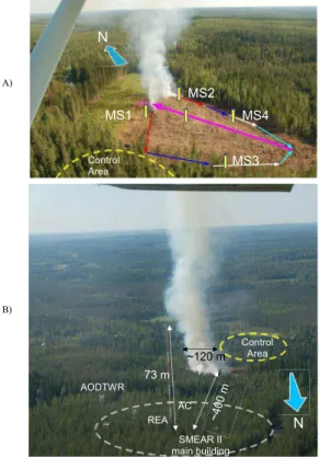
In addition to the burn area, we also selected a control site near the burning area (Fig. 1). At the burn site, there was a mature spruce-dominated stand with the stem volume per hectare of about 400 m3. The area was cut clear in February 2009. After

15

the clearcut most tree trunks were transported away; some of them and all tree tops and all branches were left on the ground in the burn area. An estimation of the biomass was done before and after the burning.

2.2 Estimation of burned organic material

The tree stand was measured in July 2008 from 13 relascope plots from which the

20

species, diameter at breast height (DBH), diameter at the height of 6.0 m, the living crown length and height (H) were recorded for each tree. Then, biomass models (Re-pola et al., 2007) were used to calculate the biomass for the di_fferent tree compo-nents. The merchantable wood was harvested in February 2009, after which all the non-merchantable trees were also felled. After burning the amount of unburned wood

25

(8)

ACPD

13, 21703–21763, 2013

experiment

A. Virkkula et al.

Title Page

Tables Figures

◭ ◮

Back Close

Full Screen / Esc

Discussion

P

a

per

|

D

iscussion

P

a

per

|

Discussion

P

a

per

|

Discuss

ion

P

a

per

|

(24 h, 105◦_{C) and weighted. The amount of burned tree biomass was finally calculated}

as an extraction of the merchantable tree biomass (tree tops, branches and non-merchantable trees) and unburned wood biomass. The surface vegetation, dominated by feather mosses and dwarf shrubs, was systematically sampled from 13 plots of 0.0625 m2in July–August. The vegetation was cut along the surface of the litter layer,

5

collected, dried (24 h, 105◦C) and weighed. The organic matter content of the upper-most, organic soil layers (litter layer and humus layer) was systematically sampled both before the clearcut in August 2008 and soon after the burning in July 2009. A total of 25 samples were collected on both occasions with a 45 mm-diameter soil auger. The samples were dried (24 h, 105◦_{C) and weighed. The mass of burned organic material}

10

in the organic soil layer was calculated as an extraction of the mass before and after the burning.

2.3 Gas, aerosol and meteorological measurements

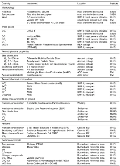
A list of the measurements conducted during the campaign is presented in Table 2. In short, trace gas concentrations, aerosol physical properties, aerosol chemical

compo-15

sition, and meteorological parameters were measured both at fixed sites and on mobile platforms.

2.3.1 Measurements at fixed positions

At the SMEAR II measurement station both aerosols and gases were measured with the setup described by Hari and Kulmala (2005). Measurements were conducted at

20

five di_fferent locations: the main building of the station, the 73-m-high SMEAR II mast, the aerosol cottage, the Relaxed Eddy Accumulation (REA) cottage, and the Aerosol Optical Depth Tower (AODTWR) about 100 m east of the aerosol cottage. The above measurements are within 300–400 m of the burn area (Fig. 1b).

The concentrations of CO₂, H₂O, O₃, NO, NO_x, SO₂ and CO were measured

con-25

(9)

ACPD

13, 21703–21763, 2013

experiment

A. Virkkula et al.

Title Page

Tables Figures

◭ ◮

Back Close

Full Screen / Esc

Discussion

P

a

per

|

D

iscussion

P

a

per

|

Discussion

P

a

per

|

Discuss

ion

P

a

per

main building and sample air was taken through six sample lines: PTFE Teflon™tubes, each 100 m long, and 14 or 16 mm in diameter. There was a continuous flow rate of 45 L min−1 _{in the lines, which resulted in an estimated lag time of 20 s. For each gas}

component, there was one analyser (a dual channel instrument for NO and NO_x) for measuring the concentrations. The response times of the analysers were about 30 s,

5

so, when sampling a new height, a flush time of about 30 s was needed. This set the signal recording time step to 1 min and the overall time spacing of the data to 6 min.

Volatile organic compounds (VOCs) were measured with Ionicon Analytik Proton Transfer Reaction Mass Spectrometers (PTR-MS, e.g., Hewitt et al., 2003) at two loca-tions: one at the SMEAR II main building with an inlet above the roof at about 10 m a.g.l.

10

and the other in the REA cottage with the inlet above canopy at the REA tower. The PTR-MS instrument measures charged VOCs at given mass that were assigned to the VOCs that likely dominated each signal. The assignment of mass-to-charge ratios (=m/z) to VOCs and the measurement setup is described by Taipale et al. (2008). Usually,m/z 69 is assigned to the biogenic VOCs isoprene and MBO, but, in this case,

15

m/z 69 was assigned to furan, which is associated with burning processes (de Gouw and Warneke, 2006). The VOC measurements were sampled every 1 min.

An Aerodyne Aerosol Mass Spectrometer (AMS) (e.g., Jayne et al., 2000; Jimenez et al., 2003; Drewnick et al., 2005) was used for measuring the concentrations of am-monium (NH+₄), sulfate (SO2₄−), nitrate (NO−₃), chloride (Cl−), and organics in particles

20

withD_p<600 nm. The AMS was located in the SMEAR II main building and it took its sample from the same inlet as the PTR-MS, above the roof at about 10 m a.g.l. The AMS measurements were taken every 5 min.

In the aerosol cottage, particle number size distributions for particles of 3–1000 nm in diameter were measured with a custom-made Twin-DMPS (TDMPS) system (Aalto

25

(10)

ACPD

13, 21703–21763, 2013

experiment

A. Virkkula et al.

Title Page

Tables Figures

◭ ◮

Back Close

Full Screen / Esc

Discussion

P

a

per

|

D

iscussion

P

a

per

|

Discussion

P

a

per

|

Discuss

ion

P

a

per

|

the mobility and size distributions of atmospheric ions and neutral clusters in the size range 0.8–47 nm (e.g., Manninen et al., 2009; Asmi et al., 2009) for the first time in a wildfire smoke plume. The NAIS measurements were taken every 2 min.

The aerosol optical measurements at SMEAR II were described in detail by Virkkula et al. (2011). In short, total scattering coe_fficients (σ_sp) and backscattering coe_fficients

5

(σ_bsp) were measured with a TSI 3λ nephelometer, averaged over a 5 min period. A Magee Scientific 7λ Aethalometer (AE-31) was used for measuring light absorp-tion, also at a 5 min averaging time. Absorption coe_fficient (σ_ap) was calculated from the aethalometer and nephelometer data using the algorithm by Arnott et al. (2005).

Aerosol optical depth was measured with a Cimel CE-318 sunphotometer in a tower

10

about 100 m east of the aerosol cottage (Fig. 1), above the canopy level. The sunpho-tometer made one instantaneous measurement every 15 min. In the same tower, light absorption coefficient at a wavelength (λ) of 637 nm was measured with a Multi-Angle Absorption Photometer (MAAP). The MAAP reports the absorption coe_fficient as black carbon concentrations using the mass absorption coe_fficient of 6.6 m2g−1_{. MAAP}

mea-15

surements were available every 1 min.

In addition to the SMEAR II measurements, we installed meteorological sensors on top of poles within and around the area to be burned. The poles were prepared by cutting the branches of five trees that were left standing in the slash. Four poles were outside the burning area, and one was within it (Fig. 1a). The distances of the poles 1, 2,

20

3, and 4 from the perimeter of the burn area were 10, 8, 9 and 6 m, respectively. In situ meteorological sensors (Vaisala WTX510) were deployed on the burn perimeter, and a sonic anemometer (ATI Sx-Probe) and Vaisala GMP-343 CO₂ sensor were placed within the burn area on the top of a pole at about 12 m in height. Total heat flux was measured at the surface with a water-cooled Hukseflux, Inc. SBG01 sensor.

25

2.3.2 Mobile measurements

(11)

ACPD

13, 21703–21763, 2013

experiment

A. Virkkula et al.

Title Page

Tables Figures

◭ ◮

Back Close

Full Screen / Esc

Discussion

P

a

per

|

D

iscussion

P

a

per

|

Discussion

P

a

per

|

Discuss

ion

P

a

per

was driven in the surrounding forest roads and stopped at several locations for some minutes. Sampling occurred above the windshield of the van at 2.4 m altitude. Particle number concentration and size distribution were measured by an Electrical Low Pres-sure Impactor (ELPI, Dekati Ltd) at a flow rate of 10 L min−1 (Keskinen et al., 1992). ELPI was equipped with a filter stage (Marjamäki et al., 2002) and a stage to enhance

5

the particle size resolution for nanoparticles (Yli-Ojanperä et al., 2010). The ELPI clas-sifies particles in the size range of 7 nm–10 µm (aerodynamic diameter) to 12 classes with samples every 1 s. Sniffer also monitored concentrations of CO, NO, NO₂ and CO₂at one-second intervals. Furthermore, PM_2.5and PM₁₀ were recorded by two TSI DustTrak aerosol monitors. A weather station on the roof ofSnifferat 2.9 m height

pro-10

vided meteorological parameters (temperature, relative humidity, wind speed and wind direction). A global positioning system (GPS) was used to record the van’s speed and the driving route.

In addition toSni_ffer, the dispersion on the ground level was measured by students walking around the area with three portable TSI model 3007 condensation particle

15

counters (CPCs) and GPS receivers. There were three different routes at three dis-tances from the burning area. The CPCs used in the nearest two routes were equipped with diluters because, according to the manual, the model 3007 CPC measures con-centrations up to 105cm−3. The diluters were calibrated afterwards and a flow rate of 0.7 L min−1_{in the 3007 CPC produced a dilution ratio of about 0.32. Thus, the}

concen-20

trations from the two nearest routes were divided by 0.32, resulting in the upper limit of the concentration range increasing to about 3×105cm−3.

Vertical and horizontal dispersion were measured with instruments installed in a Cessna 172, (Schobesberger et al., 2013). There were three CPCs for measuring particle number concentrations at three cutoffs (3, 6, and 10 nm). The 3 nm cutoffwas

25

(12)

Re-ACPD

13, 21703–21763, 2013

experiment

A. Virkkula et al.

Title Page

Tables Figures

◭ ◮

Back Close

Full Screen / Esc

Discussion

P

a

per

|

D

iscussion

P

a

per

|

Discussion

P

a

per

|

Discuss

ion

P

a

per

|

search model 903 nephelometer, and absorption coefficient (σap) was measured with

a Radiance Research 3-λParticle Soot Absorption Photometer (PSAP) atλ=467 nm, 530 nm, and 660 nm. A LICOR LI-84 measured CO₂ concentrations. The data were saved at 1-Hz frequency. The scattering and absorption coefficients will be discussed in the companion paper elsewhere.

5

2.3.3 Soil and flux measurements

The changes in soil physical, chemical and biological environment were monitored with a long-term perspective, as similar high frequency instrumentation described above for atmospheric aerosol and trace gas concentrations, are not available for the soil pa-rameters. Also, although the soil conditions do change rapidly during and after the fire,

10

many of the biological processes and responses to changing conditions have a lack-time, requiring several years of monitoring. These slowly changing responses were expected for instance in soil pH and the concentrations of available nitrogen, as well as soil greenhouse gas fluxes.

Long-term ecological measurements were begun in the mature forest in 2008 before

15

the clear cut and partial burning. The measurements were performed at three sites: (1) on the area that was later clear cut, (2) on the area that was later clear cut and also burned and (3) on an area that remained as a mature forest. These measurements comprised automatic soil temperature and moisture measurements in the organic layer and in the A and B mineral soil horizons, manual measurements of the heights of soil

20

organic layers, and the total carbon and nitrogen content, as well as available nitrogen species and pH in organic and mineral soil horizons. The soil horizon is a layer parallel to the soil surface, whose physical characteristics differ from the layers above and beneath. The measurement campaign ended in late 2011, two and half years after the burning

25

(13)

ACPD

13, 21703–21763, 2013

experiment

A. Virkkula et al.

Title Page

Tables Figures

◭ ◮

Back Close

Full Screen / Esc

Discussion

P

a

per

|

D

iscussion

P

a

per

|

Discussion

P

a

per

|

Discuss

ion

P

a

per

forest (Kulmala et al., 2012, 2013). The flux measurements were performed by plac-ing a chamber on a collar inserted approximately 5 cm within the soil. Eleven collars were inserted for CO₂ measurement and 8 collars were inserted for CH₄ measure-ment, respectively, at each site, and one closure took 4 min for CO₂ and 35 min for CH₄, as described in detail by Kulmala et al. (2013) and Pihlatie et al. (2013). During

5

2008–2010, CO₂fluxes at each site were also measured using an automatic chamber described in detail by Kulmala et al. (2010, 2011). We approximated the cumulative release of CO₂ after the treatments by interpolating the average e_ffluxes from each treatment separately.

The emission of forest-floor VOCs were measured five times at the burn site during

10

2008–2010. The VOC fluxes were measured on five permanently installed collars with a manual steady-state chamber system. The VOC sampling and analysis method is described by Aaltonen et al. (2011).

2.4 Formulas used for data processing

By using the measurements in the 12 m pole within the burning area, the turbulent

15

sensible heat flux was calculated from the covariance of the vertical velocity and sonic temperature perturbation as

H_s₌ρC_pw′_T′ ₍₁₎

where ρ is the air density, assumed to be constant, and Cp is the heat capacity of air at constant pressure. The turbulent kinetic energy (TKE) is the sum of the velocity

20

variances: TKE₌1

2

σu2+σv2+σw2

(14)

ACPD

13, 21703–21763, 2013

experiment

A. Virkkula et al.

Title Page

Tables Figures

◭ ◮

Back Close

Full Screen / Esc

Discussion

P

a

per

|

D

iscussion

P

a

per

|

Discussion

P

a

per

|

Discuss

ion

P

a

per

|

(= ∆CO₂) can be used for estimating the burning efficiency. The modified combustion (MCE) e_fficiency is defined as

MCE= ∆CO2

∆CO₂_{+ ∆}CO. (3)

MCE is often used as an indicator of whether the combustion is flaming or smoldering (e.g., Ward and Hao, 1992; Yokelson et al., 1996; Hobbs et al., 2003; van Leeuwen and

5

van der Werf, 2011).

The aerosol number size distributions were used for calculating volume size distribu-tions and the integrated mass concentradistribu-tions were calculated by assuming a density of 1.5 g cm−3_{. Three to five lognormal modes were fitted to the data up to 10 µm. The}

fitting yields the modal parameters (geometric mean diameter (D_g), geometric standard

10

deviation (σg), and number or volume concentration of the mode).

The in situ aerosol optical data were analyzed as discussed in Virkkula et al. (2011). Here we calculated three intensive aerosol optical properties: the single-scattering albedo (ω0), the Ångström exponent of scattering (αsp), and the backscatter fraction

(b).

15

ω₀= σsp

σsp+σap

(4)

is a measure of the darkness of aerosols: for purely scattering aerosols it equals 1 and for black carbon (BC) approximately 0.3_±0.1. The Ångström exponent of scattering α_sp describes the wavelength dependency of scattering and we calculated it for the nephelometer wavelength range by taking logarithm of scattering coefficients and the

20

respective wavelengths and fitting the data line to the line

ln(σ_sp)=−αspln(λ)+C (5)

(15)

ACPD

13, 21703–21763, 2013

experiment

A. Virkkula et al.

Title Page

Tables Figures

◭ ◮

Back Close

Full Screen / Esc

Discussion

P

a

per

|

D

iscussion

P

a

per

|

Discussion

P

a

per

|

Discuss

ion

P

a

per

particles. This relationship is not unambiguous, however (e.g., Schuster et al., 2006; Virkkula et al., 2011).

The backscatter fractionb

b=σ_σbsp

sp

(6)

whereσ_bsp is the backscattering coe_fficient, is a measure related to the angular

dis-5

tribution of light scattered by aerosol particles. From b it is possible to estimate the average upscatter fraction β and aerosol asymmetry parameter which are key prop-erties controlling the aerosol direct radiative forcing (e.g., Andrews et al., 2006). In general, larger particles scatter less light backwards than small particles so the size relationship ofbis qualitatively similar to that ofα_sp.

10

The radiative forcing e_fficiency (dF/δ), i.e., aerosol forcing per unit optical depth (δ) was calculated from:

∆F

δ =−DS0T

2

at(1−Ac)ω0β

(1₋R_s)2₋

₂_R s

β

1 ω₀

−1

(7)

whereD is the fractional day length, S₀ is the solar constant, T_at is the atmospheric transmission,A_c is the fractional cloud amount,R_sis the surface reflectance, andβis

15

the average upscatter fraction calculated fromb. If the non-aerosol-related factors are kept constant and if it is assumed thatβhas no zenith angle dependence this formula can be used for assessing the intrinsic radiative forcing efficiency by aerosols (e.g., Sheridan and Ogren, 1999; Delene and Ogren, 2002). The constants used wereD=

0.5, S₀₌1370 W m−2_,_T

at=0.76, Ac=0.6, and Rs=0.15 as suggested by Haywood

20

(16)

ACPD

13, 21703–21763, 2013

experiment

A. Virkkula et al.

Title Page

Tables Figures

◭ ◮

Back Close

Full Screen / Esc

Discussion

P

a

per

|

D

iscussion

P

a

per

|

Discussion

P

a

per

|

Discuss

ion

P

a

per

|

3 Results and discussion

3.1 General description of the burning

The measurement setup was ready at the beginning of May 2009, waiting for the wind to blow from the right direction (175–215◦_{) during dry conditions. In the morning of 26}

June wind was blowing from this direction and the sky was clear. A handheld smoke

5

signal was ignited soon after 07:00 East European Time (EET₌UTC₊2 h) in order to make the final decision of when to start the fire. The conditions were acceptable, so the area was set on fire at 07:45 EET. (All times presented below will be in EET, not in East European Summer Time.) The burning was performed against the wind as a broadcast burn; first the fire was ignited under the wind and then ignition slowly proceeded in both

10

directions (Fig. 1a). The idea was to slowly burn the edges of the site until a horseshoe-like shape was achieved and more than half of the area was burned. This phase of our experiment took about 110 min. Then, the edges were rapidly ignited in both directions over the wind so that the edges of the site were shut with the fire. Thereafter, the fire proceeded rapidly downwind, and flaming was over within about 25 min. The flaming

15

or active burning was over at 10:00 EET, and there was only a little visible smoke at 13:00 EET. These times will be shown in the figures below as the indicators of the flaming and smoldering phases of the burning, although the ends of both periods were not well defined. There were flames in some parts of the area while most of it was already smoldering, and smoldering biomass does not always emit visible smoke. For

20

the purposes of this paper, we define theplumeas approximately the visible column of smoke and thefire frontas the leading edge of the flames.

After the burning the amount of burned organic material was estimated as de-scribed above (Sect. 2.2). The amount of unburned wood was 30 700 kg. The burned area was approximately 0.81 ha so the amount of burned wood biomass

25

(17)

ACPD

13, 21703–21763, 2013

experiment

A. Virkkula et al.

Title Page

Tables Figures

◭ ◮

Back Close

Full Screen / Esc

Discussion

P

a

per

|

D

iscussion

P

a

per

|

Discussion

P

a

per

|

Discuss

ion

P

a

per

58 000 kg ha−1_{) was calculated as a sum of burned tree biomass, surface vegetation}

and organic soil layer (Table 1). Schlesinger (1991) noted that the carbon content of biomass is generally between 45 % and 50 % (by oven-dry mass). Table 1 also presents an estimated amount of carbon released by multiplying the biomass by 0.5.

3.2 Winds

5

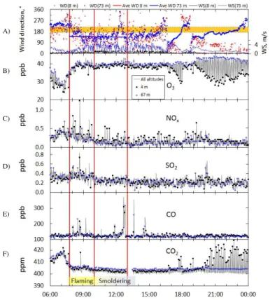
Most of the smoke ascended almost vertically, as seen from the aerial photographs taken during the flaming phase of the experiment (Fig. 1) indicating that wind speed was not high and no strong temperature inversion was present to inhibit the rising smoke. That the wind speed was low is also shown by measurements in the SMEAR II 73 m mast. At the ignition time, wind speed was<2 m s−1_{at all altitudes of the tower}

10

but it increased to 2–4 m s−1 _{during the morning (Fig. 2a). After ignition, the wind}

di-rection turned from southwesterly to southeasterly. On average, the didi-rectional shear between the 8.4 m and 73 m levels was small: the average wind direction was 138◦

and 134◦ _{at the 8.4 m level and 140}◦ _{and 136}◦ _{at the 73 m level during the flaming}

and smoldering phases, respectively. The average (±standard deviation) wind speed

15

was 0.55±0.26 m s−1 and 0.74±0.38 m s−1at the 8.4 m level and 2.2±1.1 m s−1and 3.0_±1.3 m s−1_{at the 73 m level during the flaming and smoldering phases, respectively.}

Measurements from the sonic anemometer at the top of the 12 m pole within the burning area (Fig. 3) show that both the wind direction and wind speed varied consid-erably more than at the SMEAR II mast. This is explainable both by the forest around

20

the high mast and by fire-induced winds within the open burning area. During the flam-ing period, the average wind direction and speed at the top of the pole were 189◦ _and

2.5_±1.1 m s−1_{(Fig. 3f and g) so the wind speed was slightly higher than at the top of}

the 73 m mast during the flaming period. The increased variability in wind speed and direction is caused by fire–atmosphere interactions that occur near the fire front and

25

(18)

wind-ACPD

13, 21703–21763, 2013

experiment

A. Virkkula et al.

Title Page

Tables Figures

◭ ◮

Back Close

Full Screen / Esc

Discussion

P

a

per

|

D

iscussion

P

a

per

|

Discussion

P

a

per

|

Discuss

ion

P

a

per

|

driven grass fires (Clements et al., 2007) and crown fires (Coen et al., 1999). Maximum updraft vertical velocities and maximum temperatures indicate the location of fire front (Clements et al., 2007).

Although the small-scale features of the fire front and variability in its intensity cannot be resolved by the vertical velocity and plume temperature (Fig. 3d and e), the crude,

5

near-surface properties of the atmosphere surrounding the combustion zone can be quantified. The fire front advanced from the northeast and northwest corners, south and around to the southern edge of the clearcut area. The fire burned as a head fire from the north to the south and through the center of the burn area. The fire was close to the mast several times, which is indicated by sharp increases in CO₂concentration,

10

positive vertical velocity (w) and temperature (T) (Fig. 3a, d and e). In addition, an abrupt change in wind direction also occurred during the fire-front passage (Fig. 3g). These observations of weak ambient winds, an upright plume, and higher fire intensity are consistent with plume-dominated fires (Sullivan, 2007).

The first fire-front passage occurred at 08:02–08:11 EET,T andwreached 59◦_{C and}

15

5.4 m s−1and the wind direction varied. The duration of the second plume passage was shorter (08:23–08:26 EET), followed by temperature increasing to a maximum of 84◦_C

and w increasing to 4.1 m s−1_{. The most pronounced fire-front passage occurred at}

08:35–08:52 EET whenT andwreached maximum values of 148◦C and 9.0 m s−1, the heat flux was in the range 20–40 kW m−2 _{(Fig. 3b), and the CO}

2concentrations were

20

in the range 2000–3000 ppm (Fig. 3a). This period is when the fire front passed under the instruments as indicated by the sharp increase in total heat flux (Fig. 3b). However, because there was no continuous video surveillance, it cannot be excluded that the above variations were from plume impinging on tower rather than fire underneath. After 09:02 EET, the area around the mast was burning more steadily but with a decreasing

25

intensity. At 09:03 EET,T andw maxima were 41◦_{C and 4.2 m s}−1_{, respectively, and at}

09:36 EET,T andw maxima were 26◦_{C and 2.5 m s}−1_{, respectively.}

(19)

ACPD

13, 21703–21763, 2013

experiment

A. Virkkula et al.

Title Page

Tables Figures

◭ ◮

Back Close

Full Screen / Esc

Discussion

P

a

per

|

D

iscussion

P

a

per

|

Discussion

P

a

per

|

Discuss

ion

P

a

per

fire-front passage. During the fire-front passage, the sensible heat flux increased to 20 kW m−2_{and peaked to}

∼58 kW m−2(Fig. 3b). Sharp increases inHsindicate when

the plume impinges on the mast and instrumentation, and sharp decreases in sensible heat flux indicate when the plume has passed and represent ambient conditions. The turbulent kinetic energy increased from approximately 1 m2s−2 _{before the plume and}

5

fire-front passage to nearly 15 m2s−2during the fire-front passage (Fig. 3c).

In addition to the pole in the middle of the burn area, four surface meteorological stations were deployed around the outside of the burn area (Fig. 1a). Although these surface stations did not experience the fire front directly as they were situated 6–10 m outside the burn area, they sampled the plume and the ambient meteorology

surround-10

ing the burn unit. The largest changes in meteorological measurements associated with the plume were collected by sensors 3 (southwest of the burn area) and 4 (southeast of the burn area). These two sensors recorded the more intense passage of the plume (13◦_{C and 18}◦_{C rises in temperature associated with the plume passage, respectively;}

Fig. 4a and b) than sensors 1 and 2 (4◦_{C and 2}◦_{C rises; not shown). The fire came}

15

closest to sensor 3 at about 09:10 EET and sampled the plume about 09:27–09:50 EET (Fig. 4a). The fire came closest to sensor 4 at about 09:15 EET and sampled the plume about 09:25–09:35 EET (Fig. 4b).

At sensor 3 around 09:27 EET, the wind shifted from southeasterly to southerly with a weakening wind of 1.5–2 m s−1_{(Fig. 4c). This shift was coincident with the beginning}

20

of a rise in temperature from 23◦_{C during which the wind shifted direction from}

south-easterly to southerly (Fig. 4a and c). By the time of the temperature peak of 35.8◦C at 09:35 EET, the relative humidity reached its minimum of 16.7 % with a slow drop over about the next 15 min (Fig. 4a).

In comparison, at sensor 4 around 09:21–09:24 EET, the wind shifted around to east

25

and northeast, suggesting that this is the inflow to the fire, and decreased (less than 1 m s−1_{, as low as 0.5 m s}−1_{) (Fig. 4d). A slow rise in temperature to 25}◦_{C followed}

(20)

ACPD

13, 21703–21763, 2013

experiment

A. Virkkula et al.

Title Page

Tables Figures

◭ ◮

Back Close

Full Screen / Esc

Discussion

P

a

per

|

D

iscussion

P

a

per

|

Discussion

P

a

per

|

Discuss

ion

P

a

per

|

52 % at the time of the most westerly wind (Fig. 4b and d) and the mixing ratio remained elevated (peaking at over 10 g kg−1 _{above an ambient value of 7–8 g kg}−1 _{when the}

plume was sampled). Interestingly, this sensor was the only one to record such a strong rise in relative humidity, perhaps because the sensor sampled the plume only about 10 min after its closest approach to the flames. Enhanced moisture in smoke plumes

5

due to combustion of wildland fuels has been suggested to possibly modify plume dynamics (Potter, 2005). Direct measurements of increased plume moisture have been made previously in grass fuels (Clements et al., 2006; Kiefer et al., 2012) with increase in water vapor mixing ratio of 1–3 g kg−1, and during smoldering fires in the longleaf-pine ecosystems in the southeastern United States (Achtemeier, 2006). During 09:25–

10

09:27 EET, the temperature rose to its peak (41.1◦_{C), and the RH decreased from 25–}

30 % to 16 % at the peak temperature (Fig. 4b).

3.3 Trace gases observations at the SMEAR II mast

The trace gases O₃, NO_x, SO₂, CO and CO₂, which are routinely measured at six diff er-ent altitudes in the mast, should all have clearly elevated concer-entrations in a biomass

15

burning plume (e.g., Radke et al., 1991). However, in the data from the mast, the con-centrations of most of them deviated very little from the background concon-centrations during the whole experiment (Fig. 2). The time series of trace gas concentrations mea-sured from the mast shows that the smoke plume arriving at the mast was narrow and patchy. The clearest concentration variations were for CO (Fig. 2e). During the

flam-20

ing phase, the highest CO concentration of 236 ppb was measured at 09:14 EET at an altitude of 33.6 m. This concentration was 127 ppb above the then-background value of 109 ppb, which was calculated as the running first percentile of the one-minute av-erages during the 30 min before and after each measurement. CO reached the peak value of 372 ppb, with the excess concentration_∆CO₌263 ppb during the smoldering

25

phase at 12:40 EET. The last two clear CO peaks were observed at 13:37 EET when

(21)

ACPD

13, 21703–21763, 2013

experiment

A. Virkkula et al.

Title Page

Tables Figures

◭ ◮

Back Close

Full Screen / Esc

Discussion

P

a

per

|

D

iscussion

P

a

per

|

Discussion

P

a

per

|

Discuss

ion

P

a

per

In complete combustion of hydrocarbon fuels in air, the reaction products include CO₂, water, and heat, in di_fferent proportions, and, in stoichiometric calculations, nitro-gen is also considered a reaction product (e.g., Flagan and Seinfeld, 1988). If, however, the burning process is incomplete, numerous other products are formed. The impor-tant products in the gas phase are CO and several condensable organic vapours. At

5

the high mast, the variations in CO₂concentrations were very small (Fig. 2f), suggest-ing that the smoke plume did not hit the mast. There was only one 1 min data point when it increased clearly above the baseline: at 08.47 EET, the CO₂ concentration peaked at 418 ppm. The then-running CO₂ baseline was 402 ppm, calculated as for CO above, so∆CO₂was 16 ppm. This peak occurred at the same time as a CO peak

10

with_∆CO₌62 ppb.

A scatterplot of ∆CO₂ vs.∆CO further confirms that their correlation was negligi-ble (Fig. 5a). The linear regression lines for ∆CO₂ vs. ∆CO were calculated for the data where_∆CO>40 ppb to examine whether even in the clearest plumes there was a positive relationship. There was a weak positive relationship. These regression lines

15

were used for estimating the emission ratio∆CO/∆CO₂. For instance during the flam-ing phase,_∆CO₂₌0.012×∆CO₊2.4 ppm, so when_∆CO₌100 ppb,_∆CO₂₌3.6 ppm and the ratio _∆CO/∆CO₂₌2.8 %. During the smoldering phase, the regression in Fig. 4 would yield ∆CO/∆CO₂=6.5 % at ∆CO=100 ppb. These ratios are consis-tent with some published values. For instance, Andreae and Merlet (2001) presented

20

the emission factors of several trace gases from various types of biomass burning. For extratropical forests, they give the emission factors for CO₂ of 1569±131 g kg−1 and for CO of 107±37 g kg−1 of burned dry biomass. From these numbers, the ratio

∆CO/∆CO₂₌6.8 % can be calculated at the mid value and the range from 4 % to 10 % by using the uncertainties.

25

(22)

ACPD

13, 21703–21763, 2013

experiment

A. Virkkula et al.

Title Page

Tables Figures

◭ ◮

Back Close

Full Screen / Esc

Discussion

P

a

per

|

D

iscussion

P

a

per

|

Discussion

P

a

per

|

Discuss

ion

P

a

per

|

flaming phase of the experiment, none of the MCEs were less than 0.9, but, during the smoldering phase, some of the MCE values were less than 0.9 and some were greater than 0.9 (Fig. 5b), roughly consistent with the previous results.

NO_x and SO₂, on the other hand, did have some peak concentrations above their baselines that correlated positively with_∆CO during the flaming phase (Fig. 5c and d).

5

The NO_x concentrations had peaks in times when no other indications of the smoke plume were present – for instance the three highest peaks during the smoldering phase. A probable explanation for these peaks is car tra_ffic around the station occurring during the burning.

The wind directions at the highest and lowest levels started to diverge gradually after

10

17:00 and in the period 21:00–midnight the di_fference was about 180◦_{. After 17:00 EET,}

8.4 m wind weakened and turned to the east-northeast (Fig. 2a), so the observed O₃ decrease and CO₂ increase at this level (Fig. 2b and f) were not related to possible emissions from the smoldering ground at the burned site, neither any of the SMEAR II ground-based aerosol measurements.

15

3.4 Aerosol at SMEAR II

3.4.1 Size distributions

The time series of aerosol number concentrations, the air ion and aerosol number size distributions, and the concentrations of organics show that even though wind blew from the right direction only for a short time, some distinct smoke peaks could be observed

20

at the aerosol cottage and at the SMEAR II main building where the AMS was operated (Fig. 6). Although the AMS measures the concentrations of organics, sulfate, nitrate, chloride, and ammonium, only the concentrations of organics increased in the plume. The concentration of BC measured with the Aethalometer increased above its baseline values only during the flaming phase (Fig. 6f). The peak 5 min average concentration of

25

3.4 µg m−3_{was measured at 08:07 EET. In the AOD tower above the canopy level, the}

(23)

ACPD

13, 21703–21763, 2013

experiment

A. Virkkula et al.

Title Page

Tables Figures

◭ ◮

Back Close

Full Screen / Esc

Discussion

P

a

per

|

D

iscussion

P

a

per

|

Discussion

P

a

per

|

Discuss

ion

P

a

per

In the plumes passing by the aerosol cottage during the smoldering phase, the BC concentrations did not increase at all; in the AOD tower, two 1 min peaks were detected (Fig. 6f).

The time series also shows one of the problems of the analysis. For instance, the sum of all species observed with the AMS is clearly lower than the mass

concentra-5

tion calculated from the number size distributions in the size rangeD_p<600 nm using a density of 1.5 g cm−3_{. In addition, some of the peak concentrations observed with the}

other aerosol instruments were not observed with the AMS at all (Fig. 6). The main reason is that the AMS and the DMPS were in different buildings, and the distance be-tween the two sites is about 100 m. In the case of a near-by smoke plume in low wind

10

speed conditions, the influence of this distance is significant.

The NAIS data show that cluster mode (D_p<2 nm) (Fig. 6e) and intermediate mode (D_p₌2–8 nm) (Fig. 6d) air ion number concentrations decreased significantly in the strongest smoke plumes, based on carbon monoxide and particle volume concentra-tions, both in the flaming and the smoldering phases, suggesting that the ions were

15

attached to the larger aerosols in the plume. The time series also shows that new particle formation occurred during the morning; at 09:20–09:50 EET, the cluster mode concentrations increased and there was a clear nucleation mode also in the size dis-tribution measured with the DMPS. At this time, all indicators of smoke plume were very low, wind was for a while blowing from the east at all levels (WD₌80–120◦_{) so the}

20

data suggest that the formation of new aerosol particles was natural and not due to the prescribed burning.

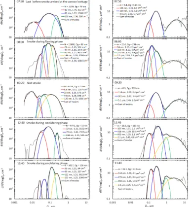
Particle number and volume size distributions were plotted for five selected times (Fig. 7). At 07:50 EET the smoke from the burning area had not yet reached the mea-surement station, so it can be as a representative of the “baseline size distribution”.

25

(24)

ACPD

13, 21703–21763, 2013

experiment

A. Virkkula et al.

Title Page

Tables Figures

◭ ◮

Back Close

Full Screen / Esc

Discussion

P

a

per

|

D

iscussion

P

a

per

|

Discussion

P

a

per

|

Discuss

ion

P

a

per

|

mode at 264 nm and a coarse mode at 3.6 µm. The integrated mass concentration was 9.4 µg m−3forD_p<10 µm.

The size distribution at 08:00 EET is the clearest one obtained from the smoke plume during the flaming phase. In the number size distribution, there were four modes, the largest of which was atD_g=80 nm. The geometric standard deviations, i.e., the widths

5

of the modes were quite small, ranging from 1.15 to 1.25 so the fitting was done also by assuming that instead of the three largest modes these comprise one large mode withD_g=81 nm, σ_g=1.58 (the dashed line at 08:00). In the volume size distribution there were four modes, the highest concentration of which was at atD_g₌153 nm. The integrated mass concentration was 21.6 µg m−3_{, the highest during the flaming phase.}

10

At 09:20 EET, there was a very clear nucleation mode at D_g=8.8 nm, simultane-ously with the high positive and negative air ion concentration in the sub-10 nm size range (Fig. 6). At this time, the number concentrations in the Aitken and accumulation modes were lower than in the smoke plume size distribution at 08:00 EET and not very different from those in the “background size distribution” at 07:50 EET, and the mass

15

concentration of 8.9 µg m−3was actually lower than at 07:50 EET. Therefore, it is rea-sonable to interpret this size distribution as representing natural new particle formation that is frequently observed at SMEAR II during sunny days (dal Maso et al., 2005).

The size distribution at 12:40 EET was measured from the thickest smoke plume ar-riving at the aerosol cottage during the smoldering phase. This time is when the CO

20

reached the maximum value (Fig. 2e), so the timing of these maxima suggests that this part of the otherwise very patchy plume was wide. In this size distribution, the integrated mass concentration of 28.6 µg m−3_{was the largest observed in the aerosol}

cottage during the experiment. In this number size distribution, the largest mode was at

D_g=79 nm, essentially at the same size as in the flaming-phase-plume size distribution

25

(25)

Sec-ACPD

13, 21703–21763, 2013

experiment

A. Virkkula et al.

Title Page

Tables Figures

◭ ◮

Back Close

Full Screen / Esc

Discussion

P

a

per

|

D

iscussion

P

a

per

|

Discussion

P

a

per

|

Discuss

ion

P

a

per

ond, in the smoldering-phase-plume volume size distribution, the contribution of the coarse-mode particles was much higher than in the flaming-phase-plume size distribu-tion. Actually, the broad shape of the supermicron size distribution and the highσ_g=2.4 suggest there were even more modes in the coarse sizes.

At 13:40 EET, another smoke plume was observed at the aerosol cottage, again

5

simultaneously with a CO peak in the mast. The number size distribution was more narrow with the largest mode at D_g=122 nm. The volume size distribution also had two clear accumulation modes and a broad coarse particle size distribution. The fast passage of the smoke plume creates uncertainty to the modal parameters since the smoke plume passages were shorter than the time used for scanning one size

distri-10

bution. Nevertheless, in both of the size distributions that were measured during the smoldering phase, the mass size distribution had much larger modes than during the flaming phase.

3.4.2 Aerosol optical characterization

In the first smoke plume observed during the flaming phase, light scattering coe_ffi

-15

cient (σ_sp) at λ=550 nm was 127 Mm−1 (Fig. 8). Because the mass concentrations obtained from the combined DMPS+APS data are available every 10 min, scattering data, which are available at 5 min intervals, were averaged over 10 min for comparison. The peak σ_sp in the first smoke plume passage was 93.8 Mm−1, whereas the mass concentration in the size rangeD_p<10 µm was 21.6 µg m−3_{(Fig. 7, volume size}

distri-20

bution at 08:00 EET), which yields a mass scattering efficiency of 4.3 m2g−1. The high-est 5 min-averaged σ_sp 137 Mm−1 _{was observed in the smoldering phase at the time}

the mass concentration reached the maximum value of 28.6 µg m−3(Fig. 7). The cor-responding 10 min-averagedσ_sp=116.5 Mm−1_{resulted in a mass scattering e}

fficiency of 4.1 m2g−1. These mass scattering efficiencies are somewhat higher than the value

25

(26)

ACPD

13, 21703–21763, 2013

experiment

A. Virkkula et al.

Title Page

Tables Figures

◭ ◮

Back Close

Full Screen / Esc

Discussion

P

a

per

|

D

iscussion

P

a

per

|

Discussion

P

a

per

|

Discuss

ion

P

a

per

|

et al., 2011), and the median value for the whole burning day that was also 3.1 m2g−1_,

but in good agreement with other published values (e.g., Malm and Hand, 2007). Light scattering increased when the smoke plume passed the aerosol cottage but the absorption coe_fficient increased only during two short periods in the flaming phase (Fig. 8a). This is somewhat strange because BC is one of the main products of

in-5

complete combustion. The aerosol was not very dark: the single-scattering albedω₀is about 0.3 for pure BC (e.g., Mikhailov et al., 2006) but during the experiment the lowest ω₀ was about 0.7 and in the strongest plume during the flaming phase 0.82. During the smoldering phaseω₀ was ≈0.9 and did not deviate from the background values during the smoke plumes (Fig. 8b).

10

In general the backscatter fractionbof larger particles is smaller than that of smaller particles so the size relationship of the backscatter fractionbis qualitatively similar to that of the Ångström exponent of scattering,α_sp. This was also observed in the smoke plumes. There were clear differences inα_spandbbetween the flaming and smoldering phases; both parameters were clearly lower in the smoke plumes observed during the

15

latter phase (Fig. 8). In the plumes during the flaming phase, the averageα_sp and b

were 2.25±0.01 and 0.171±0.001, respectively, and in the smoldering phase 1.56± 0.07 and 0.134±0.001, respectively. These observations and the higher contribution of coarse-mode particles in the smoldering phase (Fig. 7) than in the flaming phase are in line with the general picture of the size relationships of bothα_spandb. The two

20

parameters were especially well correlated during the smoldering phase (Fig. 9). The single-scattering albedo and the backscatter fraction were used for estimat-ing the radiative forcestimat-ing efficiency dF/δ from Eq. (7). dF/δ is negative for dark sur-face (R_s=0.15) both during the flaming and smoldering phases, even for the darkest aerosol during the flaming phase (Fig. 8d). ForR_s also the value of 0.85 was used to

25

(27)

ACPD

13, 21703–21763, 2013

experiment

A. Virkkula et al.

Title Page

Tables Figures

◭ ◮

Back Close

Full Screen / Esc

Discussion

P

a

per

|

D

iscussion

P

a

per

|

Discussion

P

a

per

|

Discuss

ion

P

a

per

To estimate the direct radiative forcing dF/δshould be multiplied by the aerosol op-tical depthδ. However, we do not have any measurement data on the smoke plume optical depth. The sunphotometer that was in the tower east of the aerosol cottage did not detect the smoke at all even though the MAAP that was at the same loca-tion did. The main reason is that the most of the smoke plume did not flow between

5

the sunphotometer and the Sun. Another reason is that the sunphotometer made one instantaneous measurement every 15 min according to AERONET (AErosol RObotic NETwork) settings and the smoke plume passed by the mast only during short 1–2 min periods (Fig. 6).

3.5 Organic trace gases

10

The time series of selected VOCs measured with PTR-MS at the two locations de-scribed in Sect. 2.3.1 are plotted together with the CO data from the mast in Fig. 10. The PTR-MS unit that operated in the REA cottage and took its sample from above the canopy sampled some of the clearest smoke plume passages during the flam-ing phase, but no data were available after 12:00 EET when the smoke plumes with

15

the high CO and aerosol mass concentration during the smoldering phase at 12:40– 12:50 EET were detected with the aerosol physical instruments. The unit at the SMEAR II main building that took its sample air from 10 m above ground level did not detect most of the plumes. This was probably caused partly by the unfavourable wind direc-tions in terms of their detection at this station, partly by the substantial meandering of

20

the smoke plumes. Below we only discuss the VOCs measured with the unit in the REA cottage.

Because CO provides the best evidence of burning among the trace gases, we com-pare it to the VOC data, even though they were not measured exactly at the same location. During the flaming phase there were three clear CO peaks detected in the

25