SRef-ID: 1607-7946/npg/2004-11-329
Nonlinear Processes
in Geophysics
© European Geosciences Union 2004
Second generation diffusion model of interacting gravity waves on
the surface of deep fluid
A. Pushkarev1,3, D. Resio2, and V. Zakharov1,3,4
1Waves and Solitons LLC, 918 W. Windsong Dr., Phoenix, AZ 85045, USA
2Coastal and Hydraulics Laboratory, U.S. Army Engineer Research and Development Center, Halls Ferry Road, Vicksburg,
MS 39180, USA
3Landau Institute for Theoretical Physics, Moscow, 117334, Russia
4Department of Mathematics, University of Arizona, Tucson, AZ 85721, USA
Received: 1 September 2003 – Revised: 22 January 2004 – Accepted: 2 June 2004 – Published: 27 July 2004
Abstract. We propose a second generation phenomeno-logical model for nonlinear interaction of gravity waves on the surface of deep water. This model takes into account the effects of non-locality of the original Hasselmann dif-fusion equation still preserving important properties of the first generation model: physically consistent scaling, adher-ence to conservation laws and the existadher-ence of Kolmogorov-Zakharov solutions. Numerical comparison of both models with the original Hasselmann equation shows that the second generation models improves the angular distribution in the evolving wave energy spectrum.
1 General theory
Forecasting wind waves is an important problem for oceanographers, coastal engineers, meteorologists and naval architects. It is widely accepted that the evolution of an ensemble of weakly nonlinear surface gravity waves is de-scribed by kinetic equation for waves. A simplified numer-ical solution of the kinetic equation (the discrete interac-tion approximainterac-tion) is, indeed, central to modern operainterac-tional wave-predicting models.
The kinetic equation for waves was first discovered by Nordheim (1928) (see also Pierls, 1981) in the context of solid state physics. Later on, this quantum-mechanical tool was applied to a wide variety of classical problems, includ-ing waves in plasma and hydrodynamics. Hasselmann (1962) and Zakharov and Filonenko (1966), Zakharov (1966) inde-pendently derived kinetic equation for surface waves from the original hydrodynamic equation
Correspondence to:A. Pushkarev ([email protected])
∂nk
∂t =Snl[n] (1)
Snl[n] =2πg2
Z
|Tk,k1,k2,k3|
2(n
k1nk2nk3+nknk2nk3
−nknk1nk2−nknk1nk3)δ(ωk+ωk1−ωk2−ωk3) δ(k+k1−k2−k3) dk1dk2dk3,
whereω=√gk.
Although, Hasselmann’s and Zakharov’s results differ in the general form of interaction coefficient, they become iden-tical, on the resonant surface (see Dyachenko and Lvov, 1995; Resio et al., 2001)
k+k1=k2+k3
ωk+ωk1 =ωk2+ωk3. (2)
It is important to recognize that that the meaning of func-tionnkin Hasselmann’s and Zakharov’s presentation is dif-ferent: “observable” wave action (Hasselmann) and “canon-ical” wave action (Zakharov). The details can be found in Zakharov (1999), here we just mention that the reason for appearance of the observable wave action in Hasselmann’s derivation consists in underestimation of “forced” harmon-ics. The difference between the observable and the canoni-cal wave action is small for physicanoni-cally important situations on deep water. In this paper we assume that the canonical and the observable wave action are identical. Equation (1) is known in oceanography as Hasselmann equation, or Snl
model. It formally conserves four integrals of motion: the wave actionN, the wave energyE, and two components of the momentumP:
N = Z
E= Z
ωknkdk (4)
P =
Z
knkdk (5)
The conservation of these quantities becomes obvious if Eq. (1) is rewritten in a differential form (see Zakharov, 2003).
Introducing polar coordinates(ω, φ)and supposing that
|k|=ωg2
Eq. (1) can be presented in the form ∂n
∂t = 1
ω3LˆAˆ[n], (6)
whereLˆ is the differential operator
ˆ
L= 1 2
∂2 ∂ω2 +
1 ω2
∂2
∂φ2 (7)
andAˆis the integral operator
ˆ
A[n] = ˆL−1ω3Snl. (8)
This operator has the form (see Appendix):
ˆ
A[n] = Z
A(ω, ω1, ω2, ω3, φ−φ1, φ−φ2, φ−φ3)
×n(ω1, φ1)n(ω2, φ2)n(ω3, φ3)dω1dω2dω3dφ1dφ2dφ3.
HereAis a complicated function homogeneous with respect toω-variables:
A(ǫω, ǫω1, ǫω2, ǫω3, φ−φ1, φ−φ2, φ−φ3)=
=ǫ21A(ω, ω1, ω2, ω3, φ−φ1, φ−φ2, φ−φ3) . (9)
Solutions of the stationary kinetic equation
Snl[n] =0 (10)
can be written in the form
ˆ
LAˆ[n] =0. (11)
Formally, thermodynamic solutions
n= T
ωk+µ
(12) satisfy the equation
ˆ
A[n] =0 (13)
but in reality, for functions like Eq. (12), the integrals inA diverge at largeω.
Solutions that are physically relevant satisfy the following equation:
ˆ
A[n] =P +Q ω+Mcosφ
ω . (14)
HereP andMare fluxes of energy and momentum to high wave numbers area andQis the flux of wave action to small wave number region. The general solution of Eqs. (13), (14) has to have, at k→∞, thermodynamical asymptotes to Eq. (12). However, due to the presence of dissipation at high wave numbers, one has to eliminate the thermodynamic asymptotes and put T→0 at k→∞. As a result, one can get a Kolmogorov-Zakharov (hereafterKZ) solution of the Eq. (14) in the form:
n(ω, φ)=g
10/3P1/3
ω8 F
ω Q
P , M ω P,cosφ
, (15)
while the energy spectrumǫ(ω, φ)can be expressed through n(ω, φ)as follows:
ǫ(ω, φ)= 2ω
4
g2 n(ω, φ) . (16)
Thus, the generalKZspectrum of energy is ǫ(ω, φ)= g
4/3P1/3
ω4 F
ω Q
P , M ω P,cosφ
. (17)
HereF is a dimensionless function of three variables to be determined numerically.
For the isotropic case we haveM=0 and the Kolmogorov solution is described by the function of one variable: ǫ(ω, φ)= g
4/3P1/3
ω4 H
ω Q
P
. (18)
Solution (18) presumes that there is a flux of energyP, di-rected to high wave numbers, together with a flux of wave ac-tionQis generated by external sources in this area. IfQ=0, Eq. (18) gives the simpleKZsolution: Zakharov-Filonenko spectrum (hereafterZF spectrum, (see Zakharov and Filo-nenko, 1966):
ǫ(ω, φ)=c0
g4/3P1/3
ω4 . (19)
FunctionH (ξ )has the asymptotic behavior:H (ξ )→q0ξ1/3
as ξ→∞. IfP=0, Eq. (18) gives another simpleKZ so-lution: Zakharov-Zaslavskii spectrum (Zakharov, 1966; Za-kharov and Zaslavskii, 1982):
ǫ(ω, φ)=q0
g4/3Q1/3
ω11/3 . (20)
IfQ=0, Eq. 18 describes a “pure” direct cascade governed by fluxes of energyP and momentumM:
ǫ(ω, φ)= g
4/3
ω4 P 1/3G
M
ω P,cosφ
. (21)
In the asymptotic area we haveM/ω P→0 and the spectrum takes the form
ǫ(ω, φ)= g
4/3
ω4 P 1/3
c0+
c1cosφ
ω + · · ·
, (22)
wherec0, c1are first and second Kolmogorov constants. All
2 Hasselmann-Iroshnikov model
Because the “exact” operatorAˆ[n]is very complicated, nu-merical solution of the non-stationary Eq. (6), as well as of the stationary form of Eq. (10) is quite complicated. Sev-eral simplified models of this operator have been attempted to date. The most popular one is so called DIA(Discrete Interaction Approximation), developed by Hasselmann et al. (1985). It is not our purpose to discuss theDIAmodel in this paper, since it has been the topic of considerable discussion in previous papers. Another approximation was simultane-ously and independently offered by Hasselmann and Has-selmann (1981) in somewhat different form by Iroshnikov (1985). They assumed that the coupling coefficientTkk1k2k3 is essential only if all the vectorsk, k1, k2, k3are close to each other (locality hypothesis).
Of course, there is no physical justification for such an as-sumption, but the mathematical model, adequate to this hy-pothesis, is interesting by itself. Hasselmann and Iroshnikov found that the assumption of locality presumes thatSnl is a
fourth-order nonlinear differential operator. Explicit forms of this operator are quite complex.
However, the explicit form of Hasselmann-Iroshnikov equation can be found by a unique way from very simple consideration Dyachenko et al. (1992). This equation has to conserve wave action, energy, and momentum; thus it has to be presented in the form of Eq. (6). SinceSnl is modeled by
fourth-order differential operator,Aˆhas to be a second-order operator. This operator has to be found uniquely from the requirement that Eq. (13) must have solutions of the form
n= P ω+µ
for any arbitraryP andµ. This requirement, together with the scaling property Eq. (1) implies
ˆ
A=a ω26n4L1
n. (23)
Finally, Eq. (1) takes the form ∂n
∂t = a
ω3L ω
26n4L1
n, (24)
whereais some constant. Stationary spectra in the differen-tial Hasselmann-Iroshnikov model satisfy the nonlinear el-liptic equation
n4 ∂
2
2∂ω2 +
1 ω2 ∂2 ∂φ2 ! 1 n =
P +ω Q+M cosφ/ω
c ω26 (25)
which must be solved numerically.
We should emphasize that Eq. (24) is a simplification of Eq. (1). It cannot be rigorously obtained from Hasselmann’s equation. Despite this fact, Eq. (24) reproduces all the basic properties of Eq. (1), i.e. it preserves all constants of motion and allows for the existence of bothKZand thermodynamic
spectra. All these solutions satisfy Eq. (25). The thermody-namic parametersT andµare defined by the asymptotic be-havior ofn(ω, φ)atω→∞. One can find an approximately “pure”KZsolution of Eq. (25) assuming that
n(ω, φ)= 1
ω8F (ω, φ), (26)
whereF (ω, φ)is a “slow function” of frequency. Within an accuracy of a few percent, we have
L1 n ≃ 28F ω2 and F ≃ 28 a 1/3
P +ω Q+M cosφ ω
1/3
. (27)
3 Local diffusion models
The fourth-order differential Eq. (24) is still a complicated approximation and is not convenient for analytical and nu-merical studies. To replace it, we propose a second-order nonlinear diffusion equation see Zakharov and Pushkarev (1999). In this very simple diffusion model, the complicated operatorAbecomes just a local algebraic expression
ˆ
A[n] =α1ω24n3, (28)
whereα1is some constant to be chosen empirically.
Now Eq. (1) can be written as the following nonlinear par-tial differenpar-tial equation:
∂n ∂t =
α1
ω3L nˆ 3ω24.
(29) This equation conserves basic constants of motion: wave ac-tion, energy, and momentum; it also maintains a full set of KZsolutions.
n(ω, φ)= 1 α11/3ω8
P +ω Q+M cosφ ω
1/3
. (30)
These solutions are close toKZsolutions for full differential Hasselmann-Iroshnikov model. We will call Eq. (29) Diffu-sion Model One (hereafterDE1). This equation has no ther-modynamic solutions. However, since wave spectra in nature are closer to a KZ form than to thermodynamic asymptotic forms, this is not a major problem.
TheDE1model was solved numerically by Zakharov and Pushkarev (1999) and by Polnikov and Farina (2002). It was proposed to consider the constantα1 in front of the
right-hand side of Eq. (29) as a special “tuning” constant to match the qualitative characteristics of theSnlmodel. The value of
this constant was chosen by comparison of numerical simula-tion of Eq. (29) with numerical simulasimula-tion of Eq. (1). Model DE1 reproduces several major properties ofSnl, such as: the
spectral peak down-shift and ZF power law nω∼ω−8. Its
4 Non-local diffusion models
The simple local diffusion modelDE1 has at least one major weak point. It predicts an angular spreading that is broader than that supported by experimental data. To improve this situation, we propose here two new diffusion models,DE2 andDE3. Both models are local in frequency but nonlocal with respect to angleφ:
model DE2:A=α2ω24n < n2>
model DE3:A=α3ω24n < n >2
where < n2>= 1
2π Z 2π
0
n2(ω, φ) dφ (31)
and < n >= 1
2π Z 2π
0
n(ω, φ) dφ . (32)
Equation (14), which definesKZspectra, can be easily solved by both nonlocal models. ForDE2this yields
n(ω, φ)= P
1/3
α1/32 ω8
1+ω QP + Mcosφ
P ω
1+ω QP 2+12 PM2ω22
4/3 (33)
and forDE3 n(ω, φ)= P
1/3
α1/33 ω8
1+ω QP +MP ωcosφ
1+ω QP
2/3 . (34)
Equations (33) and (34) display sharper dependence on the angle than Eq. (30). Let us mention that Eqs. (30), (33), (34) are valid only for frequencies ω>ωcrit. The ωcrit can be
found from equation P +ωcritQ=
M ωcrit
,
which yields
ωcrit=
p
P2+4M Q−P
2Q (35)
Ifω<ωcrit, spectra are negative in a certain sector ofω, φ
plane. To avoid this contradiction, one has to match Kol-mogorov spectra atω∼ωcrit either with a non-stationary
so-lution or with a stationary one with the presence of damping. To examine the characteristics of these three diffusion models, we performed the following steps:
1. Numerically computed the solution of the Cauchy prob-lem for theSnlmodel.
2. “Calibrated” the diffusion models (DE1, DE2, and DE3) for the Cauchy problem to determine the con-stants α1, α2, and α3, which provide the best
corre-spondence between time dependence of the total energy compared to the originalSnl.
3. Selected the best of the three models (DE1,DE2 and DE3) based on the comparison of the details of the en-ergy spectrum with the enen-ergy spectrum inSnlmodel.
4. Performed numerical tests with the “best” diffusion model to compare its characteristics with the corre-sponding ones obtained from numerical simulation of Snlmodel.
5 Calibration of theDE
As noted above, to calibrate different diffusion models, we solved numerically the same Cauchy problem for DE1, DE2, DE3 andSnl in the wind-driven case. We compare
our calculations with the results of numerical solution of the exact kinetic equation using a revised version of the Resio-Tracy code (Pushkarev et al., 2003).
The linear external source rateγ=γin+γdisswas chosen in the following manner. The wind input termγin(Donelan et al., 1985) was taken as
γin=2·10−4 ω
ω0−
1 2
ωcosθ,
−π/2< θ < π/2; ω0< ω < ω1 (36)
and the high-frequency dissipation term as γdiss = −D(ω−ω1)2,
ω1< ω < ωmax,
γdiss =0, ω < ω1. (37)
Here ω0=0.94 corresponds to wind velocity U≃10.4 m/s
andω1=8.48. High-frequency damping is used to simulate
infinite-capacity phase volume at high wave numbers. Con-stantD=−1.0 and frequencyω1are defined experimentally
from the condition of the effectiveness of the energy flux ab-sorption at high frequencies. We did not provide any damp-ing at small wave-numbers.
We found that constants α1=0.9·10−7
α2=1.8·10−7
α3=2.6·10−7 (38)
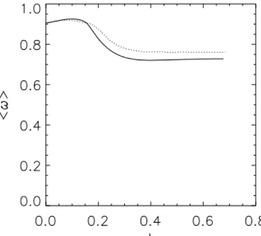
generated quite good correspondence in total energy behav-ior (see Fig. 1) and mean spectral frequency (see Fig. 2) as functions of time for all models.
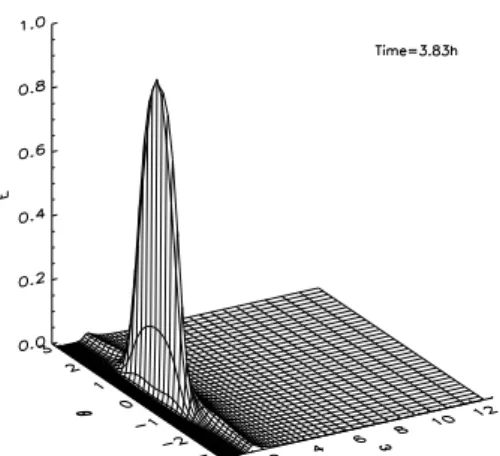
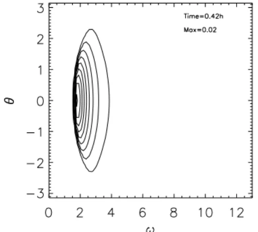
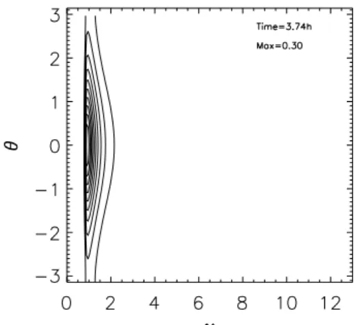
Figures 3–26 demonstrates the three-dimensional structure and line-levels of energy density for Snl, DE1, DE2 and
DE3 at three moments of time. All models demonstrate a growth in energy near the spectral peak along with a spectral peak down-shift and increased angular spreading away from the spectral peak. AllDE models exhibit lower spectrum maximum at the latest timet≃3.7 h, than the modelSnl.
can notice a significant deviation of the amplitude of the spectral maximum for modelSnl from corresponding values
in modelsDE. This deviation practically vanishes atω=1.0. This observation illustrates the following facts:
1. All DE models miss the “peakness” property of Snl
model (see Fig.27), while the correspondence improves away from the spectrum peak (see Fig. 28).
2. The distribution of energy is broader for theDEmodels than forSnl model (see Fig. 27).
Figure 28 also demonstrates that diffusion models DE2 and DE3 exhibit much closer correspondence in angular width withSnlmodel than the modelDE1.
Based on better correspondence in the angular width, we choose the modelsDE2 andDE3 as the best corresponding toSnl model. Since modelsDE2 andDE3 exhibit
practi-cally identical behavior, further discussion is based on the modelDE3.
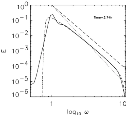
Figures 29–31 show the directional spectrum as a function ofω, and Figs. 32–34 show the logarithm of the directional spectrum as a function of logω for three times. One can see that correspondence betweenSnlandDE3 model is very
good everywhere, except in a narrow area near the spectral peak. The spectral tail exhibitsω−4behavior at all times of the simulation for both modelsSnlandDE3.
6 Testing of the “best” diffusion model
This section describes detailed comparison of theDE3 and Snl models. We performed this comparison for the
spe-cific “academic” choice of linear rates γin and γout (see Pushkarev et al., 2003). The reason is, it is not possible to reach complete equilibrium state for the situation with the wind input described in previous section – the spectral maximum continues to shift, though the rate of down-shifting dramatically diminishes.
To reach an actual equilibrium in this case, one has to in-troduce an artificial low-frequency damping, which stops the down-shift of the spectral maximum. We achieved that by choosing the following linear ratesγinandγout:
γin=D1e
−ω−ω0 0.19
4 − θ
π/4 8
if 0.63< ω <1.26 (39) and angular isotropic linear dissipation
γdiss=
−D2(ω−0.63)2ifω <0.63
−D3(ω−5.65)2ifω >5.65 . (40)
Here Di (i=1,2,3) are positive constants. Coefficient
D1=9.4·10−3 at Eq. (39) was defined from a condition of
smallness in the growth rate with respect to the correspond-ing local frequency. Negative components were chosen to represent the high and low frequency damping terms. They were introduced to absorb the direct (energy) and inverse (wave action) cascades. ConstantsD2=−1.andD3=−0.08
as well as frequenciesω=0.63 andω=5.65 were defined ex-perimentally from the following two conditions: effective-ness of the fluxes absorption and maximization of the inertial (forcing and damping free) interval with respect toω. Fig-ures 35, 36 show distribution of damping and instability de-fined by Eqs. (39), (40).
As in the previous section, we performed calibration by matching the time dependence of the total energy in DE3 andSnl models. The result of this match gave the value of
the constant
α3=2.2·10−7 (41)
Figures 37, 38 and 39 show the total energy, the average frequency and the energy flux as functions of time. It is quite obvious that these averages exhibit quite similar behavior in SnlandDE3 models.
Figure 40 shows the angle averaged energy density and cross-section of the energy density at zero angle for DE3 model. One can see that the angle-averaged spectrum behav-ior is close toω−4. The energy density along a cut at zero angle decays a little faster thanω−4, but still slower than ω−5. All these observations are in agreement with Eq. (22).
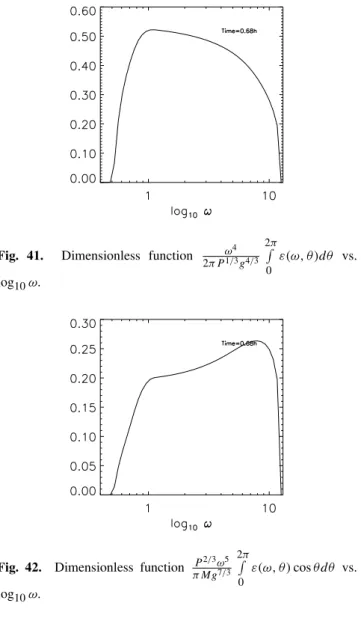
Figure 41 and Fig. 42 show the behavior of local values of the first and second Kolmogorov constantsC0 andC1(see
Pushkarev et al., 2003), calculated from the energy spectrum at the latest time of simulation for the modelDE3. One can estimate the value of the first Kolmogorov constant as
0.4< C0<0.5 (42)
and the value of the second Kolmogorov constant as
0.20< C1<0.26. (43)
These values are in good agreement with the values of Kol-mogorov constants measured forSnl model (see Pushkarev
et al., 2003)
0.33< C0<0.37 (44)
0.18< C1<0.27. (45)
7 Analytical properties ofDE3model
In our investigations we found that theDE2 andDE3 model were the most suitable models of all those tested here, at least in terms of reproducing relevant characteristics of spectral growth.
The equation ∂n
∂t = α3
ω3Lω
24Dn, D
=< n >2 (46)
present a solution of Eq. (43) in the form of Fourier series in angle
n(ω, θ, t )= ∞ X
n=−∞
Nn(ω, t )einθ
Nn=
1 2π
Z 2π
0
n(ω, θ, t )e−inωdθ (47)
NowD=N03.
InDE3 model,N0satisfies the closed equation
∂N0
∂t = α3
2ω3
∂2 ∂ω2ω
24N3
0 (48)
coinciding with DE1 equation for the radially-symmetric spectrum. Other coefficientsNnsatisfy the linear equations
∂Nn ∂t = α4 ω3 1 2 ∂2 ∂ω2 −
n2 ω2
!
ω24N02Nn. (49)
For large values ofnone can assume 1
2 ∂2 ∂ω2 ≪
n2
ω2. (50)
NowNnbehaves as follow
Nn≃e−α3n 2ω19Rt
0N02dt.
Assuming that in the stationary regimeN0≃α1p1/3/ω8, one
finds that the high angular harmonics vigorously decay in the high-frequency domain
Nn(t )≃e−α3N 2 0n2ω3t.
This consideration corroborates with the experimental fact of angular broadening of spectra in the high frequency region ω≫ωp.
The “conservative” (free of sources) Hasselmann kinetic equation has a two-parameter family of self-similar solutions (Zakharov, 2002). All the diffusive models have these so-lutions automatically. Since the only nonlinear equation in DE3 model matches the isotropic equation (48), this model is a convenient model for analytical studies of self-similar solutions. This a potentially important point and deserves future research.
In the presence of source terms, the variables in DE3 model do not separate any more. However, even in this case the use of the spectral code in angle looks very promising. We hope that on this way we would be able to speed up the computation times in order of magnitude in comparison with theDE1 model.
8 Conclusion
The diffusion approximation DE3 provides a good repro-duction of integral properties of Snl: the total energy, the
mean frequency, and the energy flux to high wave-numbers as functions of time. It also reproducesKZ spectra of en-ergy densityω−4and, after a proper optimization, the values of Kolmogorov constants.
This paper does not address the comparison of diffusive models with theDI Amodels. However, based on our exper-iments, we expect that their numerical performance should be comparable in efficiency. As far as both groups of mod-els are purely phenomenological, one could examine care-fully: which model better represents the spectral evolution described by the exact Snl equation. However, this is
be-yond the scope of this article and requires special investiga-tion which will be reported elsewhere.
The separation of variables in DE3 makes this model much more suitable for analytical study thanDE1. At the moment we use for the solution ofDE3 model the same nu-merical algorithm as for theDE1 model. Even in a frame-work of this approach, the DE3 model is 103 times faster than the exactSnl model, which can be very useful in
inves-tigations. Moreover, we believe that the use of spectral code in angle will make possible to speed up the code at least an order of magnitude.
TheDE3 model fails to reproduce the “peakness” prop-erty of Snl model; as a result DE3 exhibits lower values
of energy density at the spectral peak and a wider angular spread of energy in the vicinity of the spectral peak. How-ever, DE3 reproduces very well the angular spreading in the spectral region with frequencies greater than the spectral peak.
We are working on development of DE models to im-prove overall agreement with the full integral representation for spectral evolution.
Appendix
Operator A is expressed through Green function G(ω, ω′, φ) for the operator L. The Green function satisfies the equation
L G(ω, ω′, φ)=δ(ω−ω′) δ(φ)
G(0, ω′, φ)=0, G(∞, ω′, φ)=const. One can find
G(ω, ω′, φ)= − 1 2π ∞ X −∞ √ ωω′ 1n
einφ×
× " ω′ ω 1n Q
1−ω ′
ω
+ωω′1nQ ω′
ω −1 #
Fig. 1.Total energyEas the function of timet(hours). Solid line –Snl model, dotted line –DE1 model, dashed line –DE2 model, dash-dotted line –DE3 model.
Here 1n=
r 1 4+2n
2
and Q(ξ )=
1ξ >0 0ξ <0 OperatorAhas the form
A= 16π g4
Z
G(ω, ω′, φ−φ′)
×T (ω′, ω1, ω3, ω3, φ′−φ1, φ′−φ2, φ′−φ3)
2
×[n(ω1, φ1)n(ω2, φ2)n(ω3, φ3)
+n(ω′, φ′)n(ω2, φ2)n(ω3, φ3)
−n(ω′, φ′)n(ω1, φ1)n(ω2, φ2)
−n(ω′, φ′)n(ω1, φ1)n(ω3, φ3)δ(ω′+ω1−ω2−ω4)
δ(ω′2cosφ′+ω21cosφ1−ω22cosφ2−ω32cosφ3)
×δ(ω′2sinφ′+ω21sinφ1−ω22sinφ2−ω23sinφ3)
×ω′3ω13ω32ω33dω′dω1dω2dω3dφ′dφ1dφ2dφ3
EquationA[n]=0 has “formal” thermodynamic solutions
n= T
ω+p ω2cosφ+q ω2sinφ+µ
HereT,p,q, andµare constants.
Acknowledgements. The research presented in this paper was
conducted under ONR grant N00014-03-1-0648, US Army Corps of Engineers RDT&E program, grant DACW42-03-C-0019 and by NSF Grant NDMS0072803. This support is greatfully acknowl-edged.
Edited by: V. Shrira Reviewed by: one referee
Fig. 2. Average frequencyhωias the function of timet (hours). Solid line –Snl model, dotted line –DE1 model, dashed line – DE2 model, dash-dotted line –DE3 model.
Fig. 3.Energy density as a function of frequency and angle forSnl model.
Fig. 5.Energy density as a function of frequency and angle forSnl model.
Fig. 6.Energy density as a function of frequency and angle forSnl model.
Fig. 7.Energy density as a function of frequency and angle forSnl model.
Fig. 8.Energy density as a function of frequency and angle forSnl model.
Fig. 9. Energy density as a function of frequency and angle for DE1 model.
Fig. 11. Energy density as a function of frequency and angle for DE1 model.
Fig. 12. Energy density line levels as a function of frequency and angle forDE1 model.
Fig. 13. Energy density line levels as a function of frequency and angle forDE1 model.
Fig. 14. Energy density line levels as a function of frequency and angle forDE1 model.
Fig. 15. Energy density as a function of frequency and angle for DE2 model.
Fig. 17. Energy density as a function of frequency and angle for DE2 model.
Fig. 18. Energy density line levels as a function of frequency and angle forDE2 model.
Fig. 19. Energy density line levels as a function of frequency and angle forDE2 model.
Fig. 20. Energy density line levels as a function of frequency and angle forDE2 model.
Fig. 21. Energy density as a function of frequency and angle for DE3 model.
Fig. 23. Energy density as a function of frequency and angle for DE3 model.
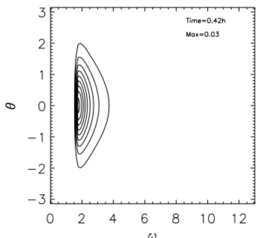
Fig. 24. Energy density line levels as a function of frequency and angle forDE3 model.
Fig. 25. Energy density line levels as a function of frequency and angle forDE3 model.
Fig. 26. Energy density line levels as a function of frequency and angle forDE3 model.
Fig. 27. Energy density cuts atω=1.0. Solid line –Snl model, dotted line –DE1 model, dashed line –DE2 model, dash-dotted line –DE3 model.
Fig. 29. Directional spectrum of the energy as a function ofω. ModelSnl– solid line, modelDE3 – dotted line.
Fig. 30. Directional spectrum of the energy as a function ofω. ModelSnl- solid line, modelDE3 – dotted line.
Fig. 31. Directional spectrum of the energy as a function ofω. ModelSnl– solid line, modelDE3 – dotted line.
Fig. 32. Decimal logarithm of the directional spectrum of the en-ergy as a function of the decimal logarithm ofωforSnlmodel (solid line) andDE3 model (dash-dotted line). Dashed line – function proportional toω−4, dotted line – function proportional toω−5.
Fig. 33. Decimal logarithm of the directional spectrum of the en-ergy as a function of the decimal logarithm ofωforSnlmodel (solid line) andDE3 model (dash-dotted line). Dashed line – function proportional toω−4, dotted line – function proportional toω−5.
Fig. 35.Linear growth rate as a function of frequency and angle.
Fig. 36. Linear growth rate line levels as a function of frequency and angle.
Fig. 37.Total energyEas the function of timet(hours). Solid line –Snlmodel, dotted line –DE3 model.
Fig. 38. Average frequencyhωias the function of timet(hours). Solid line –Snlmodel, dotted line –DE3 model.
Fig. 39. Energy flux as the function of timet(hours). Solid line – Snlmodel, dotted line –DE3 model.
Fig. 41. Dimensionless function ω4 2π P1/3g4/3
2π R
0
ε(ω, θ )dθ vs.
log10ω.
Fig. 42. Dimensionless function P2/3ω5 π Mg7/3
2π R
0
ε(ω, θ )cosθ dθ vs.
log10ω.
References
Donelan, M. A., Hamilton, J., and Hui, W. H.: Directional spectra of wind-generated waves, Phil. Trans. R. Soc. Lond., A315, 509– 562, 1985.
Dyachenko, A. I. and Lvov, Y. V.: On the Hasselmann and Zakharov approaches to the kinetic equations for gravity waves, J. Phys. Ocean., 25, 3227–3238, 1995.
Dyachenko S., Newell, A. C., Pushkarev, A., and Zakharov, V. E.: Optical turbulence: weak turbulence, condensates and collapsing filaments in the nonlinear Shroedinger equation, Physica D, 57, 96–100, 1992.
Hasselmann, K.: On the non-linear energy transfer in a gravity wave spectrum, Part 1, General theory., J. Fluid Mech., 12, 48, 1–500, 1962.
Hasselmann, S. and Hasselmann, K.: A symmetrical method of computing the nonlinear transfer in a gravity wave spectrum, Hamburger Geophys.Einzelschrift, 52, 138, 1981.
Hasselmann, S., Hasselmann, K., Allender, K. J., and Barnett, T. P.: Computations and parameterizations of the nonlinear energy transfer in a gravity-wave spectrum, Part II, J. Phys. Oceanogr., 15, 1378–1391, 1985.
Iroshnikov, R. S.: Possibility of a non-isotropic spectrum of wind waves by their weak nonlinear interaction, Sov. Phys. Dokl., 20, 126–128, 1985.
Nordheim, L. W.: On the kinetic method in the new statistics and its application in the electron theory of conductivity, Proc. R. Soc., A 119, 689–699, 1928.
Pierls, R.: Quantum theory of solids, Clarendon Press, Oxford, 1981.
Polnikov V. G., Farina, L.: On the problem of optimal approxima-tion of the four-wave kinetic integral, Nonl. Proc. Geophys., 20, 1–6, 2002.
Pushkarev, A., Resio, D., and Zakharov, V. E.: Weak turbulent ap-proach to the wind-generated gravity sea waves, Physica D: Non-linear Phenomena, Volume 184, Issue 1–4, 29-63, 2003. Resio, D., Pihl, J., Tracy, B., and Vincent, L.: Nonlinear energy
fluxes and the finite depth equilibrium range, J. Phys.Ocean., 106, C4, 6985–7000, 2001.
Zakharov, V. E.: Some aspects of nonlinear theory of surface waves (in Russian), PhD Thesis, Budker Institute for Nuclear Physics for Nuclear Physics, Novosibirsk, USSR, 1966.
Zakharov, V. E.: Statistical theory of gravity and capillary caves on the surface of a finite-depth fluid, Eur. J. Mech. B/Fluids, 18, 327–344, 1999.
Zakharov V. E.: Theoretical interpretation of fetch limited observa-tions of wind-driven sea, Preprints, 7th International Workshop on Wave Hindcasting and Forecasting, Banff, Alberta, Canada, October 21–25, 286–294, 2002.
Zakharov, V. E.: Direct and inverse cascades in wind-driven sea, J. Geophys. Res., in press, 2004.
Zakharov, V. E. and Filonenko, N. N.: Energy spectrum for stochas-tic oscillations of the surface of a fluid, Docl. Acad. Nauk SSSR, 160, 1292–1295, 1966.
Zakharov, V. E. and Zaslavskii, M. M.: The kinetic equation and Kolmogorov spectra in the weak turbulence theory of wind waves, Izv. Atm. Ocean. Phys., 18, 747–753, 1982.
Zakharov, V. E. and Pushkarev, A. N.: Diffusion model of inter-acting gravity waves on the surface of deep fluid, Nonlin. Proc. Geophys., 6, 1–10, 1999.