I
ZABELA
L
YON
F
REIRE
I
S THEM
ISMATCHN
EGATIVITY A SYMMETRICAL MEASURE OF CHANGE?
MATHEMATICO
-
PHILOSOPHICAL AND EXPERIMENTAL INVESTIGATIONS AIMED ATMAPPING PSYCHOTOPOLOGIES
Belo Horizonte
IZABELA LYON FREIRE
Is the Mismatch Negativity a symmetrical measure of
change?
mathematico-philosophical and experimental investigations
aimed at mapping psychotopologies
M. S. Thesis presented to the Universidade Federal de
Minas Gerais for the title of Master in Neuroscience
Concentration area: Psychophysics
Advisor: Prof. Dr. Hani Camille Yehia
Co-advisor: Prof. Dr. Carlos Julio Tierra-Criollo
Belo Horizonte
I hereby authorize complete or partial reproduction of this work, by any conventional or
electronic means, for study and research purposes, as long as the original source is properly
APPROVAL SHEET
Name: FREIRE, Izabela Lyon
Title: Is the Mismatch Negativity a symmetrical measure of change? Mathematico-philosophical
and experimental investigations aimed at mapping psychotopologies
M.S. Thesis presented to the Universidade Federal de
Minas Gerais for the title of Master in Neuroscience
Approved in:
Examing Committee
Prof. Dr. Hani Camille Yehia Institution: Universidade Federal de Minas Gerais
Judgement:__________________________ Signature:_______________________________
Prof. Dr. Carlos Julio Tierra-Criollo Institution: Universidade Federal de Minas Gerais
Judgement:__________________________ Signature:_______________________________
Prof. Dr. Maurício Alves Loureiro Institution: Universidade Federal de Minas Gerais
Judgement:__________________________ Signature:_______________________________
Prof. Dr Márcio Flávio Dutra Moraes Institution: Universidade Federal de Minas Gerais
R
ESUMO
FREIRE, IL. Será a Negatividade do desviante (Mismatch Negativity, MMN) uma medida simétrica de mudança? Investigações matemático-filosóficas e experimentais dirigidas ao
mapeamento de psicotopologias. Belo Horizonte. Departamento de Neurociências, Universidade
Federal de Minas Gerais, 2010. 58 p. Dissertação de Mestrado em Neurociências.
O potencial evocado conhecido como Negatividade do Desviante (Mismatch Negativity, MMN) é uma medida psicofísica de mudança discriminável. A forma mais simples de evocá-lo é através de experimentos no paradigma da bolota estranha no qual dois estímulos são apresentados em alternância aleatória: um deles acontecendo mais frequentemente, chamado de padrão, e outro acontecendo mais raramente, chamado de desviante. O MMN é a forma de onda calculada como a subtração da resposta ao padrão da resposta ao desviante. A literatura caracteriza o MMN como uma forma de onda cuja amplitude do pico aumenta e latência do pico diminui tanto com decrementos em probabilidade de apresentação do desviante quanto com a “diferença” entre estímulos utilizados nos papéis de padrão e desviante. Tal caractarização do MMN é em essência incompleta, já que não determina como fazer essa medida da “diferença” entre estímulos padrão e desviante, e as possibilidades de escolha de espaços métricos para o domínio dos estímulos físicos são várias. A literatura comumente assume que o MMN é uma medida simétrica de mudança e que uma reversão de papéis de padrão e desviante para os estímulos físicos utilizados no experimento da bolota estranha não afetaria a forma de onda do MMN. Diferenças observadas entre MMN’s obtidos no par de experimentos determinados pela troca de papéis são, na literatura, explicadas por diferenças em outros potenciais evocados sendo gravados durante o experimento. Este texto mostra que a hipótese de simetria do MMN é mal-definida, faltando-lhe rigor matemático, e propõe um paradigma experimental para a investigação da questão da simetria do MMN sob determinado espaço métrico para os estímulos físicos. Em termos experimentais, é demonstrado que o MMN para frequências se comporta de forma assimétrica sob a métrica “diferença absoluta, em Hertz, entre a frequência fundamental de tons complexos de três hamônicos”. Se for admitida a hipótese de que o MMN seja, em essência, uma medida simétrica de mudança, então a busca por espaços métricos para estímulos, sob os quais o MMN se comporte como tal, pode ser utilizada como ferramenta para o mapeamento da psicotopologia
do processamento daquele tipo de estímulo.
A
BSTRACT
FREIRE, IL Is the Mismatch Negativity a symmetrical measure of change? Mathematico-philosophical and experimental investigations aimed at mapping psychotopologies. Belo Horizonte. Neuroscience department, Universidade Federal de Minas Gerais, 2010. 58 p. Dissertação de Mestrado em Neurociências.
The event-related potential known as the Mismatch Negtivity (MMN) is a psychophysical measure of discriminable change. It is most simply evoked through experiments in the oddball paradigm, in which two stimuli are presented in random alternation, one more happening more frequently, thereby called the standard, and another more rarely, thereby called the deviant. The MMN is the waveform computed as the subtraction of the response to the standard from the response to the deviant. The literature characterizes the MMN as a waveform whose peak amplitude increases and peak latency decreases with decrements in the probability of presentation of deviant and with the “difference” between standard and deviant stimuli. This characterization of the MMN is in its essence incomplete, as it does not determine how to measure the “difference” between standard and deviant stimuli, and many metric spaces can be used for the domain of physical stimuli. The literature commonly assumes that the MMN is a symmetrical measure of change and that reversing roles of standard and deviant for the physical stimuli employed in the experiments will not affect the MMN. Differences observed between the MMN’s obtained in the pair of experiments determined by the swapping of roles have been explained by differences in other event-related potentials being recorded in the experiments. This work shows that the MMN symmetry assumption is ill-defined, lacking in mathematical rigour, and proposes an experimental framework for cleanly investigating whether the MMN behaves as a symmetrical measure of change under a given metric for the space of physical stimuli. Furthermore, experimental results for the frequency MMN, under the metric “absolute value of difference, in Hertz, between the fundamental frequency of three-harmonics complex tones”, are presented, and it is shown that, in this metric space for physical stimuli, the MMN is an asymmetrical measure of change. If it is assumed, a priori, that the MMN is a symmetrical measure of change, then searching for metric spaces for physical stimuli, under which the MMN behaves as such, can be used as a tool for mapping the psychotopology of processing that sort of stimuli.
L
IST OF ILLUSTRATIONS
Figure 2.1. Schematic illustration of auditory evoked potentials. Logarithmic scales are used for
amplitude and latency.
Figure 2.2. The “pure” MMN.
Figure 3.1. Schematic of the data collection environment.
Figure 4.1. Data collected from an experimental session lasting about 15 minutes (stimulus and EEG).
Figure 4.2. Zoom to 3 seconds of data shown in figure 5.1.1.
Figure 4.3. One-hundred consecutive single-trial recordings.
Table 4.1. Percentage of rejected epochs for each subject and round of experiments.
Table 4.2. Number of epochs of each type remaining after epoch rejection.
Figure 4.4. Grand-average waveforms.
Table 4.3. Amplitude and latencies for grand average waveforms shown in Figure 1.
Figure 4.5. ERP’s for each (tone, condition
Figure 4.6. cMMN.
Table 4.4. Comparison of latencies and amplitudes of cMMNsL and cMMNsH peak amplitudes and
latencies, in the per-(subject, round) average waveforms.
Figure 4.7. pMMN.
Table 4.5. Comparison of latencies and amplitudes of pMMNL and pMMNH peak amplitudes and
latencies, in the per-(subject, round) average waveforms.
Table 4.6. p-values and d’ for cMMN.
Table 4.7. p-values and d’ for pMMN.
Table 4.8. Re-sample analysis of characteristics of pMMNL compared to those of pMMNH.
Figure 5.1. Mel frequency scale.
Box 5.1. Text reproduced from (Kujala et al., 2007).
Box 5.2. How to calculate a ppMMN when using a distortion metric in φ.
Figure A.1. Validation of timing of stimulus delivery.
Box A.1. Matlab script for measuring inter-stimulus interval.
Figure A.2. ERP-like plots for each (tone, condition).
Figure A.3. cMMN-like plots. Akin to Figure 5.3.1.3, but data comes from a Balloon.
L
IST OF
S
YMBOLS AND DEFINITIONS
ϕ. Phi. The domain of physical events.
χ. Chi. In the Greek alphabet, χ comes right after ϕ and right before ψ. In this text it refers to the domain
of the Mismatch Negativity, overriding any traditional meaning.
ψ. Psi. The domain of mental events.
ℜ. The set of real numbers.
C(n, p). Number of different p-combinations of an n-element set. Its value is
C(n, p) =
Cnp = n!
(n−p)!p!
cMMN. “Classical” MMN, defined, in the oddball paradigm, as ERP for standard subtracted from ERP for deviant. Standards and deviants are presented within the same experimental block, in contrast against each other.
Cohen’s d. a.k.a. d’ (“d-prime”). Effect size measure, for quantifying the strength of the difference from
sample P1 to sample P2, with sample means µ1 and µ2, sample standard deviations σ1 and σ2, and sample
sizes n1 and n2. It measures the difference between the sample means in units of pooled standard
deviations:
, where
d’. See Cohen’s d.
Distance metric. A distance metric on a set X is a function M:X×X → ℜ, satisfying ∀x,y,z∈X, 1. d(x, y) ≥0 (non-negativity)
2. d(x, y) = 0 ⇔x = y (identity of indiscernibles) 3. d(x, y) = d(y, x) (symmetry)
4. d(x, z) ≥ d(x, y) + d(y, z) (triangle inequality)
If the third requirement (symmetry) is dropped (keeping 1, 2, and 4), then the function is called a distortion metric.
Distortion metric. See distance metric.
EEG. Electroencephalogram.
d'= µ1"µ2
#pooled
"pooled = (n1#1)"1
2
+(n2#1)"22
EMR. Electromagnetic radiation.
ERP. Event-related potential.
MMN. see cMMN.
N100. Negative-going ERP, peaking at 80-120 ms of stimulus onset. It is elicited by any unpredictable stimulus. Its amplitude shows refractoriness upon repetition of a stimulus. The use of a ramp of intensity
at tone onset decreases the N100 (Spreng 1980).
Oddball paradigm. Experimental paradigm in which two different stimuli are presented in random alternation. One of the stimuli happens significantly more rarely than the other and is thus called the
oddball, or deviant, while the other one is called the standard.
pMMN. “Pure” MMN, defined, in the oddball paradigm, as ERP for a stimulus φ1 presented as standard
minus ERP for that same φ1 presented as deviant. Two experimental blocks are required for computing a
pMMN. Probability of deviant should be the same in both blocks, as well as the numeriacal value of the metric function from standard to deviant.
pMMNH. The pMMN derived for the higher-frequency tone, in the oddball paradigm for frequency
MMN, assuming a distance metric in φ.
pMMNL. The pMMN derived for the lower-frequency tone, in the oddball paradigm for frequency MMN,
assuming a distance metric in φ.
ppMMN. A set of two MMN’s for which the numerical value of the metric function from standard to deviant is the same, as is the deviant probability.
T
ABLE OF
C
ONTENTS
Resumo ... 5
Abstract ... 6
List of Symbols and definitions ... 8
Introduction ... 12
Chapter 1. Psychophysics ... 15
Chapter 2. Background... 18
2.1. The electroencephalogram and event-related potentials ... 18
2.2. The Mismatch Negativity ... 19
2.2.1. A recent paradigm improvement for computing the Mismatch Negativity... 20
Chapter 3. Experimentation ... 22
3.1. Experimental sessions ... 22
3.1.1. Experimental subjects ... 22
3.1.2. Stimuli ... 22
3.1.3. The data collection environment ... 23
3.2. Signal processing... 25
3.3. Validation of experimental setup against artifactual data contamination ... 25
Chapter 4. Results ... 26
4.1. Streaming data ... 26
4.2. single trials ... 28
4.2.1. Examples of single trial data... 28
4.2.2. Results of data rejection procedures ... 28
4.3. Analysis of evoked potentials... 30
4.3.1. Averaged waveforms ... 30
Chapter 5. Discussion... 37
5.1. The analysis of experimental data ... 37
5.2. Published results on the effect of deviance direction on the MMN ... 38
5.3. Correctly interpreting pMMN’s ... 39
5.4. A novel, more rigorous formalization of the properties of the Mismatch Negativity... 44
5.4.1. Rigorously defining the assumption of symmetry of the MMN waveform to deviance direction... 44
5.4.2. A recent paradigm improvement for calculating the MMN, revisited: an experimental paradigm for measuring the pMMN under distortion metrics in φ... 47
5.4.3. Conclusions about the effect of deviance direction on the MMN waveform... 49
5.5. Further experiments in psychophysics of tone frequencies... 49
Chapter 6. Conclusions ... 50
6.1. Conclusions from experimental results ... 50
6.2. Conclusions about explanations available in the literature for differences in frequency pMMN’s ... 51
6.3. Conclusions from theoretical developments ... 51
References ... 52
Appendix. Validation of experimental environment... 55
A.1. Validation of timing of stimulus delivery ... 55
I
NTRODUCTION
This text is an exposition of experiments and theoretical work developed in the area of
psychophysics, which is, in general, aimed at understanding the relationship between physical
stimuli and psychological sensations. Measuring “psychological sensation” can only be done
indirectly, either through language, behavioral experiments, or physiological correlates.
Psychophysics is about measuring “psychological sensation” through physiological correlates,
from visible signs like the degree of dilation of pupils and presence of goosebumps, to quantities
requiring measurement machinery, like the conductivity of the skin, measured by a
galvanometer, or the timecourse of shifts in differences of potentials on the skull surface, which
reflect current dipoles inside the brain, and are measured by the electroencephalogram (EEG).
The last century has seen the popularization of EEG technology, and research with event related
potentials (ERP’s) has boomed. ERP’s are EEG waveforms that are related to current dipoles
involved in the processing of a triggering event, which may be exogenous, like a clarinet note, or
endogenous, like the imagination of the movement of a finger1.
The psychophysical measure taken as a tool for experimentation and also as an object of study in
itself is the Mismatch Negativity (MMN). The MMN is an ERP measure of discriminable
change, most simply evoked through experiments following the oddball paradigm, in which two
types of stimuli are presented in random alternation, one happening more frequently and another
happening more rarely. The MMN’s peak amplitude and latency parameters are functions of
stimulus unpredictability within a context, known to vary with both the probability and the
magnitude of change.
Experimental work was conducted in the auditory modality, with the frequency MMN, i.e., an
MMN evoked by differences in the frequency of the two types of stimuli utilized in the
experiment. The motivating question was: how is perception of magnitude of change related to
direction of change? That is, how is magnitude of change sensed when perceiving one extraneous stimulus, in the special case of this work, a G3 sinusoidal tone, among many
1
exemplars of another type of stimulus, here A4 sinusoidal tones, as compared to a situation in
which roles of the physical stimuli were swapped, that is, when A4 appears against a G3
background. The literature traditionally assumes that the MMN waveform will be the same in
both cases, and that any deviation from this would be due to contamination of the computed
MMN curve by other event-related potentials. A recent paper by Colin et al. (2009) found an
effect of direction of change in the MMN curve, utilizing duration MMN’s, and reports the
finding as a surprise:
The present report stems from observations made during a study of MMN parameters
across a wide range of duration contrasts. The data accumulated up to now strongly
suggested that there was an unanticipated systematic amplitude difference between
MMN’s evoked by shorter vs. longer deviants. The data analysis reported here was
performed in order to verify the serendipitous finding of an effect of deviance
direction on the MMN parameters, an issue that has hardly been addressed in the
literature.
Colin et al. (2009) offer an explanation to the effect they found, which is particular to the
duration MMN case2. In this dissertation, though, a different approach is taken to discussion of
the asymmetry of the MMN curve regarding deviance direction: in Chapter 3, a purely
theoretical study discusses how to define metrics in different spaces: the space of physical
stimuli,φ; the space of psychological sensations, ψ, and the space of the parameters of the MMN
waveform. As such, we conclude that defining a “reverse” experiment in which both the
probability of deviance and the metric from standard to deviant is kept the same, is not as simple
as switching which stimuli is in the role of a background, or standard, and which stimuli is in the
role of the foreground, or deviant, but depends on various assumptions about the nature of metric
spaces.
The text is organized as follows:
Chapter 1, Psychophysics, is a somewhat personal account on psychophysics. It is written in an informal style, like that of popular science books, with the occasional obscurely stated
reflections. In case the reader wishes to skip it, he will find that any concepts or nomenclature
2
thereby introduced, if needed for an understanding of the scientific work, have been soberly
catalogued in the List of Symbols.
Chapter 2, Background, discourses on electroencephalograms, event-related potentials, and, finally, the mismatch negativity (MMN).
Chapter 3, Experimentation, is a detailed description of the experimental work that was performed. It’s the arts & crafts, nuts & bolts, chapter.
Chapter 4, Results, is a description of the data obtained through the work described in the previous chapter.
Chapter 5, Discussion, reviews current MMN literature in light of the ideas hereby developed and of data presented in the previous chapter. In particular, section 5.4, A novel, more rigorous formalization of properties of the Mismatch Negativity, may be the most interesting contribution of the dissertation. Trying to apply mathematical rigour to an apparently
straightforward verbal construction utilized in the conceptualization of the MMN proposed by
Näätänen in 1990, and still widely accepted until today, gives rise to a few interesting
complications, to an improved paradigm for measuring the MMN, and to a
theoretically-determined critical discussion of some results from the published literature.
Chapter 6, Conclusions, enumerates conclusions drawn from the experimental work.
Appendix, Validation of experimental environment, presents demonstrations of the correct working of the experiments, including the balloon sessions, in which we tried to measure evoked
C
HAPTER
1.
P
SYCHOPHYSICS
According to (Gescheider, 1997), “psychophysics consists primarily of investigating the
relationships between sensations in the psychological domain ψ and stimuli in the physical
domain ϕ.”
The techniques for measuring events in ϕ are relatively well-developed, thanks to a
long-standing, well-justified obsession of physicists, expressed by Galileo Galilei as “Measure what
can be measured, and make measurable what cannot be measured.”
But would an expenditure of effort in trying to assess and measure events in ψ, through new
methodological and technological means, be justified? The uses would be many: understanding
communication by correlating mental events in ψ with characteristics in ϕ of communicative
acts; for neurology and psychiatry, establishing correlates in ϕ – either as causes or as
consequences – of mental states in ψ, or for evaluating the mental faculties of uncommunicative
patients, like those in a comatose state, or newborns; for criminalistics (recall the polygraph, aka
“lie detector”, incidentally but too amusingly celebrated in literature in the self-baptism of the
dog-turned-human Poligraf Poligrafovich Sharikov (Mikhail Bulgakov, Heart of a dog,
1925/1998)); for linguistics3; for an understanding of how various elements of music are
perceived, how music can be semantically interpreted and how it can exert such a deep effect on
people’s emotional states; and even back to physics: Henri Poincaré, in his (1905/2001) book On
the value of science, begins the chapter On the measure of time, with the sentence “So long as we
don’t go outside the domain of consciousness, the notion of time is relatively clear.”
That chapter of Poincaré has quite a few considerations on psychophysics, he even puts forth a
question about the sense of time, which has been extensively investigated through experiments
with evoked potentials (Jones 2002, Chen et al. 2010, Roger et al. 2009, Pulvermüller et al.
2006, etc)
3
Can we transform psychologic time, which is qualitative, into a quantitative time? […]
This difficulty has long been noticed; it has been the subject of long discussions and
one may say the question is settled. We have not a direct intuition of the equality of
two intervals of time. The persons who believe they posses this intuition are dupes of
an illusion. When I say, from noon to one the same time passes as from two to three,
what meaning has this affirmation? (Poincaré, 1905).
Lastly, the relationship between the domains ψ and ϕ is one of the grails of philosophy.
Quantifying events in ψ is not always easy4 – but it’s often tempting. Let’s delay the text about
the perception of differences in piano tones, from G3 to A4, versus in the opposite direction from
A4 to G3, to the next section, as ψ and ϕ can be so much more than that. For now, take love: in
which sense could the difference between the love of one couple and that of another be only
quantitative, a matter of which and how many adverbs, in which order, are chained between the
words “I love you” and “much”? This silly idea probably calls for some sort of decomposition of
“love” into components, but, the bottom question is, could such things ultimately be measured?
What is measured by the exact frequency and angle at which a german shepherd wags her tail5,
by the exact frequency, speed and pressure employed when she licks your face, or how
watchfully she behaves from far away whenever a stranger approaches you: how quietly she
holds her breath (with the tip of her tongue dangling out of her quasi-closed mouth), how fixedly
she stares, and how sharply she points her ears; what if that happens p% of the times a stranger
comes near, and in the other (100 – p)% she does not take notice because she is busy with
something else? What is measured by your reaction time for jumping after that dog when she’s a
meter away from a coiled snake, catching her in your arms and jumping away? Aren’t those
numbers enough to measure the love6? More directly, Umberto Eco, in The name of the rose
(1980/1983), cites Avicenna, the Persian sage, and Galen, the Roman physician:
Avicenna advised an infallible method already proposed by Galen for discovering
whether someone is in love: grasp the wrist of the sufferer and utter many names of
4 Oh and who can we turn to in this need? Not angels not people and the cunning animals realize at once that we aren’t especially at home in the deciphered world (Rainer Maria Rilke, Duino Elegies, (1912/2006))
5 As a matter of fact, dogs wag their whole body.
members of the opposite sex, until you discover which name makes the pulse
accelerate.
so a function of rate of heartbeat, in ϕ, would be a measure of love, in ψ, and the manner
advocated to take that measure would be through language. That is psychophysics as well!
A famous example is Libet’s (1999) event-related potential study of free will.
An interesting question to be posed once one decides that some of the more abstract members of
ψ can be quantified, would be: what’s the interplay of the quantitative and the qualitative in the
domain of ψ? Could important qualitative changes occur in ψ upon reaching quantitative
thresholds? An example of such is described in Milan Kundera’s Eduard and God (1969/1999):
Eduard is sitting in a wooden pew and feeling sad at the thought that God does not
exist. But just at this moment his sadness is so great that suddenly from its depth
emerges the genuine living face of God. Look! It's true! Eduard is smiling! He is
smiling, and his smile is happy. Please keep him in your memory with this smile.
But… this is too far gone on thoughts on quantities, measurements, ψ, qualitative transitions,
even God, ϕ, magnitudes of feelings, Olympics with babies, snakes, far-away olfactory feats, and
what not, pardon me and my digressions on psychophysics: the real problem now is that the rest
of this thesis is going to be mind-numbingly boring, and at points irritating, except for a minorly
amusing corollary about the absence of event-related potentials in balloons, which was based on
necessary work to prove that we were actually measuring evoked potentials instead of artifactual
noise. Evoked potentials are hard to measure, because their magnitude is on the order of µvolts,
and it was a lot of work to make sure that all the equipment was functioning properly. The grey
balloon sessions were left for an Appendix. The rest of the text is about the correct manner of
measuring the workings of a neural system that is considered an EEG correlate of discriminable
change, outputting an EEG waveform that peaks within 90 to 200 ms of change onset, the
C
HAPTER
2.
B
ACKGROUND
2.1.
T
HE ELECTROENCEPHALOGRAM AND EVENT-
RELATED POTENTIALS7Electrical currents in the brain are associated with net differences of potential on the skull
surface. Measurements of these differences of potential over time make up the
electroencephalogram (EEG).
The first EEG was measured in 1875, on the exposed cortex of rabbits and monkeys, by Richard
Caton, in England. Caton was able to observe both spontaneous electrical activity and sensory
event-related potentials (ERP’s)(Swartz and Goldensohn, 1998).
An ERP to a triggering event e is the set of changes in the EEG that are caused by e. The
timecourse of known ERP’s is on scales of tens to hundreds of milliseconds.
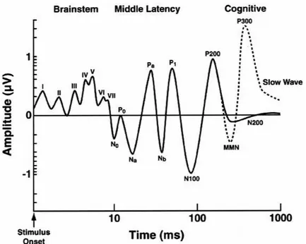
A schematic illustration of auditory ERP’s is shown in Figure 2.1: in the first 10ms following
stimulus onset, very specific waveforms are drawn in the EEG due to currents flowing at the
brainstem level; in the other end of the time and hierarchy of processing spectrum, the P300
appears, with latencies of more than 300 ms of stimulus onset, as an EEG correlate of processing
of a rare, task-relevant stimulus (Duncan et al., 2009). Brainstem-level ERP’s are naturally easier
to discover and characterize. It’s interesting, though, that current research has identified cortical
responses like the N400. The N400 exists in the domain of language processing, and its
amplitude is correlated with how surprising is the appearance of a word in a given context! (Lau
et al., 2008).
One is urged to notice that the voltage fluctuations between certain pairs of points on the skull
surface draw very particular EEG waveforms in response to certain events, upon repetition of
events in this class to an experimental subject and even across different subjects. This is not
shocking if one considers the current state of knowledge of functional neuroanatomy, with
precise localization of some functions to known brain structures, especially of lower-level
functions in sensory processing. For the justifiably skeptical reader, the inter-subject stability and
test-retest replicability of auditory event-related potentials N1 and P2 have been demonstrated in
Roth et al., (1975) and Shelley et al. (1991).
Figure 2.1. Schematic illustration of auditory evoked potentials. Logarithmic scales are used
for amplitude and latency. Figure extracted from Picton et al. (1974).
ERP changes are of course embedded in the overall spontaneous activity of the brain. EEG
differences of potential, when measured on the skull surface, are on the order of hundreds of
millivolts, while ERP’s are on the order of a few microvolts. This makes appropriate
experimental design and signal processing techniques necessary to isolate ERP’s from other
activity being measured in the EEG. The most common modus operandi of ERP research
nowadays is experimental design based on repeated presentation of the stimulus that triggers the
ERP and signal processing by time-locked, stimulus-synchronized, EEG averaging to cancel out
non-specific brain activity. Other issues are involved, mainly regarding data de-noising, but such
are peripheral to the basic understanding of the concept and will not be discussed here. A good
introductory book on ERP research is (Luck, 2005).
2.2.
T
HEM
ISMATCHN
EGATIVITYThe Mismatch Negativity (MMN) is an event-related potential whose latency and amplitude
measures of the brain’s response to violations of a rule, established by a sequence of sensory
stimuli (Näätänen, 1992). The MMN can be most simply evoked through the oddball paradigm,
in which standard and deviant stimuli are presented in random alternation, with the probability
of presentation of standard being higher than that for the deviant. One example of experimental
design following the oddball paradigm is presentation of randomly alternating middle C and
middle F piano tones, each occurring with probabilities 85 and 15%, respectively. The MMN
would then be defined as the subtraction of the potential evoked by the C tone from the potential
evoked by the F tone. The waveform peaks between 90 and 200 ms after stimulus onset,
depending on the type of regularity that is broken, and lasts between 80 and 200 ms (Kujala et
al., 2007).
The MMN was discovered in 1978 at the Institute for Perception, TNO, The Netherlands
(Näätänen, Gaillard, Mantysalo, 1978). As of February 14th, 2010, a Pubmed search for
“mismatch negativity” retrieves 1264 articles, spanning diverse research and application areas
such as sensory processing, clinical neurology and psychiatry, linguistics, phonoaudiology,
neuropharmacology, and memory and attention functions.
In Näätänen (1990, 1992), the folllowing properties are given for the MMN:
I. The smaller the probability of occurrence of the deviant within the sound sequence, the larger
the MMN's amplitude.
II. The larger the difference between deviant and standard stimuli, the larger the MMN's
amplitude, and the shorter its peak latency.
III. The MMN is elicited whether the subjects are instructed to detect the deviant sounds or are
engaged in a neutral primary task (e.g., reading a book). In the first case, though, the
waveform is overlapped by attention- and task-dependent components, such as the P165 and
the N2b (see, e.g., Sams, Paavilainen, Alho, & Näätänen, 1985).
Interestingly, the MMN appears also for violations of abstract rules, like “the higher the
frequency of a stimulus, the louder its intensity”, and, as such, it must rely on mechanisms for
detecting this sort of perceptual invariance (Paavilainen et al., 2003).
2.2.1. A RECENT PARADIGM IMPROVEMENT FOR COMPUTING THE MISMATCH NEGATIVITY
This subsection explains a paradigm aimed at better measuring the MMN, presented in (Kujala et
al., (2007)8,9. Special mention is made of this idea because it’s a seed for the developments made
in the work presented in this dissertation.
8
The paradigm aims at eliminating, from the MMN curve, the non-MMN effects that are due to
different physical characteristics of standard and deviant stimuli. In an oddball paradigm
experiment, in which physical stimuli φ1 and φ2 are presented, respectively, as standard and
deviant, with deviant probability p, one subtracts from the ERP to φ1 presented as deviant, not
the ERP to φ2 presented as standard, as is classically done, but an ERP to φ1 presented as
standard. There are two options for choice of this last mentioned ERP: either take an ERP to φ1
presented by itself, or an ERP to φ1 presented as standard against φ1 presented as deviant with
probability p (i.e., run an experiment in the oddball paradigm in which standard/deviant roles for
φ1 and φ2 are reversed). The MMN calculated in this manner will be called a pure MMN, or
pMMN. In the second approach, two pMMN’s are obtained, and collectively called a pair of
pMMN’s, or ppMMN. The second approach is illustrated in Figure 2.2.
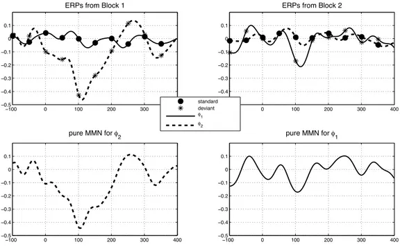
Figure 2.2. The “pure” MMN. In block 1, φ1 is presented as deviant and φ2 is presented as
standard. In block 2, roles are reversed. ERP’s derived during presentation of φ
1 are drawn in
broken lines, and, during presentation of φ
2, in full lines. Standards are marked ‘o’ and deviants
are marked ‘*’. A “pure” MMN is calculated as the subtraction of ERP for φi presented as
standard from ERP for φi presented as deviant. Deviant probability is the same in both blocks.
The figure shows real data obtained in our lab with the frequency MMN.
9
The text from the relevant section of (Kujala et al., 2007) has been transcribed in Box 5.2 of this dissertation.
!!"" " !"" #"" $"" %""
!"&' !"&% !"&$ !"&# !"&! " "&! ()*+,-./0,12/34,!
!!"" " !"" #"" $"" %""
!"&' !"&% !"&$ !"&# !"&! " "&! ()*+,-./0,12/34,# , , +56786.8 89:;675 !! !#
!!"" " !"" #"" $"" %""
!"&' !"&% !"&$ !"&# !"&! " "&! <=.9,>>?,-/.,! #
!!"" " !"" #"" $"" %""
C
HAPTER
3.
E
XPERIMENTATION
This chapter describes all aspects of the experimental work: from creation of stimuli to the set up
of the data recording environment and signal processing techniques.
Closely related to this chapter is the Appendix, which provides a demonstration of absence of
data contamination by experimental artifacts: all procedures were repeated on an inflated balloon
in the place of a live-brain-filled skull. Artifacts can lurk in from unexpected sources.
3.1.
E
XPERIMENTAL SESSIONS3.1.1. EXPERIMENTAL SUBJECTS
EEG data was collected from 7 adult subjects, aged between 20 and 30 years old, recruited
among graduate students at UFMG. None of the subjects was ever diagnosed with any auditive,
neurological, or psychiatric disorder, neither made use of any medicament that could interfere
with the generalization of the results to a healthy population. The subjects were naïve about the
purpose of the study.
3.1.2. STIMULI
Stimuli were 200 ms tones of 196.0 Hz (called t0 from now on) and 466.2 Hz (called t1 from
now on), each added of their first two harmonics, with linear onset and offset ramps of 10
milliseconds each. Choice of fundamental frequencies was based on Fujioka, Trainor and Ross,
(2008), and the use of complex tones with extra harmonic was based on Jones, (2002) and
Novitski et al., (2004). Harmonical tones elicit MMN with shorter latencies and larger
amplitudes than do pure sinusoidal tones. Stimulus onset asynchrony (SOA) was 500
milliseconds. Probability of deviant was 15%, and deviants were presented in random order,
under the condition that no two consecutive deviants were allowed. 1800 trials were run in each
round, and in-between rounds there was a period of one minute of silence. For 3 of the subjects,
2 rounds were presented: in the first round, the standard was the 196 Hz tone, and the deviant
was the 466.2 Hz tone. In the second round, roles were reversed. For 4 of the subjects, a third
round was presented which exactly reproduced the first round. The sequence of standards and
deviants was the same in all rounds, what varied was only which tone was allocated to the role of
be introduced due to ordering of presentation. Stimuli were played as .wav files by iTunes 9.0.2
software on a MacBook running 10.5.8 OS X. The method of stimulus delivery was shown to
yield accurate timing. The demonstration is described in the Appendix.
3.1.3. THE DATA COLLECTION ENVIRONMENT
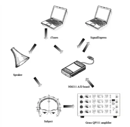
A schematic of the wiring of machinery for data collection is shown in Figure 3.1.
Figure 3.1. Schematic of the data collection environment. Subject’s head should be kept as
far as possible from all power cables and electronics. The speaker and amplifier utilized A/C power, all other machinery utilized D/C power. Regardless of utilizing A/C or D/C power, computer monitors can emit significant electromagnetic radiation (EMR) at the screen refresh ratio. Headphones can be a source of EMR as well, and the utilization of a speaker provides a solution to this problem, which is made more convenient if performing the experiments in an acoustically shielded room. Before running each experiment, it’s a good idea to check proper
functioning of machinery by briefly displaying cardiac signals on the live screen10.
Voltage was measured between Fz (that is, at one-third of the shortest path on the skull surface
from nasion to inion) and the right mastoid, using a Grass QP511 amplifier system. Ground
potential was established at the subject's forehead. Analog filtering was performed in the QP511
system, with band-pass filtering between 0.1 and 100 Hz and line filter at 60 Hz. Signal was
amplified by a factor of 50K. The amplifier system's power was supplied by the building's power
lines.
Measurements were made using gold electrodes after skin cleansing (with alcohol). Conductive
paste was applied between the electrodes and the skin. The subject was kept at least one meter
away from any electricity-conducting cable or working electric equipment, such as the laptops or
the amplifier system.
Experiments were run in an acoustically shielded room. Stimuli were delivered by speakers
placed 1.5 meters away from subject's ears; sound intensity at the ears was 70dB SPL. Subjects
were instructed to lie down, relax and listen passively to the stimuli with their eyes open. Light
intensity was kept low.
Analog-to-digital conversion was performed by a National Instruments NI6211 acquisition
board, and controlled by the software NI LabVIEW SignalExpress, running on a Windows Vista
laptop. The power to the acquisition board was supplied via a USB cable connected to this same
laptop. The laptop was run on batteries. The acquisition board was configured to sample the
signal at 1kHz and acquire the EEG data in referential mode.
The acquisition board also performed on-the-fly low-pass filtering of the EEG signal at 40Hz by
a sixth order Butterworth filter, which was used for single purpose of real-time visualization.
Epochs were visualized two at a time, and the image was fully refreshed with 2 new epochs
every second, in the same display on which the acquired stimulus was also shown, in a
synchronized manner.
The stimuli were delivered to the acquisition board and then to LabVIEW Signal Express, via
splitting the sound output from the laptop between the speakers and the acquisition board.
Stimuli were also recorded, on referential mode, with ground set at the board's own ground.
The raw EEG signal, as output by the amplifier system, and the recorded stimuli were saved as
comma-separated values (.csv) files which were later analysed by custom-made Matlab scripts,
3.2.
S
IGNAL PROCESSINGEpochs were 500ms long, formed by the period of 100ms before stimulus onset and the period of
400 ms after stimulus onset. The signal was low-pass filtered at 40 Hz, by a Butterworth filter of
8th order. This filtering was performed in accordance with the fact that the MMN's carrier
frequency is below 35 Hz (Sabri & Campbell, 2002). Each epoch was baseline-corrected by
subtracting its mean amplitude in the 100ms pre-stimulus interval from each sample. Epoch
rejection was performed automatically (some authors as Luck (2005) recommend a second pass,
in which epochs are removed by visual inspection but here we preferred to avoid this procedure
due to its subjective nature), eliminating epochs in which more than 2% of samples were above a
threshold value of 0.1 V. MMN typically peaks at around 0.2 microvolts. Subjects for which
more than 50% of epochs were rejected, in either of the two blocks, were eliminated from further
analyses11.
3.3.
V
ALIDATION OF EXPERIMENTAL SETUP AGAINST ARTIFACTUAL DATA CONTAMINATIONValidation of the experimental setup against various possibilities of artifactual data
contamination was performed by repeating all data collection procedures using an inflated
balloon in place of the experimental subjects’ skull, and then analyzing the data so collected by
the same signal processing routines used for the EEG data. Results of these experiments are
described in the Appendix12.
11
Signal-to-noise ratio is given by the variance of the ERP constituent, divided by the variance of the noise constituent, SNR = var(signal) / var(noise). Assuming the noise to be random, the SNR is expected to improve with the square root of the number of averaged trials. The subject rejection method described above is not only aimed at keeping a minimum SNR per subject by ensuring a minimum number of valid epochs entering the averaging process, as with 50% of trials removed, if no other experimental conditions are dependent on the number of trials removed, we’d still be left with 70% of the SNR (Luck, 2005). The important point is that a large ratio of removed trials indicates bad experimental conditions, pointing to rejection of the whole experimental session, due either to recording mistakes or to behavior of the subject.
12
C
HAPTER
4.
R
ESULTS
Experiments and signal pre-processing were performed as described in the previous chapter,
Experimentation. This chapter presents the results of application of methodology, organized in
various figures and numerical measurements.
The chapter is organized as follows:
Section 4.1, Streaming data, presents the results of the methodology applied to signal
acquisition, and displays recordings of streaming data.
Section 4.2, Single trials, shows what a single trial looks like after application of filters and
baseline correction, and gives results of application of epoch rejection procedures.
Section 4.3, Analysis of evoked potentials, is divided into two subsections:
Section 4.3.1, Averaged waveforms, shows averaged waveforms and tables with
numerical values for their peak latencies and amplitudes. The ERP’s described in this
subsection are: ERP’s for each (tone, condition), e.g., (high, deviant); cMMN; pMMN.
Averages include both grand-averages and intra-subject averages.
Section 4.3.2, MMN’s under sample analysis, presents statistical analysis of differences
between the ERP’s for deviants and the ERP’s for standards, for each subject. The sets of
samples being compared are chosen according to using the cMMN or the pMMN.
Comparisons rely on the t-test and on the effect size measure known as Cohen’s d, or d’.
4.1.
S
TREAMING DATAAn experimental session lasting 15 minutes is depicted on Figure 4.1. Both EEG and stimuli data
are displayed in two time-aligned plots. Figure 4.2 zooms into a 3-second interval of figure 4.1,
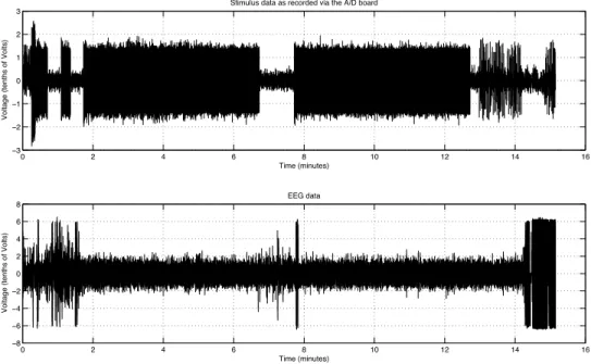
Figure 4.1. Data collected from an experimental session lasting about 15 minutes
(stimulus and EEG). The top graph shows stimulus data, as acquired by the A/D board. The
bottom graph shows EEG data. The signal is shown as-recorded, before the application of any signal pre-processing. The actual experiment begins slightly before the 2 minutes mark; by then, the subject was already wired but engaging in conversation until 30 seconds before the onset of the sounds belonging to the first experimental block. Around the 7-minute mark, there
was a minute of silence, separating the two experimental blocks. Data is from Subject 1.
Figure 4.2. Zoom to 3 seconds of data shown in figure 4.1. Data is shown as-recorded,
without the application of any signal pre-processing. The top and bottom graphs are synchronized. The top graph shows the acoustic stimuli as acquired by the A/D board, and the
bottom graph shows the EEG signal recorded from Fz. Data is from subject 1.
! " # $ % &! &" &# &$
!' !" !& ! & " ' ()*+,-*)./0+12 345067+,-0+.081,49,345012 :0)*/5/1,;606,61,<+=4<;+;,>)6,08+,?@A,B46<;
! " # $ % &! &" &# &$
!% !$ !# !" ! " # $ % ()*+,-*)./0+12 345067+,-0+.081,49,345012 CCD,;606
! "!! #!!! #"!! $!!! $"!! %!!!
!$ !#&" !# !!&" ! !&" # #&" $ '()*+,)-. /01234*+,2*526-+07+/012-. 82()919-+:323+3-+;*<0;:*:+=(3+26*+>?@+A03;:
! "!! #!!! #"!! $!!! $"!! %!!!
4.2.
SINGLE TRIALS4.2.1. EXAMPLES OF SINGLE TRIAL DATA
Examples of one hundred consecutive single trials, after filtering, baseline correction, and epoch
rejection, are shown in Figure 4.3. Trials are identified as standard or deviant.
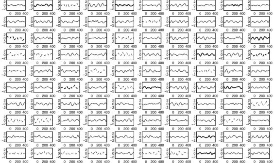
Figure 4.3. One-hundred consecutive single-trial recordings. Trials are sorted from top to
bottom and from left to right. Rejected trials are drawn in broken lines. Deviant epochs are drawn in double-weight lines. Data have been subject to filtering and baseline correction, as described in the previous chapter. Data are from the 100 first epochs of block 2 of Subject 1.
4.2.2. RESULTS OF DATA REJECTION PROCEDURES
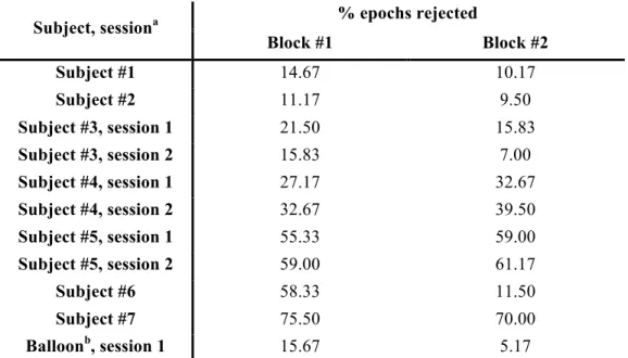
Data rejection is performed as described in the Experimentation chapter. The percentage of
rejected epochs in each block is indicated on Table 4.1. Data from subjects 5, 6, and 7 were
discarded, due to rejection of more than half the epochs. The number of remaining epochs of
each type, for each subject and session is shown in Table 4.2. These are the epochs that will be
used in the analysis that follows.
! "!! #!!
!" ! "
! "!! #!!
!" ! "
! "!! #!!
!" ! "
! "!! #!!
!" ! "
! "!! #!!
!" ! "
! "!! #!!
!" ! "
! "!! #!!
!" ! "
! "!! #!!
!" ! "
! "!! #!!
!" ! "
! "!! #!!
!" ! "
! "!! #!!
!" ! "
! "!! #!!
!" ! "
! "!! #!!
!" ! "
! "!! #!!
!" ! "
! "!! #!!
!" ! "
! "!! #!!
!" ! "
! "!! #!!
!" ! "
! "!! #!!
!" ! "
! "!! #!!
!" ! "
! "!! #!!
!" ! "
! "!! #!!
!" ! "
! "!! #!!
!" ! "
! "!! #!!
!" ! "
! "!! #!!
!" ! "
! "!! #!!
!" ! "
! "!! #!!
!" ! "
! "!! #!!
!" ! "
! "!! #!!
!" ! "
! "!! #!!
!" ! "
! "!! #!!
!" ! "
! "!! #!!
!" ! "
! "!! #!!
!" ! "
! "!! #!!
!" ! "
! "!! #!!
!" ! "
! "!! #!!
!" ! "
! "!! #!!
!" ! "
! "!! #!!
!" ! "
! "!! #!!
!" ! "
! "!! #!!
!" ! "
! "!! #!!
!" ! "
! "!! #!!
!" ! "
! "!! #!!
!" ! "
! "!! #!!
!" ! "
! "!! #!!
!" ! "
! "!! #!!
!" ! "
! "!! #!!
!" ! "
! "!! #!!
!" ! "
! "!! #!!
!" ! "
! "!! #!!
!" ! "
! "!! #!!
!" ! "
! "!! #!!
!" ! "
! "!! #!!
!" ! "
! "!! #!!
!" ! "
! "!! #!!
!" ! "
! "!! #!!
!" ! "
! "!! #!!
!" ! "
! "!! #!!
!" ! "
! "!! #!!
!" ! "
! "!! #!!
!" ! "
! "!! #!!
!" ! "
! "!! #!!
!" ! "
! "!! #!!
!" ! "
! "!! #!!
!" ! "
! "!! #!!
!" ! "
! "!! #!!
!" ! "
! "!! #!!
!" ! "
! "!! #!!
!" ! "
! "!! #!!
!" ! "
! "!! #!!
!" ! "
! "!! #!!
!" ! "
! "!! #!!
!" ! "
! "!! #!!
!" ! "
! "!! #!!
!" ! "
! "!! #!!
!" ! "
! "!! #!!
!" ! "
! "!! #!!
!" ! "
! "!! #!!
!" ! "
! "!! #!!
!" ! "
! "!! #!!
!" ! "
! "!! #!!
!" ! "
! "!! #!!
!" ! "
! "!! #!!
!" ! "
! "!! #!!
!" ! "
! "!! #!!
!" ! "
! "!! #!!
!" ! "
! "!! #!!
!" ! "
! "!! #!!
!" ! "
! "!! #!!
!" ! "
! "!! #!!
!" ! "
! "!! #!!
!" ! "
! "!! #!!
!" ! "
! "!! #!!
!" ! "
! "!! #!!
!" ! "
! "!! #!!
!" ! "
! "!! #!!
!" ! "
! "!! #!!
!" ! "
! "!! #!!
!" ! "
! "!! #!!
!" ! "
! "!! #!!
!" ! "
! "!! #!!
% epochs rejected Subject, sessiona
Block #1 Block #2
Subject #1 14.67 10.17
Subject #2 11.17 9.50
Subject #3, session 1 21.50 15.83
Subject #3, session 2 15.83 7.00
Subject #4, session 1 27.17 32.67
Subject #4, session 2 32.67 39.50
Subject #5, session 1 55.33 59.00
Subject #5, session 2 59.00 61.17
Subject #6 58.33 11.50
Subject #7 75.50 70.00
Balloonb, session 1 15.67 5.17
Table 4.1. Percentage of rejected epochs for each subject and session of experiments.
Epoch rejection is performed automatically as described in the Methods section. If more than
half the trials in a session are discarded, the data for the whole session is left out. As such, 3 subjects, namely, 5, 6, and 7, spanning 4 rounds, were eliminated from further analysis. a. For
subjects for which 2 sessions were run, the second block of the first round is the same as the first block of the second session, thus the equivalency in numerical values for percentage of rejected trials. b. All procedures for data collection and analysis were repeated on a balloon, to
validate the experimental setup against various possibilities for data contamination.
Subject, session SL DH SH DL
1 430 71 399 71
2 450 76 416 72
3,1 428 74 371 64
3,2 432 74 470 82
4,1 311 52 365 60
4,2 332 51 316 55
Table 4.2. Number of epochs of each type remaining after epoch rejection. SL: standard low
4.3.
A
NALYSIS OF EVOKED POTENTIALS4.3.1. AVERAGED WAVEFORMS
Plots of evoked potentials are shown in four figures. Figure 4.4 shows grand average curves for:
1. (tone, condition) pairs; 2. pMMN; 3. cMMN. Curves obtained in isolated rounds of
experiments, in an intra-subject basis, are shown in figures that follow it: 4.5, 4.6 and 4.7. Tables
of numerical values for peak amplitude and latency are provided for each of the figures.
Care should be exercised when looking at grand average curves (Figure 4.4), as there are
important inter-subject variations (Figures 4.5, 4.6, 4.7). Grand average plots were included
mostly so as to acknowledge the tradition in ERP research. One should look for possible
differences among the members of the ppMMN (the goal of this thesis) at both the individual and
the populational levels.
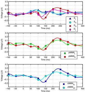
Figure 4.4. Grand-average waveforms. Tone onset is at the 0ms mark. Numbers for peak
amplitudes and latencies are shown in Table 4.3.
!!"" !#" " #" !"" !#" $"" $#" %"" %#" &""
!"'$ !"'! " "'! "'$ "'% ()*+,-*./ 012345+,-µ 0/ , , 6 7 6 8 9 8 9 7
!!"" !#" " #" !"" !#" $"" $#" %"" %#" &""
!"'$ !"'! " "'! "'$ "'% ()*+,-*./ 012345+,-µ 0/ , , :;;< 7 :;;< 8
!!"" !#" " #" !"" !#" $"" $#" %"" %#" &""
ERP Peak amplitude (µV) Peak latency (ms)
DH -0.165 136
DL -0.102 122
pMMNL -0.136 115
pMMNH -0.156 135
cMMNSL -0.182 136
cMMNSH -0.121 112
Table 4.3. Amplitude and latencies for grand average waveforms shown in Figure 5.4. No
peak in the MMN latency range can be identified for standard tones. pMMNL and cMMNSH are
calculated using DL and their latencies are in the [112, 115] ms interval; pMMNH, and cMMNSL are
calculated using DH, and their latencies are in the [135,136] ms interval.
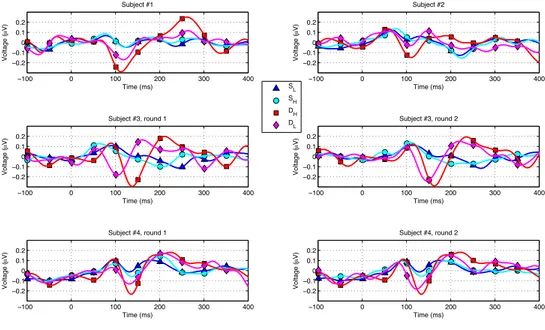
Figure 4.5. ERP’s for each (tone, condition). Potentials for each (tone, condition) are presented,
as average curves for each subject in each round of experiments. One round of experiments consists in the presentation of two blocks of stimuli, in which roles of tones as standard or deviant are reversed. The tones utilized are 196.0 and 466.2 Hz, each added of their first two harmonics. Rounds numbered “1” or left unmarked have the lower tone presented as standard in the first block; rounds numbered “2” have the higher tone presented as standard in the first block. Tone onset is at the 0ms mark. Probability of deviant is 15% regardless of which of the
two tones is used as deviant.
!!"" " !"" #"" $"" %""
!"&# !"&! " "&! "&# '()*+,)-. /01234*+, µ /. 5678*92+:! + + 5 ; 5 < =< =;
!!"" " !"" #"" $"" %""
!"&# !"&! " "&! "&# '()*+,)-. /01234*+, µ /. 5678*92+:#
!!"" " !"" #"" $"" %""
!"&# !"&! " "&! "&# '()*+,)-. /01234*+, µ /. 5678*92+:$>+?06@A+!
!!"" " !"" #"" $"" %""
!"&# !"&! " "&! "&# '()*+,)-. /01234*+, µ /. 5678*92+:$>+?06@A+#
!!"" " !"" #"" $"" %""
!"&# !"&! " "&! "&# '()*+,)-. /01234*+, µ /. 5678*92+:%>+?06@A+!
!!"" " !"" #"" $"" %""
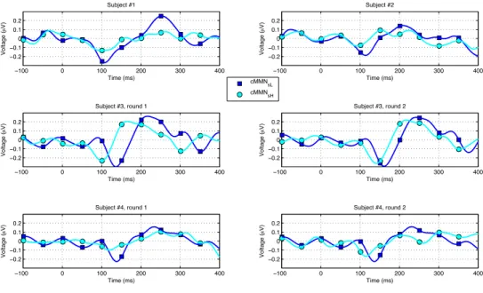
Figure 4.6. cMMN: cMMN plots are shown as subtraction of averaged curves, for each
subject and round of experiments. cMMN’s, or “classical” MMN’s, are computed as the
subtraction of the ERP for the standard from the ERP for the deviant. Standard and deviant stimuli are presented in random alternation, in the same block, and consist of physically different stimuli. This is how MMN is traditionally computed in the literature. The fact that the two curves presented in each graph are not the same is not enough to conclude that the MMN
is a distortion metric, as physical characteristics of the stimuli are different and other ERP components which may vary according to these characteristics could be lurking within the curves. Because of the presence of this sort of non-MMN ERP components in the MMN curve, it
is advisable to compute the MMN as what we call the “pure” MMN, shown in Figure 5.7. Tone onset is at the 0ms mark. Values for peak amplitudes and latencies are shown in Table 5.4.
Amplitude of cMMN peak
(µV) Latency of cMMN peak (ms) Subject,
round
cMMNsL cMMNsH cMMNsL cMMNsH
1, 1 -0.267 -0.133 108 99
2, 1 -0.187 -0.083 114 92
3, 1 -0.300 -0.233 136 100
3, 2 -0.294 -0.262 161 141
4, 1 -0.227 -0.100 138 119
4, 2 -0.227 -0.168 136 114
Table 4.4. Comparison of latencies and amplitudes of cMMNsL and cMMNsH peak amplitudes
and latencies, in the per-(subject, round) average waveforms.
!!"" " !"" #"" $"" %""
!"&# !"&! " "&! "&# '()*+,)-. /01234*+, µ /. 5678*92+:! + + 9;;< -= 9;;<->
!!"" " !"" #"" $"" %""
!"&# !"&! " "&! "&# '()*+,)-. /01234*+, µ /. 5678*92+:#
!!"" " !"" #"" $"" %""
!"&# !"&! " "&! "&# '()*+,)-. /01234*+, µ /. 5678*92+:$?+@06AB+!
!!"" " !"" #"" $"" %""
!"&# !"&! " "&! "&# '()*+,)-. /01234*+, µ /. 5678*92+:$?+@06AB+#
!!"" " !"" #"" $"" %""
!"&# !"&! " "&! "&# '()*+,)-. /01234*+, µ /. 5678*92+:%?+@06AB+!
!!"" " !"" #"" $"" %""
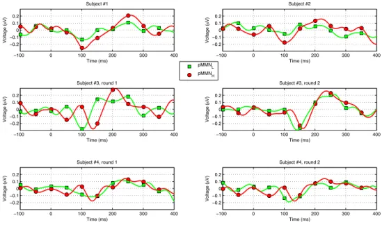
Figure 4.7. pMMN. pMMN’s are shown as subtraction of averaged curves, for each subject
and round of experiments. pMMN’s, or “pure” MMN’s, are computed as the subtraction of the
ERP for the standard from the ERP for the deviant, but, as opposed to how it’s traditionally done in the cMMN, standard and deviant consist of physically identical stimuli. This is achieved by
computing pMMN’s from two blocks of experiments, in which probability of deviant is kept constant, but roles of standard and deviant for each of the two different physical stimuli used
are exchanged. pMMN is the subtraction of the ERP for tone x presented as standard against tone y from the ERP of tone x presented as deviant against tone y. By doing this, the effects of non-MMN ERP components are completely cleared up, except of course for noise effects. If the cMMN were a distance metric, the curves for the two pMMN’s thus obtained would be the same;
according to the experimental results hereby shown this is not the case and the MMN is a distortion metric. Tone onset is at the 0ms mark. Values for peak amplitudes and latencies are
shown in Table 4.5.
Amplitude of pMMN peak
(µV) Latency of pMMN peak (ms) Subject,
round
pMMNL pMMNH pMMNL pMMNH
1, 1 -0.136 -0.262 108 107
2, 1 -0.067 -0.177 111 103
3, 1 -0.281 -0.280 102 137
3, 2 -0.294 -0.273 141 161
4, 1 -0.119 -0.177 130 134
4, 2 -0.190 -0.178 115 134
Table 4.5. Comparison of latencies and amplitudes of pMMN
L and pMMNH peak amplitudes
and latencies, in the per-(subject, round) average waveforms.
!!"" " !"" #"" $"" %""
!"&# !"&! " "&! "&# '()*+,)-. /01234*+, µ /. 5678*92+:! + + ;<<=> ;<<= ?
!!"" " !"" #"" $"" %""
!"&# !"&! " "&! "&# '()*+,)-. /01234*+, µ /. 5678*92+:#
!!"" " !"" #"" $"" %""
!"&# !"&! " "&! "&# '()*+,)-. /01234*+, µ /. 5678*92+:$@+A06BC+!
!!"" " !"" #"" $"" %""
!"&# !"&! " "&! "&# '()*+,)-. /01234*+, µ /. 5678*92+:$@+A06BC+#
!!"" " !"" #"" $"" %""
!"&# !"&! " "&! "&# '()*+,)-. /01234*+, µ /. 5678*92+:%@+A06BC+!
!!"" " !"" #"" $"" %""
4.3.2. MMN’S UNDER SAMPLE ANALYSIS
Statistical significance tests comparing epochs for standard and deviant, along with measures of
effect sizes, are given in Tables 4.6 and 4.7, for comparisons defined, respectively, by cMMN
(standard low x deviant high and standard high x deviant low) and pMMN (standard low x
deviant low and standard high x deviant high).
The statistical significance tests were run according to the methodology described in (Näätänen
et al., 2004), and, additionally, effect size measures were taken. Peak latency for every sample is
given by the peak latency in the average MMN curve calculated for each (subject, round). These
latency values are listed in tables 4.4 and 4.5, respectively, for cMMN and pMMN. Epoch
amplitude is given by the average amplitude in the 7 ms interval around the peak latency. Sample
peak amplitudes are compared by a paired t-test and by the effect size measure Cohen’s d, or d’,
which measures the difference between the sample means in units of pooled standard deviations,
as explained in the glossary (Cohen 1988).
SL x DH SH x DL
Subject,
round d’ P d’ p
1 0.43 0.0003 0.36 0.0041
2 0.28 0.0229 0.15 0.2268
3, 1 1.03 0.0000 0.54 0.0000
3, 2 0.40 0.0014 0.33 0.0056
4, 1 0.83 0.0000 0.33 0.0141
4, 2 0.83 0.0000 0.58 0.0001
Mean, standard deviation
(0.63, 0.3) (0.38,0.16)
Table 4.6. p-values and d’ for cMMN peak amplitudes. Amplitude was calculated as the
average amplitude in the 6ms interval centered around the peak of the cMMN average
waveform for each (subject, round). Sample analysis point to detection of significant (α = 3%)
cMMN for all Subjects and experimental blocks except for Subject number 2, blocks of type SH x
DL. A positive value for d’ indicates that the first term in the comparison has higher sample