www.atmos-chem-phys.net/16/2765/2016/ doi:10.5194/acp-16-2765-2016
© Author(s) 2016. CC Attribution 3.0 License.
On the characteristics of aerosol indirect effect based on dynamic
regimes in global climate models
Shipeng Zhang1,2,3, Minghuai Wang1,2,3, Steven J. Ghan3, Aijun Ding1,2, Hailong Wang3, Kai Zhang3, David Neubauer4, Ulrike Lohmann4, Sylvaine Ferrachat4, Toshihiko Takeamura5, Andrew Gettelman6, Hugh Morrison6, Yunha Lee7, Drew T. Shindell7, Daniel G. Partridge8,9,10, Philip Stier8, Zak Kipling8, and Congbin Fu1,2
1Institute for Climate and Global Change Research and School of Atmospheric Sciences, Nanjing University, Nanjing, China 2Collaborative Innovation Center of Climate Change, Jiangsu Province, China
3Atmospheric Science and Global Change Division, Pacific Northwest National Laboratory, Richland, Washington, USA 4ETH Zurich, Institute for Atmospheric and Climate Science, Zurich, Switzerland
5Research Institute for Applied Mechanic, Kyushu University, Fukuoka, Japan 6National Center for Atmospheric Research, Boulder, Colorado, USA
7Earth and Ocean Sciences, Nicholas School of the Environment, Duke University, Durham, North Carolina, USA 8Atmospheric, Oceanic and Planetary Physics, Department of Physics, University of Oxford, Oxford, UK
9Department of Environmental Science and Analytical Chemistry, Stockholm University, Stockholm, Sweden 10Bert Bolin Centre for Climate Research, Stockholm University, Stockholm, Sweden
Correspondence to:Minghuai Wang ([email protected])
Received: 5 August 2015 – Published in Atmos. Chem. Phys. Discuss.: 2 September 2015 Revised: 30 January 2016 – Accepted: 21 February 2016 – Published: 4 March 2016
Abstract.Aerosol–cloud interactions continue to constitute a major source of uncertainty for the estimate of climate ra-diative forcing. The variation of aerosol indirect effects (AIE) in climate models is investigated across different dynami-cal regimes, determined by monthly mean 500 hPa vertidynami-cal pressure velocity (ω500), lower-tropospheric stability (LTS)
and large-scale surface precipitation rate derived from sev-eral global climate models (GCMs), with a focus on liq-uid water path (LWP) response to cloud condensation nuclei (CCN) concentrations. The LWP sensitivity to aerosol per-turbation within dynamic regimes is found to exhibit a large spread among these GCMs. It is in regimes of strong large-scale ascent (ω500<−25 hPa day−1) and low clouds
(stra-tocumulus and trade wind cumulus) where the models differ most. Shortwave aerosol indirect forcing is also found to dif-fer significantly among difdif-ferent regimes. Shortwave aerosol indirect forcing in ascending regimes is close to that in sub-sidence regimes, which indicates that regimes with strong large-scale ascent are as important as stratocumulus regimes in studying AIE. It is further shown that shortwave aerosol indirect forcing over regions with high monthly large-scale
surface precipitation rate (>0.1 mm day−1) contributes the
most to the total aerosol indirect forcing (from 64 to nearly 100 %). Results show that the uncertainty in AIE is even larger within specific dynamical regimes compared to the un-certainty in its global mean values, pointing to the need to re-duce the uncertainty in AIE in different dynamical regimes.
1 Introduction
as rapid adjustments, known as the aerosol indirect effect(s) (AIE). These radiative effects are called Effective Radiative Forcing from aerosol–cloud interactions (ERFaci) (Boucher et al., 2013).
For liquid clouds, there are two principal ways through which aerosols interact with them in AIE. First, an increase in cloud condensation nuclei (CCN) concentration from an-thropogenic aerosols leads to smaller cloud droplet sizes as-suming constant liquid water content. The increased num-ber but decreased droplet sizes in turn increase cloud albedo due to more efficient backscattering. This is called the cloud albedo effect or the first AIE, also known as the Twomey effect (Twomey, 1977). Moreover, the smaller cloud droplet sizes are hypothesized to lead to decreases in precipitation efficiency, which may further alter cloud liquid water path (LWP) and cloud lifetime (Albrecht, 1989). These adjust-ments are also referred to as the cloud lifetime effect or the second AIE. It is worth noting that delaying the onset of pre-cipitation may further modify latent heating profiles, which could lead to the invigoration of convective clouds (e.g., An-dreae et al., 2004; Rosenfeld et al., 2008). There are also adjustments on mixed-phase and ice clouds (e.g., Storelvmo et al., 2008; Lohmann and Hoose, 2009; Liu et al., 2012b; Wang et al., 2014). The focus of this study is on liquid cloud response to aerosol perturbation, primarily from large-scale clouds.
AIE could be large enough to offset much of the global warming induced by anthropogenic greenhouse gases, yet its magnitude is still very uncertain (IPCC, 2013). The uncer-tainty in the cloud lifetime effect of aerosols is particularly large.
The complexity of microphysical-dynamical-radiative feedbacks involved in the cloud lifetime effect has been noted in previous studies. Conventional theory regarding the cloud lifetime effect suggests that higher CCN concentration slows down precipitation formation and hence leads to more LWP (Albrecht, 1989). However, this theory is inconsistent with some observations (Coakley and Walsh, 2002; Kaufman et al., 2005; Matsui et al., 2006; Chen et al., 2014) and large eddy simulations (LESs) (e.g., Ackerman et al., 2004; Lu and Seinfeld, 2005; Wang and Feingold, 2009b) that found either an increase or decrease in LWP in responses to increases in CCN concentration.
Further modeling studies (e.g., Ackerman et al., 2004; Stevens and Feingold, 2009; Guo et al., 2011) suggest that cloud top entrainment plays a critical role as a dynamic feed-back, to balance LWP and modify the lifetime of bound-ary layer clouds. Ackerman et al. (2004) found that an in-crease in droplet number concentration (Nd)reduces cloud
water sedimentation while accelerating the cloud-top entrain-ment rate, which makes the humidity of air overlying the boundary layer, wet or dry, critically important in deter-mining the response of LWP. When surface precipitation is weak (<0.1 mm day−1)and the overlying air is dry, LWP
decreases in response to increasing aerosol. They showed
that the entrainment rate was reduced by decreasing avail-able boundary-layer turbulence kinetic energy (TKE). How-ever, Bretherton et al. (2007) found that TKE remained un-changed and changes in entrainment rate are mainly caused by reduced evaporative cooling from removing out liquid wa-ter. LES studies (e.g., Wang and Feingold, 2009a) with a large model domain that is able to resolve mesoscale circu-lations (on the order of ten kilometers) in marine stratocu-mulus showed that aerosols can shift cloud regimes through their impact on precipitation and associated dynamical feed-backs. This can represent a more significant impact on cloud radiative forcing than the conventional AIE.
Many state-of-the-art global climate models (GCMs) ap-pear to overestimate AIE when compared with satellite ob-servations (e.g., Quaas et al., 2009; Wang et al., 2012), de-spite some uncertainties in satellite-derived estimates (e.g., Penner et al., 2011; Gryspeerdt et al., 2014a, b). The multi-scale interactions between clouds, aerosols, and large-multi-scale dynamics (Stevens and Feingold, 2009; Wang et al., 2011; Ma et al., 2015) and complex microphysical processes (e.g., Bretherton et al., 2007; Gettelman et al., 2013) cause uncer-tainties in estimating AIE by GCMs. One possible source of overestimation of AIE is their inability to reproduce nega-tive LWP responses to aerosol perturbations, which are found in some observations and LES studies, partly because they do not explicitly simulate the droplet size effect on the en-trainment process and on sub-grid cloud organizations asso-ciated with changes in precipitation. Guo et al. (2011) found that this effect could be captured through applying a param-eterization based on multi-variate probability density func-tions with dynamics (MVD PDFs) in single-column simula-tions. They found decreased LWP in response to increasing aerosols concentration and suggested that the implementa-tion of MVD PDFs in GCMs may help lower the magni-tude of the simulated AIE. A negative correlation between LWP and aerosol loading was further found for clouds with weak precipitation and dry air above the PBL in a subsequent global model study (Guo et al., 2015).
Another likely source for the overestimation of cloud life-time effects in GCMs is the treatment of cloud microphysics (Penner et al., 2006; Posselt and Lohmann, 2009; Wang et al., 2012). In warm clouds, cloud microphysical processes are dominated by autoconversion and accretion in bulk mi-crophysics schemes (Gettelman et al., 2013). Since autocon-version acts as a sink of LWP, it is crucial in the formation of precipitation, and thus plays an important role in determining the cloud lifetime effect. The autoconversion rate is directly dependent on droplet number concentration (Nd)while the
accretion rate is only weakly dependent onNd
in GCMs. They showed that the adoption of different rain schemes (prognostic vs. diagnostic) in a GCM leads to a dif-ferent LWP response to aerosol perturbations. A prognostic rain scheme can shift the importance of (warm) rain pro-duction from autoconversion process to the accretion process and therefore reduces the AIE (Posselt and Lohmann, 2009; Gettelman et al., 2015). However, Hill et al. (2015) shows that adding prognostic rain scheme alone still cannot reduce the spread of susceptibility of precipitation among differ-ent cloud microphysics parameterizations and further shows that increasing the complexity of the rain representation to double-moment significantly reduces the spread of precipi-tation sensitivity and improves overall consistency between bulk and bin schemes.
Previous studies are mostly confined to global averages (e.g Quaas et al., 2009; Wang et al., 2012) or a specific dynamic environment (e.g., Bretherton et al., 2007; Guo et al., 2011). However, aerosols, clouds, precipitation distribu-tions, and dynamical feedbacks are all related to the pre-vailing meteorological environment (Stevens and Feingold, 2009). Clouds are sensitive to changes in dynamical regimes, which can be defined by large-scale circulations, thermody-namic structure, and meteorological backgrounds (Bony et al., 2004). Gryspeerdt and Stier (2012) and Gryspeerdt et al. (2014c) used satellite data and found that the characteris-tics of aerosol cloud-albedo effect (droplet number sensitiv-ity) vary with cloud regimes and pointed out the importance of regime-based studies of aerosol–cloud interactions.
In this study, we investigate how AIE in several GCMs varies under different dynamical regimes over global oceans (60◦S–60◦N), with a focus on cloud lifetime effects of
aerosols (2nd AIE). We note that the term “cloud lifetime effects” can be somehow misleading, since aerosol effects on cloud liquid water may have little to do with cloud life-time per se (e.g., Small et al., 2009). Nevertheless, this term is still used in some occasions in this paper for convenience. The paper is organized as follows. Methods and models are described in Sect. 2, and results and discussions are presented in Sect. 3. The paper concludes with the summary in Sect. 4.
2 Methodology and models
The response of LWP to aerosol perturbations is defined as
λ=d ln LWP/d ln CCN. (1)
As simulated LWP and CCN can be quite differ-ent among GCMs, the logarithmic form of LWP and CCN is adopted in the λ formula. λ is a metric to quantitatively measure cloud lifetime effect of aerosols in models. It is directly calculated as the relative change of monthly mean LWP from pre-industrial (PI) to present day (PD) divided by the relative change of CCN. Here d ln LWP=(LWPPD−LWPPI)/LWPPI and
d ln CCN=(CCNPD−CCNPI)/CCNPI, where LWPPD and
LWPPI are LWP in PD and PI, respectively, while CCNPD
and CCNPIare CCN in PD and PI, respectively. This
param-eter was used by Wang et al. (2012) to constrain the cloud lifetime effects of aerosols over global oceans using precip-itation frequency susceptibility (Spop)derived from A-Train
satellite observations. Lebo and Feingold (2014) examined the relationship betweenλandSpopto aerosol perturbations
for stratocumulus and trade-wind cumulus simulated by LES and found thatλmay increase in marine stratocumulus while decrease in the case of trade-wind cumulus in response to in-creasingSpop, suggesting a cloud regime dependence of this
relationship. Note thatλallows some feedbacks, for example cloud effects on CCN.
Dynamical regimes can be defined by environment char-acteristics such as large-scale vertical pressure velocity (e.g., Bony and Dufresne, 2005) and lower-tropospheric stabil-ity (LTS, defined as the difference in potential tempera-ture between 700 hPa and the surface,θ700hPa–θsurface)(e.g.,
Medeiros and Stevens, 2011). Medeiros and Stevens (2011) noted that low clouds and deep convective clouds could be separated by ω500 while different low cloud types under
large-scale subsidence can only be depicted by using LTS. In this study the monthly averaged vertical pressure velocity (ω)in the mid-troposphere (defined as at 500 hPa) is used as a proxy for large-scale motions (Bony and Dufresne, 2005). Note that ω500 with positive (negative) value means
de-scending (ade-scending) motions. We decompose global (60◦S–
60◦N) large-scale circulations over ocean as a group of
dy-namical regimes (equally sampled) byω500(and LTS).
As-cending regimes and desAs-cending regimes are defined byω500
and descending regimes are further divided into stratocumu-lus, transitional clouds and trade wind cumulus regimes by LTS. This method is straight-forward to apply to GCM re-sults and gives us a direct view of the relationship between clouds and their favorable large-scale environmental charac-teristics. Note however that the use of monthly means may obscure some details in the microphysical relationships, es-pecially where the variability of cloud properties is high.
Since vertical pressure velocity is used as a major crite-rion here, dynamic regimes generally follow the features of vertical pressure velocity distributions. Descending regimes are mostly located at subtropical regions and western coasts of continents, while ascending regimes locates around the Inter-tropical Convergence Zone (ITCZ) and northern Pa-cific where storm tracks prevail. The seasonal evolution of dynamic regimes follows seasonal changes in the major me-teorological systems. For example, ascending regimes move north and/or south as ITCZ move north and/or south and de-scending regimes move accompanying with subtropical high move. The characteristics of dynamic and thermodynamic regimes were discussed in detail in Bony et al. (2004).
As the perturbations in cloud radiative forcing from an-thropogenic aerosols (indirect effect) are typically on the or-der of 1 W m−2, which is small compared to the cloud
Table 1.The types of clouds included in liquid water path (LWP) and surface rain rate and different rain schemes in 10 participating models
Model LWP Rain Rain scheme
CAM5 Sa S dc
CAM5-MG2 S S pd
CAM5-PNNL S S d
CAM5-CLUBB S+shallow convective clouds S+shallow convective clouds d CAM5-CLUBB-MG2 S+shallow convective clouds S+shallow convective clouds p ECHAM6-HAM2 S+convective detrainment S d
SPRINTARS S+Cb S+C d
SPRINTATRS-KK S+C S+C d
ModelE2-TOMAS S+anvil clouds S+anvil clouds d
HadGEM3-UKCA S+C S p
aS in LWP and Rain stands for stratiform clouds.bC in LWP and Rain stands for convective clouds.cd in Rain schemes represents
diagnostic rain scheme.dp in Rain schemes represents prognostic rain scheme.
and longwave radiative effect of ∼27 W m−2)(Boucher et
al., 2013), long integrations are required to produce statis-tically significant results. The Newtonian relaxation method (nudging) provides a way to estimate AIE within a relatively short integration time, while giving statistically significant results (Lohmann and Hoose, 2009; Kooperman et al., 2012). Nudging here refers to the method of adding a forcing to the prognostic model equations, determined by the difference be-tween a model-computed value and a prescribed value at the same time and model grid-cell, to constrain the model re-sults with prescribed atmospheric conditions. Kooperman et al. (2012) implemented nudging to constrain PD and PI sim-ulations toward identical meteorological fields and found that the use of nudging provided a more stable estimate of AIE in shorter simulations and increased the statistical significance of the anthropogenic aerosol perturbation signal. All simula-tions used in this study were nudged toward reanalysis winds (year 2006 to 2010) provided by operational forecast cen-ters. Some simulations were further nudged toward reanal-ysis temperature, but this was discouraged because it might affect the moist convection activities simulated in the model (Zhang et al., 2014). All models were driven by the same IPCC aerosol emissions for years 1850 and 2000 (Lamarque et al., 2010) and 5-year simulations were performed in each case (PI and PD). Sea surface temperature, sea-ice extent and greenhouse gas concentrations are prescribed to climatolog-ical values in all simulations. Monthly data were then ob-tained by averaging over the 5-year integration period.
Onlyω500in PD runs is used to derive dynamical regimes
and then these dynamical regimes are applied to PI simula-tions as well, with the assumption thatω500does not change
much from PI to PD. This assumption is reasonable as both PD and PI runs were nudged toward the reanalysis data here, which ensuresω500is very similar between PD and PI.
A total of 10 aerosol-climate models participated in this study. This includes five versions of Community Atmosphere Model (CAM) 5.3, and two versions of SPRINTARS. These models show large differences in
their aerosol and cloud treatments. For example, while most models (CAM5, PNNL, MG2, CAM5-CLUBB, CAM5-CLUBB-MG2, ECHAM6-HAM2, and SPRINTARS-KK) use the autoconversion scheme from Khairoutdinov and Kogan (2000, hereafter KK), autocon-version rate in ModelE-TOMAS is independent of cloud droplet number concentration and the Berry scheme (Berry, 1968) is used for SPRINTARS. Most models use diagnos-tic rain schemes, while an updated Morrison and Gettel-man (2008) microphysics scheme with a prognostic rain scheme (MG2) (Gettelman et al., 2015) is adopted in CAM5-MG2 and CAM5-MG2-CLUBB. HadGEM3-UKCA also adopts a prognostic rain scheme (Abel and Boutle, 2012). While most models only account for aerosol ef-fects on large-scale stratiform clouds, CAM5-CLUBB and CAM5-CLUBB-MG2 use a higher-order turbulence closure (CLUBB) to unify the treatment of boundary layer turbu-lence, stratiform clouds, and shallow convection, and there-fore include aerosol effects on shallow convection (Bogen-schutz et al., 2013). A brief description of each model is pro-vided in Appendix A.
3 Results
3.1 Annual mean
We first examine the annual climatology in different simu-lations to get an overall picture of the general differences and/or similarities among these models (details within dy-namic regimes are examined in Sect. 3.2). All of the simula-tions reproduce the general pattern of large-scale circulasimula-tions (ω500): strong ascending motions within the inter-tropical
convergence zone (ITCZ) and subsidence dominating sub-tropical eastern ocean regions (not shown). The similar pat-terns ofω500 (due to nudging) in these simulations ensure
that dynamic regimes defined byω500do not vary much
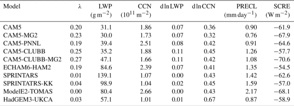
Table 2.Global ocean (60◦S–60◦N) averages of LWP, column-integrated cloud condensation nuclei (CCN, at 0.1 % supersaturation)
con-centration, precipitation rate (PRECL), shortwave cloud radiative effect (SCRE) derived from the present-day (PD) cases and the relative change from pre-industrial (PI) to PD of LWP and CCN (d ln LWP and d ln CCN) and the sensitivity of LWP to CCN concentration change (λ, d ln LWP/d ln CCN) of the 10 GCM simulations.
Model λ LWP CCN d ln LWP d ln CCN PRECL SCRE (g m−2) (1011m−2) (mm day−1) (W m−2)
CAM5 0.20 31.1 1.86 0.07 0.36 0.90 −61.9 CAM5-MG2 0.23 30.0 1.73 0.07 0.32 0.76 −67.9 CAM5-PNNL 0.19 39.4 2.51 0.08 0.42 0.91 −64.6 CAM5-CLUBB 0.25 35.2 1.88 0.11 0.45 1.26 −57.7
CAM5-CLUBB-MG2 0.27 47.1 1.66 0.11 0.42 1.08 −70.6 ECHAM6-HAM2 0.19 84.6 2.39 0.07 0.41 1.35 −54.5 SPRINTARS 0.01 139.1 1.07 0.00 0.43 1.42 −62.6 SPRINTATRS-KK 0.04 98.9 1.04 0.02 0.45 1.59 −57.0 ModelE2-TOMAS 0.00 80.4 2.66 0.00 0.43 2.17 −68.1 HadGEM3-UKCA 0.03 57.1 1.01 0.01 0.67 0.87 −58.9
Table 1 lists the types of clouds included in LWP and rain analyzed in this study and the different rain scheme (prognostic or diagnostic) in these 10 GCM simulations. Ta-ble 2 lists global annual means of aerosol, precipitation and cloud parameters in PD simulations and λfor each model. Note that all versions of CAM5 calculate LWP only for large-scale clouds while SPRINTARS, SPRINTARS-KK and HadGEM3-UKCA also count LWP from convective clouds. As for ModelE2-TOMAS, LWP includes stratiform anvil clouds that formed from convective detrainment of water va-por and ice. ECHAM6-HAM2 also includes the contribution of convective detrainment of liquid water and ice to strati-form clouds. Also note that CAM5 models with CLUBB in-clude LWP in the shallow convective regimes, which partly explains why these models produce more LWP than their cor-responding CAM5 models without CLUBB (Table 2).
There are large differences among global LWP annual means. CAM5-MG2 has the lowest LWP among these sim-ulations (30.0 g m−2). The LWP means over oceans are
31.1, 39.4, and 35.2 g m−2 in CAM5, CAM5-PNNL, and
CAM5-CLUBB, respectively. HadGEM3-UKCA simulates higher LWP (57.1 g m−2)than all versions of CAM5. LWPs
in ModelE2-TOMAS (80.4 g m−2) and ECHAM6-HAM2
(84.6 g m−2)are greater than the aforementioned GCMs, but
less than in SPRINTARS and SPRINTARS-KK (139.1 and 98.9 g m−2respectively) which include LWP from
convec-tive clouds. Even though CAM5-CLUBB simulates a higher LWP in storm track regions and ECHAM6-HAM2 produces much more LWP associated with deep convection in the ITCZ, all models here display reasonable patterns of global LWP distributions (not shown).
The differences in CCN (at 0.1 % supersaturation) among these simulations are not as large as the differences in LWP (Table 2). The global annual mean CCN in CAM5-PNNL, which has a different treatment of wet scavenging processes (Wang et al., 2013), is slightly larger than the
one in other versions of CAM5. CCN concentrations sim-ulated by CAM5-PNNL, ECHAM6-HAM2, and ModelE2-TOMAS are largest among these simulations and are more than twice those simulated by SPRINTARS, SPRINTARS-KK and HadGEM3-UKCA, which are the lowest. Since these models are using the same emissions, differences of CCN between the models are mainly due to different aerosol lifetime between models.
The LWP response to aerosol perturbations, λ, in ECHAM6-HAM2 (0.19) is close to those derived from three CAM5 configurations (0.20 in CAM5, 0.19 in CAM5-PNNL and 0.25 in CAM5-CLUBB). Notice thatλin CAM5-MG2 and CAM5-CLUBB-CAM5-MG2 is larger than that in CAM5 and CAM5-CLUBB, respectively, which indicates that the changes of LWP in the models, using the MG2 scheme, are more sensitive to the aerosol perturbations. LWP is much less sensitive to the changes of CCN in SPRINTARS and SPRINTARS-KK withλof 0.01 and 0.04 respectively.λis also small in HadGEM3-UKCA (0.03) due to the large rel-ative increase of CCN and a small relrel-ative increase of LWP. Since the aerosol effect on precipitation formation is turned off in ModelE2-TOMAS (its autoconversion parameteriza-tion is not a funcparameteriza-tion ofNd), LWP barely responds to the
increase of CCN (λis−0.001). The variation inλclosely fol-lows that of the relative enhancement of LWP (d ln LWP), as the variation of the relative enhancement of CCN (d ln CCN) among the simulations is generally much smaller than that of d ln LWP.
We should note that large differences in CCN shown in Table 2 do not necessarily correspond to equally large dif-ferences in droplet concentration (Nd), sinceNdis primarily
−50 0 50 0 50 100 150 200
ω500 (hPa/d)
LWP (g/m2)
(a)
−50 0 50
0 1 2 3
x 1011
ω500 (hPa/d) (b) CCN (#/m2) CAM5 CAM5−MG2 CAM5−PNNL CAM5−CLUBB CAM5−CLUBB−MG2 ECHAM6−HAM2 SPRINTARS SPRINTARS−KK ModelE2−TOMAS HadGEM3−UKCA
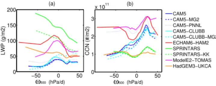
Figure 1. (a)LWP and(b)column-integrated CCN (at 0.1 % super-saturation) as a function of 500 hPa vertical pressure velocity (ω500)
derived from different models: CAM5 (blue solid line), MG2 (blue dashed line), PNNL (blue dotted line), CAM5-CLUBB (cyan solid line), CAM5-CAM5-CLUBB-MG2 (cyan dashed line), ECHAM6-HAM2 (red solid line), SPRINTARS (green solid line), SPRINTARS-KK (green dashed line), ModelE2-TOMAS (purple solid line) and HadGEM3-UKCA (orange solid line).
into how clouds’ response toNdchanges since LWP directly
depends onNd, not necessarily on CCN. However, this
alter-native definition ofλas d ln LWP/d lnNdwould be difficult
to compare with observations, and this also does not directly measure cloud response to anthropogenic aerosols. The in-teractions between clouds and anthropogenic aerosols arise through a chain of processes, from effects of the CCN on
Ndto effects ofNdon cloud water, which can be expressed as
d ln LWP/d ln CCN=(d ln LWP/d lnNd)·(d lnNd/d ln CCN).
This chain of processes has now been examined in Ghan et al. (2016) based on the same set of model simulations documented in this study.
3.2 Regime dependence 3.2.1 LWP, CCN, andλ
Figure 1 shows LWP and CCN as a function of vertical pres-sure velocity at 500 hPa (ω500)derived from PD simulations.
To derive Fig. 1, the 12-month monthly global grid values are first sorted into 20 dynamical regimes according to their
ω500 values, keeping the number of samples in each bin equal. LWP, CCN, and values of other fields for each bin are then calculated from averaging the values of all samples in that particular bin.
In general, SPRINTARS (default and KK) simulates much higher LWP in all dynamic regimes and ECHAM6-HAM2/ModelE2-TOMAS in most regimes than different versions of CAM5 runs (default, PNNL, CLUBB and MG2) (Fig. 1a), which is consistent with global means in Ta-ble 2. A peak of LWP is found around ω500=0 hPa day−1 in CAM5, ModelE2-TOMAS, and ECHAM6-HAM2. For SPRINTARS, LWP decreases from 190 to 100 g m−2asω
500
increases from−60 to 40 hPa day−1. In all simulations LWP
is low in regimes where ω500 is larger than 10 hPa day−1,
i.e., regimes dominated by low clouds. HadGEM3-UKCA simulates larger LWP than CAM5 especially in ascending
−50 0 50
0 0.2 0.4
ω500 (hPa/d)
dlnLWP/dlnCCN
(a)
−50 0 50
0 0.1 0.2
ω500 (hPa/d)
dlnLWP
(b)
−50 0 50
0 0.2 0.4 0.6
ω500 (hPa/d)
dlnCCN (c) CAM5 CAM5−MG2 CAM5−PNNL CAM5−CLUBB CAM5−CLUBB−MG2 ECHAM6−HAM2 SPRINTARS SPRINTARS−KK ModelE2−TOMAS HadGEM3−UKCA
Figure 2.Same as Fig. 1a, but for(a)the sensitivity of LWP to the change of CCN (λ),(b) relative enhancement of liquid water path (d ln LWP) and(c)relative enhancement of cloud condensation nuclei (d ln CCN) from pre-industrial (PI) to present day (PD).
regimes. The model spread of LWP response is larger in the ascending regimes than in the subsiding regimes. This may be partly related to the fact that the types of clouds included in LWP are not the same in different models (Ta-ble 1). Figure 1b shows that CCN concentrations peak at around 25 hPa day−1 among all the models. This peak is
partly caused by little precipitation (and therefore low wet scavenging rate) in subsidence regimes as well as by the fact that these dynamic regimes are located near continents where the sources of anthropogenic aerosols are strong. Further-more, CCN concentrations are low at around 0 hPa day−1,
which could be explained by the fact that most regimes around 0 hPa day−1 are located over the oceans far away
from continents (i.e. remote marine aerosols) and anthro-pogenic aerosol source regions (figures not shown). Gener-ally, CCN in two versions of SPRINTARS and HadGEM3-UKCA is less than other models in most regimes, consistent with Table 2.
We note that although the global means ofλin all CAM5 configurations and ECHAM6-HAM2 are close, from 0.19 in ECHAM6-HAM2 to 0.25 in CAM5-CLUBB, λ in the different dynamical regimes can differ significantly among these simulations (Fig. 2). For example, LWP in CAM5-PNNL is much more sensitive to CCN perturbations than in ECHAM6-HAM2 in strong ascending regimes; and in strong subsidence regimes, LWP in CAM5-CLUBB and ECHAM6-HAM2 is more sensitive than in CAM5-PNNL and CAM5. Models that use the MG2 with prognostic rain scheme (i.e. CAM5-MG2 and CAM5-CLUBB-MG2) simulate larger λ
than the models that use the default MG scheme in most regimes, only except for strong subsidence regimes. How-ever, generally the shapes of theλdistribution are very sim-ilar. λ in CAM5-CLUBB-MG2 is large in both ascending and subsidence regimes, which explains the largest global
λ in CAM5-CLUBB-MG2 among all configurations (Ta-ble 2). Except for the models producing very low values of λ (SPRINTARS, SPRINTARS-KK, ModelE2-TOMAS and HadGEM3-UKCA),λfrom the other models converges around 0 hPa day−1 and then diverges greatly in strong
as-cending regimes (from 0.10 to 0.46) and, to a lesser extent, in strong subsidence regimes. This indicates that it is in regimes with weak vertical velocity where models agree most, while it is in strong ascending and descending regimes where mod-els differ most. The diversity ofλwithin dynamical regimes in different GCMs highlights the need to distinguish different dynamical regimes in studying AIE.
When analyzing the numerator and denominator ofλ sep-arately, we found that this large spread in λis mainly con-tributed by the numerator, d ln LWP. d ln LWP ranges from about 0 to 0.22 among the models (Fig. 2b), while the de-nominator d ln CCN is more stable than d ln LWP within dy-namical regimes and fluctuates around 0.45, except for larger d ln CCN in HadGEM3-UKCA (Fig. 2c). In summary, the ra-tio of d ln LWP to d ln CCN (λ)therefore changes more con-sistently with d ln LWP within dynamical regimes.
The decreasing trends of λwith increasingω in CAM5, CAM5-MG2, and CAM5-PNNL are similar, which is oppo-site to the increasing trends derived from ECHAM6-HAM2, CAM5-CLUBB, and CAM5-CLUBB-MG2. It is interest-ing that the regime-dependence of λ simulated by CAM5-CLUBB and CAM5-CAM5-CLUBB-MG2 is quite different from that simulated by CAM5, CAM5-MG2, and CAM5-PNNL even though all these five model versions are originally from CAM5 and share many similarities. In CAM5, CAM5-MG2, and CAM5-PNNL, three separate parameterization schemes are used to treat planetary boundary layer (PBL) turbu-lence, stratiform cloud macrophysics, and shallow convec-tion. In CAM5-CLUBB and CAM5-CLUBB-MG2, instead, a higher-order turbulence closure, Cloud Layers Unified by Binormals (CLUBB), is adopted to replace these three sepa-rate schemes to provide a unified treatment of these processes (Bogenschutz et al., 2013). A major improvement of CAM-CLUBB is the better simulation of the transition of
stratocu-mulus to trade wind custratocu-mulus over subtropical oceans (Bo-genschutz et al., 2013). Figure 2a shows thatλin CAM5-CLUBB and CAM5-CAM5-CLUBB-MG2 is quite different from that in CAM5 simulations without CLUBB (i.e., CAM5, CAM5-MG2 and CAM5-PNNL) in regimes whereω500 is
larger than 10 hPa day−1. Under such suppressed conditions,
low clouds such as trade wind cumulus and stratocumulus are typically formed. This higherλmight be expected because CAM5-CLUBB formulations apply the MG microphysics (and effects of aerosols on cloud microphysics) to shallow convective regimes. The better representation of low clouds in CAM5-CLUBB, and the representation of double-moment microphysics and AIE in shallow convective regimes from the unified parameterization may help to explain the differ-ent behaviors between CAM5 runs with CLUBB (CAM5-CLUBB and CAM5-(CAM5-CLUBB-MG2) and CAM5 runs without CLUBB (CAM5, CAM5-MG2 and CAM5-PNNL) in subsi-dence regimes.
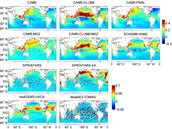
In order to find out the crucial geographic locations of dynamic regimes where d ln LWP differs most in Fig. 2b, we plot the global distribution of annual averaged d ln LWP in different simulations, shown in Fig. 3. The ascending regimes where ECHAM6-HAM2 differs significantly from the two CAM5 configurations (CAM5, CAM5-PNNL) are located over the North Pacific Ocean (from 30 to 60◦N),
for weak ascending motions and the southern coast of Asia for strong ascending motions. The spatial patterns in ECHAM6-HAM2, CAM5-CLUBB, CAM5-CLUBB-MG2, and HadGEM3-UKCA share some similarities over the northern Pacific Ocean, but the magnitude in CAM5-CLUBB and CAM5-CLUBB-MG2 is larger than in ECHAM6-HAM2 and HadGEM3-UKCA. Moreover, not only the spa-tial pattern but also the magnitude of d ln LWP in ECHAM6-HAM2 differ significantly from those in CAM5, CAM5-MG2 and CAM5-PNNL. For the southern coast of Asia where strong ascending motions dominate, all simulations show a relative increase of LWP. However, d ln LWP in ECHAM6-HAM2 in this region is much smaller than in all CAM5 simulations. This makes d ln LWP, and thus λ, in ECHAM6-HAM2 much less than in the five CAM5 mod-els (CAM5, CAM5-MG2, CAM5-PNNL, CAM5-CLUBB, and CAM5-CLUBB-MG2) in ascending regimes, as shown in Fig. 2b and a.
Figure 3.Relative change of annual averaged LWP from PI to PD (d ln LWP) simulations derived from the 10 GCM simulations.
global ocean. SPRINTARS-KK simulates the same pattern as SPRINTARS only with larger values. Meanwhile, d ln LWP in ModelE2-TOMAS shows no special global pattern and the values are all near zero, which indicates LWP in ModelE2-TOMAS has indeed little response to aerosol perturbations as autoconversion rate in ModelE2-TOMAS is not influenced by cloud droplet number concentrations.
Figure 3 shows that the differences in subsidence regimes in Fig. 2b are mainly contributed by middle northern sub-tropical oceans and western coasts of continents. In middle northern subtropical oceans, the relative changes of LWP in ECHAM6-HAM2, HadGEM3-UKCA and the two CAM5 models with CLUBB (CAM5-CLUBB and CAM5-CLUBB-MG2) are much more sensitive to the aerosol perturbations than in the three CAM5 models without CLUBB (CAM5, CAM5-PNNL, and CAM5-MG2), even though d ln LWP in ECHAM6-HAM2 and HadGEM3-UKCA is not as large as that in CAM5-CLUBB and CAM5-CLUBB-MG2. An-other difference among these models is in regions dominated by more intensive subsidence, over the western coasts of North America, South America, and Africa. In these regions d ln LWP in ECHAM6-HAM2 and the two CAM5 models with CLUBB is large while it is small in the three CAM5 models without CLUBB.
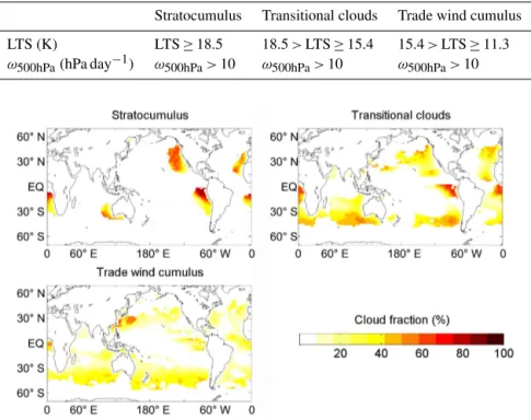
To examine the cloud lifetime effect in different cloud regimes more specifically, another criterion, lower-tropospheric stability (LTS=θ700hPa-θsurface), is added to
distinguish stratocumulus from trade wind cumulus regimes,
following Medeiros and Stevens (2011). Table 3 lists the cri-teria of different low cloud types conditionally sampled by
ω500and LTS. The annual mean cloud fractions of each low
cloud type in CAM5-CLUBB are shown in Fig. 4; the distri-butions in other simulations are generally similar to CAM5-CLUBB (figures not shown). The cloud type distribution is consistent with satellite observations which show that stra-tocumuli occur over subtropical oceans near western conti-nents while trade wind cumuli dominate over oceans further away from continents (Medeiros and Stevens, 2011). Fig-ure 4 shows that some differences in d ln LWP between mod-els shown in Fig. 3 are located at regions dominated by low clouds (i.e., stratocumulus and trade wind cumulus).
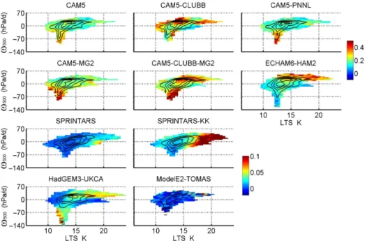
The joint distributions of LTS andω500over global oceans between 60◦S and 60◦N derived from the models are shown
in Fig. 5. Note that the bins here are not equally sampled as in previous figures but divided into equal LTS andω inter-vals. LTS ranges from 8 to 24 K whileωranges from−100 to 60 hPa day−1. Instances with slight downward vertical
mo-tions and moderate LTS are most frequent.
Figure 5 shows that, thoughω500 plays the primary role
Table 3.Criteria used to conditional sampling stratocumulus, transitional clouds, and trade wind cumulus regimes (adopted from Medeiros and Stevens, 2011).
Stratocumulus Transitional clouds Trade wind cumulus LTS (K) LTS≥18.5 18.5>LTS≥15.4 15.4>LTS≥11.3
ω500hPa(hPa day−1) ω
500hPa>10 ω500hPa>10 ω500hPa>10
Figure 4.The annual mean cloud fraction (averaged on the months when the regime occurs) of stratocumulus regime (top left), transi-tional clouds regime (top right) and trade wind cumulus regime (bottom left) derived from PD monthly simulation in CAM5-CLUBB. The definitions of different cloud types are listed in Table 3.
in ascending regimes is larger than in regimes with weak large-scale vertical velocity (ω500around 0 hPa/d) and larger
than in ECHAM6-HAM2 in ascending regimes. In ascend-ing regimes, LWP is more sensitive to the change of CCN in the two CAM5 models with the MG2 scheme (CAM5-MG2 and CAM5-CLUBB-(CAM5-MG2) than in the two correspond-ing CAM5 models without the MG2 scheme (CAM5 and CLUBB), which is consistent with Fig. 2a. In CAM5-CLUBB-MG2, λ is larger in transitional cloud regimes than in stratocumulus cloud regimes and trade wind cloud regimes, which is evidently different from the low cloud regimes in CAM5-CLUBB. HadGEM3-UKCA simulates a higher LWP response in transitional clouds and stratocumu-lus regimes than trade wind cloud regime. It is also inter-esting to note that λin SPRINTARS and SPRINTARS-KK shows stronger dependence on LTS than onω500.
3.2.2 Microphysics process rates and precipitation The balance between autoconversion and accretion is found to be critical in determining cloud lifetime effect in climate models (Posselt and Lohmann, 2009; Wang et al., 2012). Au-toconversion rate is sensitive to cloud droplet concentration while accretion has little dependence of droplet number. If the role of accretion dominates over autoconversion (with all other effects equal), the effect of aerosols on clouds is
expected to be weakened in GCMs (Posselt and Lohmann, 2009; Gettelman et al., 2013). Wang et al. (2012) found that the cloud lifetime effect is highly correlated with the ratio of autoconversion rate to large-scale surface precipitation rate (AUTO/PRECL, where PRECL also includes ice and snow) over global oceans in climate models. AUTO/PRECL for different dynamical regimes is shown in Fig. 6a. Here PD monthly averaged autoconversion rate and surface precipita-tion rate are used in calculating AUTO/PRECL. Generally the curves of AUTO/PRECL are smoother thanλ (Figs. 6a and 2a). The ratio from different simulations shows large diversity in ascending regimes and subsidence regimes. In all versions of CAM5 and SPRINTARS the ratio decreases with increasing ω500 in ascending regimes and then
Figure 5.d ln LWP/d ln CCN conditioned on vertical motion and LTS derived from the 10 GCM simulations. Solid lines are contours of grid number distribution and each line interval is 20 % of the total counted data.
−50 0 50
0 2 4
ω500 (hPa/d)
AUTO/PRECL
(a)
CAM5 r=0.6* CAM5−MG2 r=0.537* CAM5−PNNL r=0.693* CAM5−CLUBB r=0.855* CAM5−CLUBB−MG2 r=0.595* ECHAM6−HAM2 r=0.983* SPRINTARS r=0.579* SPRINTARS−KK r=0.573* ModelE2−TOMAS r=0.422 HadGEM3−UKCA r=0.915*
−50 0 50
0 1 2
ω500 (hPa/d)
AUTO mm/d
(b)
−50 0 50
0 1 2 3
ω500 (hPa/d)
PRECL mm/d
(c)
Figure 6.Same as Fig. 1, but for(b)column-integrated autocon-version rate (AUTO), (c)the large-scale surface precipitation rate (PRECL) and(a)their ratio AUTO/PRECL from the 9 GCM simu-lations. The number marked in each simulation is the corresponding correlation coefficient between AUTO/PRECL andλand number with mark “*” indicates the correlation is significant (at 95 % con-fidence).
correlation coefficients are lower than 0.7, which indicates that the relationship of AUTO/PRECL andλin these models is changing from regime to regime (i.e., this relationship is regime-dependent).
Wang et al. (2012) and Gettelman et al. (2013) found that the diagnostic rain scheme used in the CAM configurations might overestimate the role of autoconversion over accretion. Using instantaneous microphysical process rates, Gettelman
et al. (2015) found that adding the new microphysics with prognostic precipitation to cloud scheme (MG2) decreases the ratio of autoconversion to accretion. It is in moder-ate regimes (−20 hPa day−1< ω
500<10 hPa day−1) where
the result is consistent with Gettelman et al. (2015), which shows larger AUTO/PRECL in CAM5 than CAM5-MG2. However, in other regimes of CAM5 and all regimes of CAM5-CLUBB, adding the prognostic precipitation (MG2) increases the ratio of AUTO/PRECL. The result of larger AUTO/PRECL in some regimes from models with MG2 seems different from the results of Gettelman and Morri-son (2015) in idealized tests of MG2 and of Gettelman et al. (2015) in CAM simulations with MG2. We have verified using the same model output from Gettelman et al. (2015) that the difference is not due to the simulations performed. The difference is likely due to the following: (a) the use of instantaneous output in Gettelman et al. (2015) for process rate comparisons while monthly data are used here; (b) mi-crophysics variables and precipitation are sorted byω500here
while Gettelman et al. (2015) sorted them by LWP, which the microphysics sees, which includes contributions from deep convection; (c) vertical integrals of autoconversion rate are used here while vertical mean values are used in Gettelman et al. (2015).
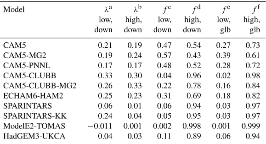
aver-Table 4.The fractional occurrences of low and high surface precipitation in PD cases over downdraft regimes (ω500>0 hPa day−1) and
global oceans andλunder these low and high surface precipitation situations only over downdraft regimes. Low precipitation situations refer to monthly surface precipitation rate (PRECL) less than 0.1 mm day−1while high precipitation situations refer to PRECL larger than
0.1 mm day−1.
Model λa λb fc fd fe ff
low, high, low, high, low, high, down down down down glb glb CAM5 0.21 0.19 0.47 0.54 0.27 0.73 CAM5-MG2 0.19 0.24 0.57 0.43 0.39 0.61 CAM5-PNNL 0.17 0.17 0.48 0.52 0.28 0.72 CAM5-CLUBB 0.33 0.30 0.04 0.96 0.02 0.98 CAM5-CLUBB-MG2 0.26 0.33 0.22 0.78 0.16 0.84 ECHAM6-HAM2 0.25 0.23 0.31 0.69 0.18 0.82 SPARINTARS 0.06 0.01 0.06 0.94 0.03 0.97 SPARINTARS-KK 0.24 0.04 0.05 0.95 0.03 0.97 ModelE2-TOMAS −0.011 0.001 0.002 0.998 0.001 0.999 HadGEM3-UKCA 0.04 0.03 0.11 0.89 0.06 0.94
aλunder low PRECL for downdraft regimes.bλunder high PRECL for downdraft regimes.
cFractional occurence of low PRECL for downdraft regimes.dFractional occurence of high PRECL for
downdraft regimes.eFractional occurence of low PRECL over all dynamical regimes.fFractional
occurence of high PRECL over all dynamical regimes.
aged surface precipitation rate less than 0.1 mm day−1)and
high precipitation (monthly averaged surface precipitation rate larger than 0.1 mm day−1). Table 4 lists the occurrence
frequency of each situation in different simulations. It shows that instances with low PRECL occurs much less often (from 2.2 % in CAM5-CLUBB to 38.8 % in CAM5-MG2) than those with high PRECL. The occurrence frequency of low precipitation situations is increased with the MG2 scheme (CAM5-MG2 and CAM5-CLUBB-MG2), compared with simulations without MG2. This increase is especially evident in CAM5-CLUBB (from 0.02 in CAM5-CLUBB to 0.16 in CAM5-CLUBB-MG2). This is consistent with Gettelman et al. (2015), who showed that surface precipitation decreases slightly in GCMs with MG2.
Note that low precipitation situations are only found in subsidence regimes (ω500>0 hPa day−1). Thus, the
sensitiv-ity of the LWP response to aerosol change under low and high precipitation is compared only in subsidence regimes. Table 4 also shows λ and the fractional occurrences of each precipitation situation in descending regimes. The frac-tional occurrence of low precipitation increases evidently in subsidence regimes, compared with that over global ocean. We find that the averages of λ under low precipita-tion are larger than those under high precipitaprecipita-tion in most models (CAM5, CAM5-PNNL, CAM5-CLUBB, ECHAM6-HAM2, SPRINTARS, SPRINTARS-KK and HadGEM3-UKCA) (Table 4). This result is different from some LES and single column model (SCM) results showing that smaller
λ values are found for low surface precipitation rather than high precipitation due to a decrease of LWP in response to increasing CCN (Ackerman et al., 2004; Guo et al., 2011). The decrease in LWP in these previous studies is found to
come from the entrainment drying due to increased entrain-ment from increasing aerosol loading (e.g., Bretherton et al., 2007) and this effect has not been explicitly included in most GCMs. Exceptions are CAM5 runs with the prognostic precipitation scheme MG2 (CAM5-MG2, CAM5-CLUBB-MG2). It can be seen from Table 4 that λ under low sur-face precipitation is smaller than under high precipitation only when MG2 scheme is used. It is still unclear what might cause this difference. It is interesting to note that λ
under low surface precipitation is still higher for HadGEM3-UKCA though a prognostic precipitation scheme is applied in HadGEM3-UKCA.
3.2.3 Shortwave cloud radiative effect
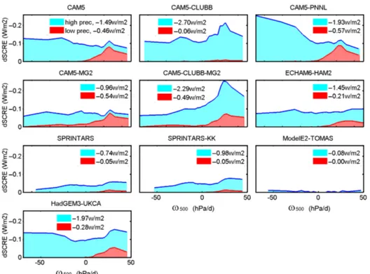
The shortwave cloud radiative effect (SCRE) is defined as the difference between all-sky and clear sky shortwave radiative fluxes at the top of atmosphere. Here SCRE is adjusted to the “clean-sky” SCRE, which is estimated as a diagnostic with aerosol optical depth set to zero (Ghan, 2013). Recent stud-ies on aerosol indirect effects mostly focus on stratocumulus clouds due to their significant cooling effect (e.g., Lu and Seinfeld, 2005; Bretherton et al., 2007). However, by sorting the change of SCRE (dSCRE) from PI to PD into dynamical regimes, our results suggest that the regimes of ascending motions are as important as the subsidence regimes and in some simulations dSCRE in ascending regimes is even larger than under subsidence regimes (e.g., CAM5-PNNL) (Fig. 7). This suggests that ascending regimes are crucial regimes in studying aerosol climate effect.
Figure 7.Change in shortwave cloud radiative effect (dSCRE, shown in blue line) from PI to PD as a function of dynamic regimes. Red patches are dSCRE contributed by low precipitation situations while blue patches are by high precipitation situations.
of dSCRE under a low and high precipitation situation). It is found that high precipitation situations constitute most of dSCRE (from 64 % in CAM5-MG2 to nearly 100 % in CAM5-CLUBB, Fig. 7) and the contributions from clouds with low precipitation rates are generally small, ranging from 0 to 36 %, due to their low occurrence frequency. dSCRE is reduced by 33 % for high precipitation situations from CAM5 to CAM5-MG2, and 15 % from CAM5-CLUBB to CAM5-CLUBB-MG2 (Fig. 7), consistent with the argument that prognostic precipitation schemes reduce aerosol indirect forcing (Posselt and Lohmann, 2009; Wang et al., 2012; Get-telman and Morrison, 2015). However, adopting a prognostic precipitation scheme is found to increase dSCRE under low precipitation situations. This is partly from the increase in the occurrence frequency of low precipitation instances when MG2 is adopted (Table 4).
Our sensitive tests indicate that results in Table 4 and Fig. 7 can be potentially sensitive to the precipitation thresh-old applied to separate high precipitation and low precipi-tation situations (not shown). The occurrence frequency of low precipitation situations increases with increasing thresh-old and the magnitude of increase can be different for dif-ferent models. For example, when the precipitation thresh-old increases from 0.01 to 0.20 mm day−1, the occurrence
frequency of low precipitation situations increases from 2 to 37 % in CAM5-PNNL while it increases from near 0 to 5 % in CAM5-CLUBB. Increasing the precipitation thresh-old also increases the contribution of low precipitation situ-ations to the total aerosol indirect forcing as the occurrence
frequency of low precipitation situations increases. However, our results indicate that the LWP response to aerosol per-turbations under low and high precipitation does not change much as the precipitation threshold changes and that high precipitation situations generally contribute more to the to-tal aerosol indirect forcing for precipitation threshold in the range of 0.01 to 0.20 mm day−1. More work is needed to
explore this further, such as how results may be different when instantaneous precipitation data (e.g., 3-hourly data) are used.
4 Summary
We have examined the regime-dependence of aerosol in-direct effects (AIE) over global oceans (from 60◦S to
60◦N) in several GCMs (CAM5, MG2,
CAM5-PNNL, CAM5-CLUBB, CAM5-CLUBB-MG2, ECHAM6-HAM2, SPRINTARS, SPRINTARS-KK, ModelE2-TOMAS and HadGEM3-UKCA). Model results are sorted into differ-ent dynamical regimes, characterized by the monthly mean mid-tropospheric 500 hPa vertical pressure velocity (ω500),
lower-tropospheric stability (LTS,θ700hPa–θsurface), and
sur-face precipitation rate.
aerosol cloud lifetime effect is regime-dependent. It is in strong ascending regimes and subsidence regimes thatλ dif-fers most between GCMs (Fig. 2a). Stratocumulus regimes have traditionally been the focus for studying aerosol indi-rect effects because of their significant cooling effect in cli-mate system (e.g., Ackerman et al., 2004; Bretherton et al., 2007; Gettelman et al., 2013). However, our results highlight that regimes with strong large-scale ascent should be another important regime to focus on in the future. Our results in-dicate that aerosol indirect forcing in regimes of vertical as-cent is close to, or even larger than that in low cloud regimes (Fig. 7). Note however that these GCMs do not treat aerosol effects in their representations of deep convection that dom-inates clouds and LWP in regimes with strong ascent, while new versions of CAM exist where a version of the MG mi-crophysics has been embedded in the deep convective param-eterization (Song and Zhang, 2011).
By adding LTS as another criterion, we further separated different low cloud types under large-scale subsidence and revealed some further differences in cloud lifetime effect of aerosols on different types of low clouds. For exam-ple, the large λ in subsidence regimes in CAM5-CLUBB and ECHAM6-HAM2 comes from both stratocumulus and trade wind cumulus, while in CAM5-CLUBB-MG2 it mostly comes from trade wind cumulus (Fig. 5). It is also interest-ing to note that the distribution of λ in SPRINTARS and SPRINTATSKK is more likely to depend on LTS rather than vertical pressure velocity.
Precipitation is another important factor in understanding simulated aerosol indirect forcing and its spread across mod-els. LWP is more sensitive to CCN change under low pre-cipitation situations (monthly mean surface prepre-cipitation rate less than 0.1 mm day−1)than under high precipitation
situ-ations (monthly mean surface precipitation rate larger than 0.1 mm day−1)in all models except for CAM5 simulations
with prognostic rain scheme (MG2) (Table 4). Results de-rived from large eddy simulation (LES) and single column model (SCM) (e.g., Ackerman et al., 2004; Guo et al., 2011) have shown thatλcould be negative under low precipitation situations, which indicates that λis expected to be smaller under low precipitation situations. Further efforts are needed to understand the differences among different models and the difference between global model results and results from process-level studies.
Our results indicate that grids with high precipitation con-tribute most to aerosol indirect forcing (from 64 % in CAM5-MG2 to nearly 100 % in CAM5-CLUBB, Fig. 7) and the contributions from model grids with low precipitation are relatively small, ranging from 0 to 36 %. Adding prognos-tic precipitation scheme (MG2) reduces the shortwave cloud radiative effect (SCRE) for high precipitation situations. As low precipitation situations are much less prevalent than high precipitation situations, total SCRE decreases in models with prognostic rain scheme compared to those with a diagnostic rain scheme.
Appendix A: Global aerosol-climate models
CAM5: This is the default version of CAM5.3. The moist turbulence scheme is based on Bretherton and Park (2009), which explicitly simulates stratus- radiation-turbulence in-teractions. The shallow convection scheme is from Park and Bretherton (2009) and the deep convection parameterization is retained from CAM4.0 (Neale et al., 2008). The two-moment cloud microphysics scheme from Morrison and Get-telman (2008) (MG) is used to predict both the mass and number mixing ratios for cloud water and cloud ice with a diagnostic formula for rain and snow. The cloud ice micro-physics was further modified to allow ice supersaturation and aerosol effects on ice clouds (Gettelman et al., 2010). The activation of aerosol particles into cloud droplets is param-eterized by Abdul-Razzak and Ghan (2000, hereafter ARG) and the autoconversion scheme is based on Khairoutdinov and Kogan (2000) (KK). A modal approach is used to treat aerosols in CAM5 (Liu et al., 2012a; Ghan et al., 2012). Aerosol size distribution can be represented by using either 3 modes or 7 modes, and the default 3-mode treatment is used in this study. Simulations were performed at 1.9◦
×2.5◦ hor-izontal resolution with finite volume dynamical core, using 30 vertical levels.
CAM5-PNNL: This is the same as CAM5, but a new unified treatment of vertical transport and in-cloud wet re-moval processes in convective clouds developed by Wang et al. (2013) is applied. It has a more detailed treatment of aerosol activation in convective updrafts and a mechanism is added for laterally entrained aerosols to be activated and then removed. In addition, a few other changes have been introduced to stratiform cloud wet scavenging processes in CAM5-PNNL to improve the fidelity of the aerosol simula-tion, including the vertical distribution of aerosols and their transport to remote regions (Wang et al., 2013).
CAM5-MG2: This is the same as CAM5, but the original two-moment MG scheme with diagnostic treatment for rain and snow in CAM5 is replaced by the updated MG scheme (MG2) with prognostic scheme for rain and snow (Gettelman et al., 2015).
CAM5-CLUBB: This is the same as CAM5, but the sep-arate treatments of boundary layer turbulence, large-scale cloud macrophysics and shallow convection in CAM5 is re-placed by CLUBB, a higher-order turbulence closure that unifies these different treatments (Bogenschutz et al., 2013). This therefore includes aerosol effects on shallow convec-tion.
CLUBB-MG2: This is the same as CAM5-CLUBB, but the MG2 scheme with prognostic rain and snow treatment replaces the original MG scheme with diagnostic rain and snow treatment (Gettelman et al., 2015). This also includes aerosol effects on shallow convection.
ECHAM6-HAM2: ECHAM-HAMMOZ (echam6.1-ham2.2-moz0.9) is a global aerosol-chemistry climate model. In this study only the global aerosol-climate model
part of ECHAM-HAMMOZ is used and for the sake of brevity referred to as ECHAM6-HAM2 (Neubauer et al., 2014). It consists of the general circulation model ECHAM6 (Stevens et al., 2013) coupled to the latest version of the aerosol module HAM2 (Stier et al., 2005; Zhang et al., 2012) and uses a two-moment cloud microphysics scheme that includes prognostic equations for the cloud droplet and ice crystal number concentrations as well as cloud water and cloud ice (Lohmann et al., 2007; Lohmann and Hoose, 2009). The activation of aerosol articles into cloud droplets is parameterized by Lin and Leaitch (1997) and the autoconversion scheme is based on the KK scheme. Cumulus convection is represented by the parameterization of Tiedtke (1989) with modifications by Nordeng (1994) for deep convection. Aerosol effects on convective clouds are not included, but there is a dependence of cloud droplets detrained from convective clouds on aerosol. Simulations were performed at T63 (1.9◦×1.9◦) spectral resolution
using 31 vertical levels (L31).
SPRINTARS: SPRINTARS (Takemura et al., 2005) is a global aerosol transport-climate model based on a gen-eral circulation model, MIROC (Watanabe et al., 2010). In this study, the horizontal and vertical resolutions are T106 (1.125◦×approx. 1.125◦) and 56 layers, respectively.
SPRINTARS is coupled with the radiation and cloud micro-physics schemes in MIROC to calculate the aerosol-radiation and aerosol–cloud interactions. A prognostic scheme for de-termining the cloud droplet and ice crystal number concen-trations is introduced (Takemura et al., 2009). The default autoconversion scheme in MIROC-SPRINTARS is based on Berry (1968), and the activation of aerosol particles into cloud droplet is based on the ARG scheme.
SPRINTARS-KK: This is the same as SPRINTARS, but the default autoconversion scheme in SPRINTARS is re-placed with the KK autoconversion scheme.
ModelE2-TOMAS: ModelE2-TOMAS is a global-scale atmospheric chemistry-climate model, which consists of the state-of-the-art NASA GISS ModelE2 general circulation model (Schmidt et al., 2014) coupled to the TwO-Moment Aerosol Sectional (TOMAS) microphysics model (Lee and Adams, 2012; Lee et al., 2015). ModelE2-TOMAS has 2◦
latitude by 2.5◦ longitude resolution, with 40 vertical
veloc-ity that is computed based on a large-scale vertical velocveloc-ity and sub-grid velocity.
HadGEM3-UKCA: HadGEM3-UKCA is a global compo-sition climate model (http://www.ukca.ac.uk). It consists of the third generation of the Hadley Centre Global Environ-mental Model (Hewitt et al., 2011) developed at the UK Met Office. This general circulation model is non-hydrostatic and uses a semi-Lagrangian transport scheme. We are using the atmospheric configuration: General Atmosphere (GA) 4.0 as documented in Walters et al., (2014), except for the addition of the UKCA aerosol and chemistry scheme which is fully coupled with the radiation scheme of HadGEM3 (Bellouin et al., 2013). UKCA is a two-moment pseudo-modal scheme which carries both aerosol number concentration and compo-nent mass as prognostic tracers. It calculates the evolution of five aerosol species, sulfate, particulate organic matter, black carbon, sea salt and dust, in both internally and externally
mixed particles. The aerosol scheme in UKCA is based on the Global Model of Aerosol Processes (GLOMAP-mode, Mann et al., 2010). The main exception is that dust is cal-culated separately using 6 size bins. UKCA hence only con-siders 5 modes. The tropospheric chemistry part of UKCA is described in O’Connor et al. (2014). HadGEM3 uses a prognostic treatment of rain formulation (Abel and Boutle, 2012) and employs a prognostic cloud fraction and conden-sation cloud scheme (PC2) (Wilson et al., 2008), in which the cloud droplet number concentration is diagnosed from the expected number of aerosols that are available to activate at each timestep (West et al., 2014). Cumulus convection is represented by a mass flux convection scheme based on Gre-gory and Rowntree (1990) with various extensions (Walters et al., 2014). Simulations were performed at N96L85 reso-lution, a regular 1.25◦latitude×1.875◦longitude grid in the
Acknowledgements. M. Wang acknowledged the support from the Jiangsu Province Specially-appointed professorship grant and the One Thousand Young Talents Program and the National Natural Science Foundation of China (41575073). The contribution from Pacific Northwest National Laboratory was supported by the US Department of Energy (DOE), Office of Science, Decadal and Regional Climate Prediction using Earth System Models (EaSM program). H. Wang acknowledges support by the DOE Earth System Modeling program. The Pacific Northwest National Laboratory is operated for the DOE by Battelle Memorial Institute under contract DE-AC06-76RLO 1830. The ECHAM-HAMMOZ model is developed by a consortium composed of ETH Zurich, Max Planck Institut für Meteorologie, Forschungszentrum Jülich, University of Oxford, the Finnish Meteorological Institute and the Leibniz Institute for Tropospheric Research, and managed by the Center for Climate Systems Modeling (C2SM) at ETH Zurich. D. Neubauer gratefully acknowledges the support by the Austrian Science Fund (FWF): J 3402-N29 (Erwin Schrödinger Fellowship Abroad). The Center for Climate Systems Modeling (C2SM) at ETH Zurich is acknowledged for providing technical and scientific support. This work was supported by a grant from the Swiss National Supercomputing Centre (CSCS) under project ID s431. D. G. Partridge would like to acknowledge support from the UK Natural Environment Research Council project ACID-PRUF (NE/I020148/1) as well as thanks to N. Bellouin for useful discussions during the course of this work. The development of GLOMAP-mode within HadGEM is part of the UKCA project, which is supported by both NERC and the Joint DECC/Defra Met Office Hadley Centre Climate Programme (GA01101). We acknowledge use of the MONSooN system, a collaborative facility supplied under the Joint Weather and Climate Research Programme, a strategic partnership between the Met Office and the Natural Environment Research Council. P. Stier would like to acknowledge support from the European Research Council under the European Union’s Seventh Framework Programme (FP7/2007-2013) / ERC grant agreement no. FP7-280025. Edited by: P. Chuang
References
Abel, S. J. and Boutle, I. A.: An improved representation of the rain-drop size distribution for single-moment microphysics schemes, Q. J. Roy. Meteor. Soc., 138, 2151–2162, doi:10.1002/qj.1949, 2012.
Abdul-Razzak, H. and Ghan, S. J.: A parameterization of aerosol activation 2. Multiple aerosol types, J. Geophys. Res., 105, 6837– 6844, 2000.
Ackerman, A. S., Kirkpatrick, M. P., Stevens, D. E., and Toon, O. B.: The impact of humidity above stratiform clouds on indirect aerosol climate forcing, Nature, 432, 1014–1017, doi:10.1038/nature03174, 2004.
Albrecht, B. A.: Aerosols, cloud microphysics, and fractional cloudiness, Science, 245, 1227–1230, doi:10.1126/science.245.4923.1227, 1989.
Andreae, M. O., Rosenfeld, D., Artaxo, P., Costa, A. A., Frank, G. P., Longo, K. M., and Silva-Dias, M. A. F.:
Smok-ing rain clouds over the Amazon, Science, 303, 1337–1342, doi:10.1126/science.1092779, 2004.
Bellouin, N., Mann, G. W., Woodhouse, M. T., Johnson, C., Carslaw, K. S., and Dalvi, M.: Impact of the modal aerosol scheme GLOMAP-mode on aerosol forcing in the Hadley Centre Global Environmental Model, Atmos. Chem. Phys., 13, 3027– 3044, doi:10.5194/acp-13-3027-2013, 2013.
Berry, E. X.: Modification of the warm rain process, Proc. First Natl. Conf. Weather Modification, American Meteorological Society, State University of New York, Albany, 81–88, 1968.
Bogenschutz, P. A., Gettelman, A., Morrison, H., Larson, V. E., Craig, C., and Schanen, D. P.: Higher-Order Turbulence Closure and Its Impact on Climate Simulations in the Community Atmo-sphere Model, J. Climate, 26, 9655–9676, doi:10.1175/jcli-d-13-00075.1, 2013.
Bony, S. and Dufresne, J. L.: Marine boundary layer clouds at the heart of tropical cloud feedback uncertainties in climate models, Geophys. Res. Lett., 32, L20806, doi:10.1029/2005gl023851, 2005.
Bony, S., Dufresne, J. L., Le Treut, H., Morcrette, J. J., and Se-nior, C.: On dynamic and thermodynamic components of cloud changes, Clim. Dynam., 22, 71–86, doi:10.1007/s00382-003-0369-6, 2004.
Boucher, O., Randall, D., Artaxo, P., Bretherton, C., Feingold, G., Forster, P., Kerminen, V.-M., Kondo, Y., Liao, H., Lohmann, U., Rasch, P., Satheesh, S. K., Sherwood, S., Stevens, B., and Zhang, X. Y.: Clouds and Aerosols, in: Climate Change 2013: The Phys-ical Science Basis. Contribution of Working Group I to the Fifth Assessment Report of the Intergovernmental Panel on Climate Change, edited by: Stocker, T. F., Qin, D., Plattner, G.-K., Tignor, M., Allen, S. K., Boschung, J., Nauels, A., Xia, Y., Bex V., and Midgley, P. M., Cambridge University Press, Cambridge, United Kingdom and New York, NY, USA, 2013.
Bretherton, C. S. and Park, S.: A New Moist Turbulence Parame-terization in the Community Atmosphere Model, J. Climate, 22, 3422–3448, doi:10.1175/2008jcli2556.1, 2009.
Bretherton, C. S., Blossey, P. N., and Uchida, J.: Cloud droplet sedimentation, entrainment efficiency, and subtropi-cal stratocumulus albedo, Geophys. Res. Lett., 34, L03813, doi:10.1029/2006gl027648, 2007.
Chen, Y.-C., Christensen, M. W., Stephens, G. L., and Seinfeld, J. H.: Satellite-based estimate of global aerosol-cloud radia-tive forcing by marine warm clouds, Nat. Geosci., 7, 643–646, doi:10.1038/ngeo2214, 2014.
Coakley, J. A. and Walsh, C. D.: Limits to the aerosol in-direct radiative effect derived from observations of ship tracks, J. Atmos. Sci., 59, 668–680, doi:10.1175/1520-0469(2002)059<0668:lttair>2.0.co;2, 2002.
Del Genio, A. D. and Yao, M.-S.: Efficient cumulus parameteriza-tion for long-term climate studies: The GISS scheme, in: The Representation of Cumulus Convection in Numerical Models, AMS Meteorol. Monogr., Vol. 46, edited by: Emanuel, K. A. and Raymond, D. A., 181–184, Am. Meteorol. Soc., Washing-ton D.C., 1993.
Del Genio, A. D., Yao, M. S., Kovari, W., and Lo, K. K.: A prognos-tic cloud water parameterization for general circulation models, J. Climate, 9, 270–304, 1996.
Comparison with Other Schemes, J. Climate, 28, 1268–1287, doi:10.1175/JCLI-D-14-00102.1, 2015.
Gettelman, A., Liu, X., Ghan, S. J., Morrison, H., Park, S., Con-ley, A. J., Klein, S. A., Boyle, J., Mitchell, D. L., and Li, J. L. F.: Global simulations of ice nucleation and ice super-saturation with an improved cloud scheme in the Community Atmosphere Model, J. Geophys. Res.-Atmos., 115, D18216, doi:10.1029/2009jd013797, 2010.
Gettelman, A., Morrison, H., Terai, C. R., and Wood, R.: Micro-physical process rates and global aerosol–cloud interactions, At-mos. Chem. Phys., 13, 9855–9867, doi:10.5194/acp-13-9855-2013, 2013.
Gettelman, A., Morrison, H., Santos, S., Bogenschutz, P., and Caldwell, P. M.: Advanced Two-Moment Bulk Micro-physics for Global Models. Part II: Global Model Solutions and Aerosol–Cloud Interactions, J. Climate, 28, 1288–1307, doi:10.1175/JCLI-D-14-00103.1, 2015.
Ghan, S. J.: Technical Note: Estimating aerosol effects on cloud radiative forcing, Atmos. Chem. Phys., 13, 9971–9974, doi:10.5194/acp-13-9971-2013, 2013.
Ghan, S. J., Liu, X., Easter, R. C., Zaveri, R., Rasch, P. J., Yoon, J. H., and Eaton, B.: Toward a Minimal Representation of Aerosols in Climate Models: Comparative Decomposition of Aerosol Di-rect, SemidiDi-rect, and Indirect Radiative Forcing, J. Climate, 25, 6461–6476, 10.1175/jcli-d-11-00650.1, 2012.
Ghan, S., Wang, M., Zhang, S., Ferrachat, S., Gettelman, A., Gries-feller, J., Kipling, Z., Lohmann, U., Morrison, H., Neubauer, D., Partridge, D. G., Stier, P., Takemura, T., Wang, H., and Zhang, K.: Challenges in constraining anthropogenic aerosol effects on cloud radiative forcing using present-day spatiotemporal vari-ability, P. Natl. Acad. Sci. USA, doi:10.1073/pnas.1514036113, online first, 2016.
Gregory, D. and Rowntree, P. R.: A massflux convection scheme with representation of cloud ensemble characteristics and sta-bility dependent closure, Mon. Weather Rev., 118, 1483–1506, doi:10.1175/1520-0493(1990)118<1483:AMFCSW>2.0.CO;2, 1990.
Gryspeerdt, E. and Stier, P.: Regime-based analysis of aerosol-cloud interactions, Geophys. Res. Lett., 39, L21802, doi:10.1029/2012gl053221, 2012.
Gryspeerdt, E., Stier, P., and Grandey, B. S.: Cloud fraction me-diates the aerosol optical depth-cloud top height relationship, Geophys. Res. Lett., 41, 3622–3627, doi:10.1002/2014gl059524, 2014a.
Gryspeerdt, E., Stier, P., and Partridge, D. G.: Links between satellite-retrieved aerosol and precipitation, Atmos. Chem. Phys., 14, 9677–9694, doi:10.5194/acp-14-9677-2014, 2014b. Gryspeerdt, E., Stier, P., and Partridge, D. G.: Satellite
observa-tions of cloud regime development: the role of aerosol processes, Atmos. Chem. Phys., 14, 1141–1158, doi:10.5194/acp-14-1141-2014, 2014c.
Guo, H., Golaz, J. C., and Donner, L. J.: Aerosol effects on stratocu-mulus water paths in a PDF-based parameterization, Geophys. Res. Lett., 38, L17808, doi:10.1029/2011gl048611, 2011. Guo, H., Golaz, J. C., Donner, L. J., Wyman, B., Zhao, M., and
Ginoux, P.: CLUBB as a unified cloud parameterization: Op-portunities and challenges, Geophys. Res. Lett., 42, 4540–4547, doi:10.1002/2015GL063672, 2015.
Guo, Z., Wang, M. H., Qian, Y., Larson, V. E., Ghan, S., Ovchin-nikov, M., Bogenschutz, P. A., Gettelman, A., and Zhou, T. J.: Parametric behaviors of CLUBB in simulations of low clouds in the Community Atmosphere Model (CAM), J. Adv. Model. Earth Syst., 7, 1005–1025, doi:10.1002/2014ms000405, 2015. Hewitt, H. T., Copsey, D., Culverwell, I. D., Harris, C. M., Hill, R.
S. R., Keen, A. B., McLaren, A. J., and Hunke, E. C.: Design and implementation of the infrastructure of HadGEM3: the next-generation Met Office climate modelling system, Geosci. Model Dev., 4, 223–253, doi:10.5194/gmd-4-223-2011, 2011.
IPCC: Climate Change 2013: The Physical Science Basis. Contri-bution of Working Group I to the Fifth Assessment Report of the Intergovernmental Panel on Climate Change, edited by: Stocker, T. F., Qin, D., Plattner, G.-K., Tignor, M., Allen, S. K., Boschung, J., Nauels, A., Xia, Y., Bex, V., and Midgley, P. M., Cambridge University Press, Cambridge, United Kingdom and New York, NY, USA, 1535 pp., 2013
Kaufman, Y. J., Koren, I., Remer, L. A., Rosenfeld, D., and Rudich, Y.: The effect of smoke, dust, and pollution aerosol on shallow cloud development over the Atlantic Ocean, P. Natl. Acad. Sci. USA, 102, 11207–11212, doi:10.1073/pnas.0505191102, 2005. Khairoutdinov, M. and Kogan, Y.: A new cloud physics
parame-terization in a large-eddy simulation model of marine stratocu-mulus, Mon. Weather Rev., 128, 229–243, doi:10.1175/1520-0493(2000)128<0229:ancppi>2.0.co;2, 2000.
Kooperman, G. J., Pritchard, M. S., Ghan, S. J., Wang, M. H., Somerville, R. C. J., and Russell, L. M.: Constraining the in-fluence of natural variability to improve estimates of global aerosol indirect effects in a nudged version of the Community Atmosphere Model 5, J. Geophys. Res.-Atmos., 117, D23204, doi:10.1029/2012jd018588, 2012.
Lamarque, J.-F., Bond, T. C., Eyring, V., Granier, C., Heil, A., Klimont, Z., Lee, D., Liousse, C., Mieville, A., Owen, B., Schultz, M. G., Shindell, D., Smith, S. J., Stehfest, E., Van Aar-denne, J., Cooper, O. R., Kainuma, M., Mahowald, N., Mc-Connell, J. R., Naik, V., Riahi, K., and van Vuuren, D. P.: His-torical (1850–2000) gridded anthropogenic and biomass burning emissions of reactive gases and aerosols: methodology and ap-plication, Atmos. Chem. Phys., 10, 7017–7039, doi:10.5194/acp-10-7017-2010, 2010.
Lebo, Z. J. and Feingold, G.: On the relationship between re-sponses in cloud water and precipitation to changes in aerosol, Atmos. Chem. Phys., 14, 11817–11831, doi:10.5194/acp-14-11817-2014, 2014.
Lee, Y.-H. and Adams, P. J.: A fast and efficient version of the TwO-Moment Aerosol Sectional (TOMAS) global aerosol microphysics model, Aerosol. Sci. Tech., 46, 678–689, doi:10.1080/02786826.2011.643259, 2012.
Lee, Y. H., Adams, P. J., and Shindell, D. T.: Evaluation of the global aerosol microphysical ModelE2-TOMAS model against satellite and ground-based observations, Geosci. Model Dev., 8, 631–667, doi:10.5194/gmd-8-631-2015, 2015.
Lin, H. and Leaitch, W. R.: Development of an in-cloud aerosol ac-tivation parameterization for climate modelling, in: Proceedings of the WMO Workshop on Measurement of Cloud Properties for Forecasts of Weather, Air Quality and Climate, World Meteorol. Organ., Geneva, 328–335, 1997.