www.geosci-model-dev.net/7/2867/2014/ doi:10.5194/gmd-7-2867-2014
© Author(s) 2014. CC Attribution 3.0 License.
Sensitivity of simulated CO
2
concentration to regridding of global
fossil fuel CO
2
emissions
X. Zhang1, K. R. Gurney1,2, P. Rayner3, Y. Liu4, and S. Asefi-Najafabady1
1School of Life Sciences, Arizona State University, Tempe, AZ 85287, USA
2Global Institute of Sustainability, Arizona State University, Tempe, AZ 85287, USA 3School of Earth Sciences, University of Melbourne, 3010, Victoria, Australia
4Laboratory for Atmosphere, Science Systems and Applications, Inc., NASA Goddard Space Flight Center Code 614,
Greenbelt, MD 20771, USA
Correspondence to:X. Zhang ([email protected])
Received: 13 March 2014 – Published in Geosci. Model Dev. Discuss.: 3 June 2014 Revised: 5 October 2014 – Accepted: 15 October 2014 – Published: 4 December 2014
Abstract. Errors in the specification or utilization of fos-sil fuel CO2emissions within carbon budget or atmospheric
CO2 inverse studies can alias the estimation of biospheric
and oceanic carbon exchange. A key component in the sim-ulation of CO2concentrations arising from fossil fuel
emis-sions is the spatial distribution of the emission near coast-lines. Regridding of fossil fuel CO2emissions (FFCO2)from
fine to coarse grids to enable atmospheric transport simula-tions can give rise to mismatches between the emissions and simulated atmospheric dynamics which differ over land or water. For example, emissions originally emanating from the land are emitted from a grid cell for which the vertical mix-ing reflects the roughness and/or surface energy exchange of an ocean surface. We test this potential “dynamical inconsis-tency” by examining simulated global atmospheric CO2
con-centration driven by two different approaches to regridding fossil fuel CO2 emissions. The two approaches are as
fol-lows: (1) a commonly used method that allocates emissions to grid cells with no attempt to ensure dynamical consistency with atmospheric transport and (2) an improved method that reallocates emissions to grid cells to ensure dynamically con-sistent results. Results show large spatial and temporal dif-ferences in the simulated CO2concentration when
compar-ing these two approaches. The emissions difference ranges from −30.3 TgC grid cell−1yr−1 (−3.39 kgC m−2yr−1)
to +30.0 TgC grid cell−1yr−1 (+2.6 kgC m−2yr−1) along
coastal margins. Maximum simulated annual mean CO2
con-centration differences at the surface exceed ±6 ppm at var-ious locations and times. Examination of the current CO2
monitoring locations during the local afternoon, consistent with inversion modeling system sampling and measurement protocols, finds maximum hourly differences at 38 stations exceed ±0.10 ppm with individual station differences ex-ceeding−32 ppm. The differences implied by not accounting for this dynamical consistency problem are largest at moni-toring sites proximal to large coastal urban areas and point sources. These results suggest that studies comparing simu-lated to observed atmospheric CO2concentration, such as
at-mospheric CO2inversions, must take measures to correct for
this potential problem and ensure flux and dynamical consis-tency.
1 Introduction
The terrestrial biosphere and oceans play a critical role in the global carbon cycle by removing approximately 5.1 PgC yr−1of CO2out of the total emitted due to industrial
activity and deforestation (Le Quéré et al., 2013). Quantifica-tion of the spatial and temporal patterns of this removal using atmospheric CO2inversions is an important approach for
un-derstanding the feedbacks between the carbon cycle and the climate system (e.g., Gurney et al., 2002). Atmospheric CO2
inversions infer the ocean and biosphere uptake by solving a set of source–receptor relationships, with the fossil fuel CO2
Global fossil fuel CO2emission data products are now
be-ing produced at spatial resolutions smaller than 10 km and time resolutions that resolve the diurnal cycle (Rayner et al., 2010; Oda and Maksyutov, 2011; Wang et al., 2013; Nassar et al., 2013). This, along with the increasing density of at-mospheric CO2concentration observations, places new
em-phasis on a careful examination of the use and uncertainty associated with these high-resolution fossil fuel CO2
emis-sion data products (Ciais et al., 2010; Gurney et al., 2005; Peylin et al., 2011; Nassar et al., 2013; Asefi-Najafabady et al., 2014). For example, Gurney et al. (2005) found a monthly regional bias of up to 50 % in the biosphere’s net carbon ex-change caused by unaccounted variation in fossil fuel emis-sions. Peylin et al. (2011) also showed a large response in simulated CO2 concentration to the spatial and temporal
resolution of fossil fuel emissions over Europe. Similarly, Nassar et al. (2013) confirmed the importance of hourly and weekly cycles in fossil fuel emissions to simulated CO2
con-centration levels. It is clear from these studies that the speci-fication of the fossil fuel CO2emissions is a critical
compo-nent in efforts that use fossil fuel emissions either directly or as part of an atmospheric CO2inversion process.
In addition to concerns regarding the accuracy of the high-resolution fossil fuel CO2emission data products, there are
elements of uncertainty in how they are used within atmo-spheric tracer transport schemes, either in forward simulation or inverse mode. Transport models typically distinguish the surface characteristics of a model grid cell in broad classes such as land versus water or urban versus rural. These clas-sifications are important to both the emissions of fossil fuel CO2(FFCO2) and atmospheric transport above and/or
down-wind of particular grid cells. For example, modeled atmo-spheric transport processes such as mixing with the planetary boundary layer, convection, synoptic flow, and even general circulation are influenced by the grid cell surface character-istics (e.g., surface roughness or energy budget).
Global tracer transport models usually discretize surface grid cells at a lower resolution than those of fossil fuel CO2
emission data products produced in recent years and, thus, the emissions need to be aggregated to the coarser model resolution. In this process, the transport model grid cells with less than 50 % land geography are usually designated as water grid cells. Emissions present on the finer FFCO2
grid, resident within the coarser model water grid cell, are thereby mixed into the atmosphere according to vertical mix-ing characteristics of ocean or lake transport dynamics. This inconsistency between the emissions and transport dynamics can cause bias both locally and downwind of the errant grid cell(s). This problem is particularly important for fossil fuel CO2 emissions as they are notoriously large along coastal
margins where population and infrastructure are dominant. This study aims to quantify this bias arising from the re-gridding of fossil fuel CO2emissions in global tracer
trans-port simulations. The bias is defined as spatial distribution and temporal variations of the simulated CO2concentration
difference driven with two regridded fossil fuel emission inventories. We do this by constructing two experiments: (1) using the typical regridding procedure in which emis-sions are left in grid cells defined by the majority surface ge-ography and (2) proportionally shifting or “shuffling” these emissions to neighboring land grid cells to maintain the spa-tial integrity of the fossil fuel emissions while avoiding the emissions–transport inconsistency
Although a similar phenomenon might be expected for in-land urban areas where designation of urban versus rural grid cells may not align with surface emissions, the global tracer transport models used in this study do not attempt to resolve transport dynamics over urban versus rural areas.
Thus, we restrict ourselves to the study of the land versus water misallocation problem.
Section 2 describes the fossil fuel CO2emission data
prod-uct used in the simulations, the atmospheric transport model employed and the adjustment method used to regrid the emis-sions. Section 3 presents results highlighting the difference induced by the shuffling procedure. We examine differences in emissions and in concentrations, the latter performed at active CO2monitoring locations for which the shuffling
in-fluence is greatest. Section 4 presents our conclusions.
2 Methods
The impact of fossil fuel CO2emission regridding is tested
here by examination of simulated CO2concentration driven
by two different emission fields through an atmospheric transport model. The fossil fuel CO2 emissions are
aggre-gated from a 0.1◦×0.1◦ grid to a 1.25◦×1.0◦ transport model grid. One of these emission fields has the coastal grid cells “shuffled” to correct for the regridding impact (“exper-iment”) while the other is left in the original unshuffled con-dition (“control”).
2.1 Fossil fuel CO2emissions
Fossil fuel CO2emissions from the Fossil Fuel Data
Assimi-lation System (FFDAS) version 2.0 are used as the fossil fuel CO2emissions in this study (Asefi-Najafabady et al., 2014).
The FFDAS emissions are produced on a 0.1◦×0.1◦grid for every year spanning the 1997 to 2010 time period. We use emissions for 2002 in this study. The FFDAS is a data assim-ilation system that estimates the fossil fuel CO2 emissions
In-ternational Energy Agency (IEA), and a recently constructed database of global power plant CO2 emissions (Elvidge et
al., 2009; Asefi-Najafabady et al., 2014).
FFDAS version 2.0 originally estimates fossil fuel CO2
emissions at 0.1◦and annual resolutions over the globe. From this product, we have derived a fossil fuel CO2emission
dis-tribution suitable for the use with our model by dividing the annual amounts in each grid cell by 2920 to obtain emissions that are evenly distributed in time, at the temporal resolution of our model (i.e., 3 h).
2.2 Atmospheric transport model
This study uses a global tracer transport model – the Pa-rameterized Chemical Transport Model (PCTM) – to sim-ulate the CO2concentration resulting from the FFDAS
sur-face emissions (Kawa et al., 2004, 2010). The model uses dynamical fields from the Modern-Era Retrospective anal-ysis for Research and Applications (MERRA) (Bosilovich, 2013), which is a NASA reanalysis for the satellite era us-ing a new version of the Goddard Earth Observus-ing System Data Assimilation System Version 5 (GEOS-5). The initial data product of GEOS-5 is at 0.7◦longitude×0.5◦latitude with 72 hybrid vertical levels. Two coarser MERRA prod-ucts are also produced by aggregating the high-resolution product to a resolution at 1.25◦longitude×1.25◦latitude or 1.25◦longitude×1◦ latitude with 72 hybrid vertical levels (Rienecker et al., 2011; Reichle et al., 2011; Reichle, 2012). In atmospheric transport simulation and inversion system, a dynamical consistence problem might be introduced if the driving meteorology data do not match the transport model grid. However, this problem does not exist in this study, since the MERRA product used in this study is on the same grid as PCTM. The model uses a semi-Lagrangian advec-tion scheme; the subgrid-scale transport includes convecadvec-tion and boundary layer turbulence processes. The model is run at 1.25◦longitude×1.0◦latitude with 72 hybrid vertical levels. The vertical mixing profile in PCTM includes two dynami-cal processes: turbulent diffusion in the boundary layer and convection. The two processes are parameterized following the MERRA model – which differentiates the vertical mixing in the boundary layer over land and ocean by using differ-ent surface heating, radiation, moisture, roughness and other physical factors in the eddy diffusion coefficient (Kh scheme) (Louis et al., 1982; Lock et al., 2000; McGrath-Spangler and Molod, 2014). Considering the purpose of this study, a check of the diffusion coefficients of the MERRA meteorology is performed. The result shows a significant difference between land and ocean planetary boundary layers, indicating the ex-istence of different vertical mixing characteristics between the two boundaries (Fig. 1).
The simulation is run for 4 years, driven by 2002 MERRA meteorology and fossil fuel CO2 surface emissions
(cy-cled repeatedly). The MERRA meteorology has a 3 h time resolution, and a 7.5 min time step is used in the model
Figure 1.Daily mean diffusion coefficient (KH) at 1.25◦×1.0◦for 30 July 2002 at pressure level about∼950 hpa in MERRA reanal-ysis. The diffusion coefficient is determined using aK-diffusion scheme in MERRA modeling.
simulations. There is no time structure in the fossil fuel emis-sions. In the model simulations, tracers are propagated in the atmosphere to reach a state of equilibrium under the ap-plied forcing. This is achieved with a 4-year simulation in which the first 3-year period is used for spin-up and the last year is used for analysis. The PCTM outputs hourly CO2 concentration at every point in the three-dimensional
grid. The annual mean surface CO2 concentration field
and hourly time series at GLOBALVIEW-CO2
monitor-ing sites are analyzed (http://www.esrl.noaa.gov/gmd/ccgg/ globalview/) (Masarie and Tans, 1995).
2.3 Coastal “shuffling”
The FFDAS emissions are regridded from the original 0.1◦×0.1◦resolution to the 1.25◦longitude×1.0◦latitude resolution of the PCTM. The two grids have the same ori-gin, and hence the coarser grid is overlaid onto the finer grid and the 0.1◦grid cells are integrated, as needed. In the longi-tudinal direction, grid cell boundaries do not align, so area-weighting was used to distribute emissions.
mag-Figure 2.Depiction of the “shuffling” procedure when regridding from a 0.1◦×0.1◦to a 1.25◦×1.0◦model grid. Capital black let-ters denote the coarser model grid (1.25◦×1.0◦). Grid cells out-lined with dashed lines denote the finer model grid (0.1◦×0.1◦). Green denotes land, and blue denotes water. Example emission val-ues and weighting valval-ues (w)and the direction of the allocation are included.
nitude of those adjacent land grid cells (Fig. 2). The weight is defined as the ratio of emissions in each of the designated adjacent grid cells to the sum of their emissions:
wj =Fj/ N
X
i=1
Fi, (1)
where wj is the weight of thejth land grid cell, Fj is its emissions, and N is the total number of land grid cells to which emissions are transferred. Adjacent grid cells are de-fined as those that share a corner with the shuffled cell.
3 Results and discussion
3.1 Emissions difference
The shuffling procedure reallocates emissions along global coastlines, but the impact on the final CO2 fluxes is most
pronounced where there are large coastal emissions associ-ated with urban areas or large point sources. Figure 3 shows the difference in surface emissions between the control and experiment emission fields. The coastal locations with cities or large point sources exhibit an emissions “dipole”. Positive values reflect the addition of emissions to land grid cells adja-cent to those designated as ocean in the coarse grid land–sea mask while negative values reflect the removal of emissions from grid cells designated as ocean.
Figure 3. Difference between experiment and control fossil fuel CO2emissions. The difference is obtained by subtracting the con-trol from the experiments. The emission values for some grid cells are not evident because the grid cells are saturated (beyond the color scale range).
The largest emissions adjustments occur in coastal ar-eas of the US Great Lakes, coastal Europe, China, India and Japan. The range of the emission difference varies from −30.3 TgC grid cell−1yr−1 (−3.39 kgC m−2yr−1)
to +30.0 TgC grid cell−1yr−1 (+2.6 kgC m−2yr−1). To
provide context, an emission difference of 30 TgC grid cell−1yr−1 is equivalent to ∼62 and ∼13 % of the
annual total carbon emissions for the Netherlands and Germany in 2002, respectively, but is only limited to a few grid cells in eastern Asia. Most emission differences in land grid cells vary between 0.001 TgC grid cell−1yr−1 (0.0001 kgC m−2yr−1) and 5.0 TgC grid cell−1yr−1 (0.056 kgC m−2yr−1). The summed magnitude of the emissions that are relocated from ocean to neighboring land grid cells is 674.5 TgC yr−1, which is equivalent to ∼10% of the global total fossil fuel CO2emissions in 2002.
3.2 CO2concentration difference
The atmospheric CO2concentration resulting from the
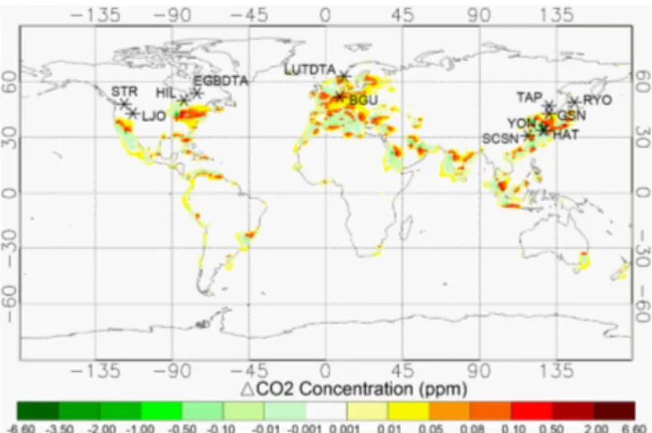
con-trol and experiment simulations offers additional insight into the impact of the regridding and coastal shuffling (Fig. 4). Similar to the emissions difference, the simulated CO2
con-centrations in the lowest model layer show differences along coastlines where large urban centers or point sources are present. In contrast to the emission differences, the response of surface CO2concentration reflects not only the
immedi-ate local emission impact but also a downwind impact as the differing concentration fields are transported by atmospheric motion. A particularly notable example is the surface CO2
Figure 4.Simulated PCTM surface annual mean surface CO2
con-centration difference (experiment minus control, units: ppm). The∗ in the figure denotes existing CO2monitoring locations where the
annual mean CO2concentration difference exceeds 2 ppm.
differences along the coastline driven by the emission dipole explained in Sect. 3.1, with negative values over ocean grid cells and positive values over the adjacent land grid cells.
The annual mean concentration differences range from −6.60 to +6.54 ppm at the grid cell scale. These CO2
concentration differences should be placed in the context of well-known surface concentration gradients such as the north–south gradient in annual mean CO2 concentration
of ∼4.0 ppm and Northern Hemisphere longitudinal gradi-ents of ∼1.5 ppm (Conway and Tans, 1999). These differ-ences represent a potential bias in the simulated CO2signal
at, or downwind from, numerous locations associated with coastal/urban areas, and are the combined result of the differ-ing emission distribution in the two experiments acted upon by the atmospheric transport.
3.3 Hourly CO2concentration
Here we examine the simulated CO2 concentration
differ-ences at locations where CO2 concentrations are directly
monitored, in an attempt to provide more guidance to at-mospheric CO2inversion studies that use these locations as
the observational constraint to estimating carbon exchange between the ocean, land and atmosphere. An examination of the hourly time series of CO2 concentration in the
low-est model layer at GLOBALVIEW monitoring stations in-dicates that 169 stations (out of 313 total GLOBALVIEW stations) show hourly CO2concentration differences greater
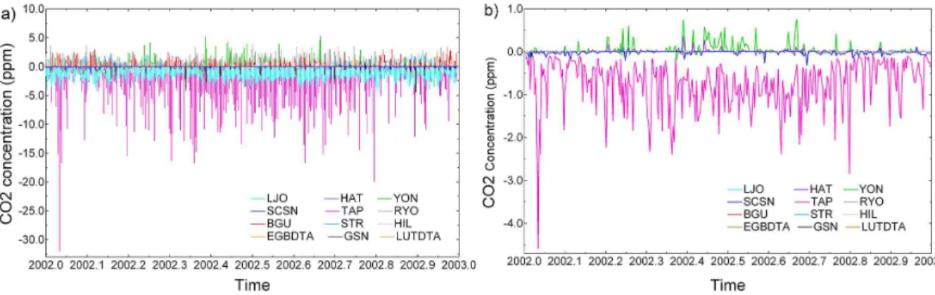
than ±0.10 ppm, and 12 of these stations show differences that exceed±2.0 ppm (Fig. 5). Most of the larger differences are located close to coastal urban areas and occur at night and the early morning hours. This is not surprising given the re-duction in mixing between the free troposphere and the plan-etary boundary layer at these times.
The hourly differences at these 12 stations range from −32.1 to +2.50 ppm. Tae-ahn Peninsula (TAP) has the largest response (−32.1 ppm). Yonagunijima (YON) and Gosan (GSN) also show large responses, with maximum dif-ferences reaching+5.23 and−4.43 ppm, respectively.
Given the fact that many atmospheric CO2inversions
sam-ple the simulated and observed CO2concentration as a
lo-cal afternoon average, and the simulated maximum differ-ences found here occur at varying times of day, greater in-sight can be gained by examining the simulated differences during the afternoon. In this case, 38 surface stations show hourly CO2concentration differences exceeding a magnitude
of±0.10 ppm during the local afternoon hours from 12:00 to 18:00 (hereafter referred as “local after noon mean”). Of the 38 stations, 5 (TAP, GSN, SCSN, YON and RYO) have a local afternoon mean difference ranging between 0.12 and −4.58 ppm (Fig. 5).
The shift between a positive and negative bias shown in Fig. 5 is owed to the fact that these coastal sites likely ex-perience onshore and offshore airflow at different times, and this changes which portion of the local emission dipole in-fluences the monitoring location. The specific circumstances at the TAP station are a good example of how the transport acts upon the emission dipoles to either enhance or diminish the concentration differences seen in Fig. 6. TAP is a coastal station (36◦43′N, 126◦07′E) located in the Tae-ahn Penin-sula (Republic of Korea). This site is in close proximity to the two cities of Seosan and Taean. TAP is assigned to an ocean grid cell on the PCTM grid. The emissions on this grid cell are aggregated to adjacent land grid cells after shuf-fling process. The site is thus located in the negative portion of the emission dipole (emission difference:−24.1 TgC grid cell−1yr−1) corresponding to the positive emission portion
on adjacent land grid cells, as displayed in Fig. 6a. Consis-tently, the TAP site lies in the negative portion of the annual mean surface CO2 concentration field (−6.60 ppm)
oppos-ing to the positive portion on land (Fig. 6b). Time series of the hourly concentration difference for the TAP site shows the largest value of about−32.1 ppm occurring on 13 Jan-uary at 5:00 p.m. local time. PCTM wind fields show low wind speeds on 12 January (daily mean: < 2 m s−1) and in the daytime of 13 January (3.5 m s−1) compared to the much higher monthly mean value (8.4 m s−1). The weak transport during this time period accentuates the difference between the two experiments by lessening the amount of horizontal mixing and dispersion of the dipole gradient in this location. The hourly time series for the TAP site also shows high-frequency behavior throughout the year, indicating the im-pact of synoptic-scale atmospheric transport. Another feature to note is the seasonal pattern in the hourly CO2
Figure 5.Simulated PCTM surface CO2concentration difference (experiment minus control, units: ppm) at the 12 GLOBALVIEW mon-itoring stations with the largest concentration difference. (a)Hourly mean CO2concentration difference;(b)local afternoon mean CO2
concentration difference.
Figure 6.Regional fluxes difference and simulated surface CO2concentration differences (experiment minus control) and the location of
GLOBALVIEW monitoring site TAP.(a)Flux difference;(b)concentration difference. Stars mark the location of the TAP site.
of the hourly time series also shows diurnal patterns in all 12 monitoring sites.
3.4 Implications for carbon cycle studies
Research in which simulated CO2 concentrations are
com-pared to observed must consider ways to avoid the poten-tial bias introduced when regridding high-resolution fossil fuel CO2emissions to the lower-resolution grids typical of
atmospheric transport models. Atmospheric CO2 inversion
studies are also a good example of research that must over-come this potential problem. However, we do not consider the impact and uncertainty on atmospheric inversion in this study, since atmospheric inversions are not the only purpose for simulations of fossil-fuel-like tracers. Many studies in at-mospheric chemistry have the same need and consequently the same problem. But the study also does do something of direct use for an inversion. The fossil fuel is part of the prior flux. So in an atmospheric inversion this term represents a systematic uncertainty in the mapping of fossil fuel flux into the prior mismatches (prior simulation of concentration – ob-servations). It can be seen that the effect is widespread and
large compared to the measurement uncertainty usually used. Thus, this is enough to demonstrate significance for an inver-sion.
Utilizing the shuffling procedure outlined here is one way to minimize this potential bias in the spatial distribution of the fossil fuel CO2 emissions. The goal is to maintain the
localization of the large emission gradients that occur near coastlines due to the preponderance of large cities and point sources while simultaneously ensuring dynamic consistency between the emissions and modeled atmospheric transport.
Alternatively, modelers could use data selection proce-dures to minimize potential bias when choosing which CO2
concentration observing sites to compare to simulated re-sults (e.g., Law, 1996). Some inversion model systems such as NOAA’s CarbonTracker model sample only the after-noon daytime measurements at quasi-continuous stations to avoid times when the model boundary layer is less reliable (e.g., nighttime) (Peters, et al., 2007). Eliminating or de-emphasizing (via the assignment of large uncertainty) atmo-spheric CO2monitoring locations that are near, or strongly
influenced by, large fossil fuel CO2sources can reduce the
given that many global carbon cycle studies are observation-ally underconstrained, this choice does come with potentiobservation-ally large information loss. Given this fact, we recommend the use of an emissions shuffling procedure.
It also should be pointed out that the fossil fuel emis-sions from planes and ships are not included in this study. Airborne emissions are unlikely to be strongly impacted by this problem since the differences in atmospheric physics between land and ocean decrease once above the boundary layer. While emissions from shipping do potentially suffer from this problem, the fraction subject to misallocation will be small so the total problem is a small fraction of a small fraction.
Many earth system models avail of “tiling” techniques which can assign more than one surface characteristic to a grid cell. It should be noted that the reshuffling simply might transfer errors from one place to another. For example reshuf-fling emissions away from an oceanic grid point may leave a station in that grid cell further from emissions than it re-ally should be. This is possible of course. This can only been investigated by separating the transport and relocation effects by using an online model. However, it is expected that this shuffling method could introduce land–ocean biases, since fixed fossil sources are almost entirely land-based and putting them in ocean grid points seems far more likely to in-troduce land–ocean biases as the inversion tries to correct a poorly transported signal from the wrong environment. Gen-erally, without further research testing the sensitivity of re-sults to this technique, it is unclear to what extent this mini-mizes the fossil fuel CO2emissions regridding problem
dis-cussed in this study.
4 Conclusions
This study tests the sensitivity of simulated CO2
con-centration to regridding of fossil fuel CO2 emissions
from a high-resolution grid to a coarser global atmo-spheric transport model grid. Two experiments are con-ducted. The first regrids from the fine to coarse grid but with no post-regridding adjustment to those emitting grid cells that inevitably ends up in the ocean (“con-trol”). The second experiment performs the same regrid-ding process as the first but moves or “shuffles” the ocean-based emissions to adjacent land grid cells in a propor-tional manner. The two experiments exhibit large fossil fuel CO2 emissions differences in coastal regions, which range
from −30.3 TgC grid cell−1yr−1 (−3.39 kgC m−2yr−1) to
+30.0 TgC grid cell−1yr−1 (+2.6 kgC m−2yr−1) which, when summed globally, are equivalent to 10 % of the 2002 global total fossil fuel CO2 emissions. After transport of
these emissions through a global tracer transport model, these two experiments show simulated CO2 concentration
differences along the coastal margin in both the spatial and temporal domains. The resulting annual mean surface
CO2 concentration difference when examining all surface
grid cells varies between −6.60 and +6.54 ppm. At the hourly level, individual CO2 concentration differences
ex-ceed±0.10 ppm at 38 monitoring stations, with a maximum of−32.1 ppm at 1 monitoring location. When examining lo-cal afternoon mean values, which both modeling systems and monitoring protocols emphasize, the CO2concentration
dif-ferences are as large as−4.58 ppm. These CO2 concentra-tion differences result from the shifted emissions acted upon by modeled meteorology and can result in biased flux esti-mation in atmospheric CO2 inversions which rely on
com-parison of simulated to measured CO2. This phenomenon is
also potentially important in any study investigating source– receptor simulations such as those found in air quality and other trace gas research efforts.
Code availability
The Fortran code to regrid and reallocate the surface fossil fuel emissions flux to ensure the dynamical consistence be-tween emission and global transport model is available from the correspondence author ([email protected]).
Acknowledgements. This work was supported by NASA CMS grant NNX12AP52G. P. Rayner is in receipt of an Australian Professorial Fellowship (DP1096309).
Edited by: G. Munhoven
References
Asefi-Najafabady, S., Rayner, P. J., Gurney, K. R., McRobert, A., Song, Y., Coltin, K., Huang, J., Elvidge, C., Baugh, K.: A multiyear, global gridded fossil fuel CO2 emission data
product: Evaluation and analysis of results, J. Geophys. Res., doi:10.1002/2013JD021296, 2014.
Bosilovich, M. G.: Regional climate and variability of NASA MERRA and recent reanalyses: U.S. summertime precipitation and temperature, J. Appl. Meteorol. Clim., 52, 1939–1951, 2013. Ciais, P., Paris, J.-D., Marland, G., Peylin, P. , Piao, S. L., Levin, I., Pregger, T., Scholz, Y., Friedrich, R., Rivier, L., Houwelling, S., Schulze, E. D. and members of the CARBOEUROPE Syn-thesis Team (1): The European carbon balance revisited. Part 4: fos sil fuel emissions, Glob. Change Biol., 16, 1395–1408, doi:10.1111/j.1365-2486.2009.02098.x, 2010.
Conway, T. J. and Tans P. P.: Development of the CO2latitude gra-dient in recent decades, Global Biogeochem. Cy., 13, 821–826, 1999.
Elvidge, C. D., Ziskin, D., Baugh, K. E., Tuttle, B. T., Ghosh, T., Pack, D. W., Erwin, E. H., and Zhizhin, M.: A Fifteen Year Record of Global Natural Gas Flaring Derived from Satellite Data, Energies, 2, 595–622, 2009.
Enting, I.: Inverse Problems in Atmospheric Constituent Transport, Cambridge Univ. Press, New York, 2002.
I. Y., Gloor, M., Heimann, M., Higuchi, K., John, J., Maki, T., Maksyutov, S., Masarie, K., Peylin, P., Prather, M., Pak, B. C., Randerson, J., Sarmiento, J., Taguchi, S., Takahashi, T., and Yuen, C.: Towards robust regional estimates of CO2sources and
sinks using atmospheric transport models, Nature, 415, 626–630, 2002.
Gurney, K. R., Chen, Y., Maki, T., Kawa, S. R., Andrews, A., and Zhu, Z.: Sensitivity of atmospheric CO2inversions to seasonal
and interannual variations in fossil fuel emissions, J. Geophys. Res., 110, d10308, doi:10.1029/2004JD005373, 2005.
Kawa, S. R., Erickson III, D. J., Pawson, S., and Zhu, Z.: Global CO2 transport simulations using meteorological data from the
NASA data assimilation system, J. Geophys. Res., 109, D18312, doi:10.1029/2004JD004554, 2004.
Kawa, S. R., Mao, J., Abshire, J. B., Collatz, G., J., and Weaver, C. J.: Simulation studies for a space-based CO2lidar, Tellus, 62B,
759–769, 2010.
Law, R.: The selection of model-generated data CO2data: a case
study with seasonal biospheric sources, Tellus, 48B, 474–486, 1996.
Le Quéré, C., Andres, R. J., Boden, T., Conway, T., Houghton, R. A., House, J. I., Marland, G., Peters, G. P., van der Werf, G. R., Ahlström, A., Andrew, R. M., Bopp, L., Canadell, J. G., Ciais, P., Doney, S. C., Enright, C., Friedlingstein, P., Huntingford, C., Jain, A. K., Jourdain, C., Kato, E., Keeling, R. F., Klein Gold-ewijk, K., Levis, S., Levy, P., Lomas, M., Poulter, B., Raupach, M. R., Schwinger, J., Sitch, S., Stocker, B. D., Viovy, N., Zaehle, S., and Zeng, N.: The global carbon budget 1959–2011, Earth Syst. Sci. Data, 5, 165–185, doi:10.5194/essd-5-165-2013, 2013. Masarie, K. A. and Tans, P. P.: Extension and Integration of Atmo-spheric Carbon Dioxide Data into a Globally Consistent Mea-surement Record, J. Geophys. Res., 100, 11593–11610, 1995. Lock, A. P., Brown, A. R., Bush, M. R., Martin, G. M., and Smith,
R. N. B.: A new boundary layer mixing scheme. Part I: Scheme description and single-column model tests, Mon. Weather Rev., 138, 3187–3199, 2000.
Louis, J., Tiedtke, M., and Geleyn, J.: A short history of the PBL parameterization at ECMWF. Proc. ECMWF Workshop on Plan-etary Boundary Layer Parameterization, Reading, UK, ECMWF, 59–80, 1982.
McGrath-Spangler, E. L. and Molod, A.: Comparison of GEOS-5 AGCM planetary boundary layer depths computed with various definitions, Atmos. Chem. Phys., 14, 6717–6727, doi:10.5194/acp-14-6717-2014, 2014.
Nassar, R., Napier-Linton, L., Gurney, K. R., Andres, R. J., Oda, T., Vogel, F. R., and Deng, F.: Improving the temporal and spatial distribution of CO2 emissions from global fossil fuel emission
data sets, J. Geophys. Res.-Atmos., 118, 917–933, 2013.
Oda, T. and Maksyutov, S.: A very high-resolution (1 km×1 km) global fossil fuel CO2emission inventory derived using a point
source database and satellite observations of nighttime lights, At-mos. Chem. Phys., 11, 543–556, doi:10.5194/acp-11-543-2011, 2011.
Peters, W., Jacobson, A. R., Sweeney, C., Andrews, A. E., Conway, T. J., Masarle, K., Miller, J. B., Bruhwiler, L. M. P., P˙etron, G., Hirsch, A. I., Worthy, D. E. J., vander Werf, G. R., Randerson, J. T., Wennberg, P. O., Krol, M. C., and Tans, P. P.: An atmospheric perspective on North American carbon dioxide exchange: Car-bonTracker, P. Natl. Acad. Sci. USA, 104, 18925–18930, 2007. Peylin, P., Houweling, S., Krol, M. C., Karstens, U., Rödenbeck, C.,
Geels, C., Vermeulen, A., Badawy, B., Aulagnier, C., Pregger, T., Delage, F., Pieterse, G., Ciais, P., and Heimann, M.: Importance of fossil fuel emission uncertainties over Europe for CO2
mod-eling: model intercomparison, Atmos. Chem. Phys., 11, 6607– 6622, doi:10.5194/acp-11-6607-2011, 2011.
Rayner, P. J., Raupach, M. R., Paget, M., Peylin, P., and Koffi, E.: A new global gridded data set of CO2emissions from fossil fuel combustion: Methodology and evaluation, J. Geophys. Res., 115, D19306, doi:10.1029/2009JD013439, 2010.
Reichle, R. H.: The MERRA-Land Data Product, version 1.1. GMAO Technical Report, NASA Global Modeling and Assim-ilation Office, Goddard Space Flight Center, Greenbelt, MD, USA, available at: http://gmao.gsfc.nasa.gov/merra/ (last access: 30 November 2014), 2012.
Reichle, R. H., Koster, R. D., De Lannoy, G. J. M., Forman, B. A., Liu, Q., Mahanama, S. P. P., and Toure, A.: Assessment and enhancement of MERRA land surface hydrology estimates, J. Climate, 24, 6322–6338, doi:10.1175/JCLI-D-10-05033.1, 2011. Rienecker, M. M., Suarez, M. J., Gelaro, R., Todling, R., Bacmeis-ter, J., Liu, E., Bosilovich, M. G., Schubert, S. D., Takacs, L., Kim, G.-K., Bloom, S., Chen, J., Collins, D., Conaty, A., Silva, A. D., Gu, W., Joiner, J., Koster, R. D., Lucchesi, R., Molod, A., Owens, T., Pawson, S., Pregion, P., Redder, C. R., Reichle, R., Robertson, F. R., Ruddick, A. G., Sienkiewicz, M., and Woollen, J.: MERRA – NASA’s Modern-Era Retrospective Analysis for Research and Applications, J. Climate, 24, 3624– 3648, doi:10.1175/JCLI-D-11-00015.1, 2011.
Wang, R., Tao, S., Ciais, P., Shen, H. Z., Huang, Y., Chen, H., Shen, G. F., Wang, B., Li, W., Zhang, Y. Y., Lu, Y., Zhu, D., Chen, Y. C., Liu, X. P., Wang, W. T., Wang, X. L., Liu, W. X., Li, B. G., and Piao, S. L.: High-resolution mapping of combustion processes and implications for CO2emissions, Atmos. Chem. Phys., 13,