Long-term dynamics of OH * temperatures over central Europe: trends and solar correlations

www.atmos-chem-phys.net/16/15033/2016/ doi:10.5194/acp-16-15033-2016

© Author(s) 2016. CC Attribution 3.0 License.

Long-term dynamics of OH

∗

_{temperatures over central Europe:}

trends and solar correlations

Christoph Kalicinsky1, Peter Knieling1, Ralf Koppmann1, Dirk Offermann1, Wolfgang Steinbrecht2, and Johannes Wintel1

1_{Institute for Atmospheric and Enviromental Research, University of Wuppertal, Wuppertal, Germany} 2_{DWD, Hohenpeissenberg Observatory, Germany}

Correspondence to:Christoph Kalicinsky (kalicins@uni-wuppertal.de)

Received: 6 April 2016 – Published in Atmos. Chem. Phys. Discuss.: 7 June 2016 Revised: 26 October 2016 – Accepted: 27 October 2016 – Published: 6 December 2016

Abstract. We present the analysis of annual average OH∗ temperatures in the mesopause region derived from measure-ments of the Ground-based Infrared P-branch Spectrometer (GRIPS) at Wuppertal (51◦N, 7◦E) in the time interval 1988 to 2015. The new study uses a temperature time series which is 7 years longer than that used for the latest analysis regard-ing the long-term dynamics. This additional observation time leads to a change in characterisation of the observed long-term dynamics.

We perform a multiple linear regression using the solar ra-dio flux F10.7 cm (11-year cycle of solar activity) and time to describe the temperature evolution. The analysis leads to a linear trend of (−0.089±0.055) K year−1 _{and a} sensitiv-ity to the solar activsensitiv-ity of (4.2±0.9) K(100 SFU)−1_(r2_of fit 0.6). However, one linear trend in combination with the 11-year solar cycle is not sufficient to explain all observed long-term dynamics. In fact, we find a clear trend break in the temperature time series in the middle of 2008. Before this break point there is an explicit negative linear trend of (−0.24±0.07) K year−1, and after 2008 the linear trend turns positive with a value of (0.64±0.33) K year−1. This ap-parent trend break can also be described using a long periodic oscillation. One possibility is to use the 22-year solar cycle that describes the reversal of the solar magnetic field (Hale cycle). A multiple linear regression using the solar radio flux and the solar polar magnetic field as parameters leads to the regression coefficients Csolar=(5.0±0.7) K(100 SFU)−1 andChale=(1.8±0.5)K(100 µT)−1(r2=0.71). The sec-ond way of describing the OH∗ temperature time series is to use the solar radio flux and an oscillation. A least-square fit leads to a sensitivity to the solar activity of

(4.1±0.8) K(100 SFU)−1, a period P=(24.8±3.3) years, and an amplitude Csin=(1.95±0.44) K of the oscillation (r2=0.78). The most important finding here is that using this description an additional linear trend is no longer needed. Moreover, with the knowledge of this 25-year oscillation the linear trends derived in this and in a former study of the Wup-pertal data series can be reproduced by just fitting a line to the corresponding part (time interval) of the oscillation. This ac-tually means that, depending on the analysed time interval, completely different linear trends with respect to magnitude and sign can be observed. This fact is of essential impor-tance for any comparison between different observations and model simulations.

1 Introduction

to months in the case of planetary waves (e.g. Bittner et al., 2000; Offermann et al., 2009; Perminov et al., 2014) and on the timescale of several minutes in the case of gravity waves (e.g. Offermann et al., 2011; Perminov et al., 2014). Beside these rather short-term fluctuations the temperature in the mesopause region also exhibits long-term variations on a timescale of several years. Although the amplitudes of these long-term variations are much smaller, the long-term change of the mesopause temperatures is, nevertheless, clearly exis-tent and important. Several previous studies showed the ex-istence of an 11-year modulation of the temperature in co-incidence with the 11-year cycle of solar activity which is visible in the number of sunspots and the solar radio flux F10.7 cm (for a review of solar influence on mesopause tem-perature see Beig, 2011a). The reported sensitivities in the middle to high latitudes of the Northern Hemisphere lie between 1 to 6 K(100 SFU)−1_{. Another type of long-term} change is linear trends in the analysed time interval. In the mesopause region of the Northern Hemisphere such trends range from about zero up to a cooling of 3 K decade−1 (for a review of mesopause temperature trends see Beig, 2011b). Trend breaks also seem to be possible where the linear trend switches its sign (positive or negative trend) or the magnitude of the trend significantly changes (for an example of the lat-ter case see Offermann et al., 2010). In cases of such changes in trend (e.g. caused due to changes in trend drivers) a piece-wise linear trend approach can be used, in which different linear trends are determined for different time intervals (e.g. Lastovicka et al., 2012).

Beside these variations of the mesopause temperature, Höppner and Bittner (2007) found a quasi 22-year modula-tion of the planetary wave activity which they derived from mesopause temperature measurements. This observed mod-ulation coincides with the reversal of the solar polar netic field, the so-called Hale cycle. The solar polar mag-netic field reverses every approximately 11 years at about solar maximum, thus the maximum positive and negative values of magnetic field strength occur between two con-secutive solar maxima (e.g. Svalgaard et al., 2005). Several studies exist showing a quasi 22-year modulation of different meteorological parameters such as temperature, rainfall, and temperature variability that are in phase with the Hale cycle or the double sunspot cycle (e.g. Willet, 1974; King et al., 1974; King, 1975; Qu et al., 2012), but no physical mech-anism is found for these coincidences. The double sunspot cycle is another type of Hale cycle with a period of about 22 years which is phase-shifted compared to the Hale cycle of the solar polar magnetic field. The maxima and minima of the double sunspot cycle occur at maxima of the sunspot number (e.g. King, 1975; Qu et al., 2012). However, a num-ber of possible influences, also showing a 22-year modula-tion, are named: galactic cosmic rays (GCR), solar irradia-tion, and solar wind (e.g. White et al., 1997; Zieger and Mur-sula, 1998; Scafetta and West, 2005; Miyahara et al., 2008; Thomas et al., 2013; Mursula and Zieger, 2001).

Because of this large number of influences and possible interactions the analysis of the temperatures is not easy to in-terpret, but due to the different timescales of the variations the different types of influences and phenomena can some-times be distinguished. In this paper we focus on the long-term variations of the mesopause temperature on timescales larger than 10 years. We use OH∗temperatures, which have been derived from ground-based measurements of infrared emissions at a station in Wuppertal (Germany), for our anal-yses.

The paper is structured as follows. In Sect. 2 we describe the instrument and measurement technique and show the OH∗temperature observations, Sect. 3 introduces the Lomb– Scargle periodogram and its properties, and in Sect. 4 we analyse the OH∗ _{temperatures regarding solar correlations,}

long-term trends, and long periodic oscillations. A discussion of the obtained results is given in Sect. 5, and we summarise and conclude in Sect. 6.

2 Observations

2.1 Instrument and measurements

Excited hydroxyl (OH∗) molecules in the upper meso-sphere/mesopause region emit radiation in the visible and near infrared. The emission layer is located at about 87 km height with a layer thickness of approximately 9 km (full width at half maximum) (e.g. Baker and Stair Jr., 1998; Ober-heide et al., 2006). The GRIPS-II (Ground-based Infrared P-branch Spectrometer) instrument is a Czerny–Turner spec-trometer with a Ge detector cooled by liquid nitrogen. It mea-sures the emissions of the P1(2), P1(3), and P1(4) lines of the OH∗(3,1) band in the near infrared (1.524–1.543 µm) (for ex-tensive instrument description see Bittner et al., 2000, 2002). The measurements are taken from Wuppertal (51◦N, 7◦E) every night with a time resolution of about 2 min. Thus, a continuous data series throughout the year is obtained with data gaps caused by cloudy conditions only. This results in approximately 220 nights of measurements per year (Ober-heide et al., 2006; Offermann et al., 2010). The relative in-tensities of the three lines are used to derive rotational tem-peratures in the region of the OH∗emission layer (see Bittner et al., 2000, and references therein).

spectrom-160

180

200

220

240

Nightly avg. temp. [K]

1990

1995

_{Time [years]}

2000

2005

2010

2015

192

196

200

204

208

T

[K

]

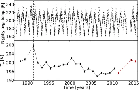
Figure 1.OH∗temperature time series derived from GRIPS-II and GRIPS-N measurements at Wuppertal. The upper panel shows the nightly

average temperatures and the lower panel shows the annual average temperaturesT0. EachT0is plotted in the middle of the corresponding

year and the dates given at thexaxis show the beginning of the years. The annual average temperatures partly or completely derived from

the new instrument between 2011 and 2015 are shown in red in the lower panel. The error bars show the estimated 1σuncertaintiesσT0 of

the temperaturesT0(based on the standard deviation of the residuals). The vertical dashed line marks the date of Mt Pinatubo eruption.

eter, equipped with a thermoelectrically cooled InGaAs de-tector. The optical and spectral properties of GRIPS-N and GRIPS-II are very similar, thus the measurements of both in-struments are nearly identical. The new GRIPS-N instrument was operated without further problems since the beginning of 2014. Hence, for the years 2014 and 2015 a complete set of measurements is available with only the typical data gaps due to cloudiness.

2.2 Data processing

The nightly average OH∗ temperatures derived from the GRIPS-II and GRIPS-N measurements in Wuppertal are shown in the upper panel of Fig. 1 for the time interval 1988 to 2015. As mentioned above the data series show larger gaps of several months due to technical problems in the years 2012 and 2013 and, additionally, a data gap of 3 months at the be-ginning of 1990. These years have to be excluded from the analysis, since a reasonable determination of an annual aver-age temperature in the presence of such large data gaps is not possible.

By far the largest variation in this temperature series is the variation over the course of a year. In order to evalu-ate the data with respect to long-term dynamics with peri-ods well above 1 year the seasonal variation has to be elim-inated first. Since the temperature series exhibits data gaps mostly due to cloudy conditions, a simple arithmetic mean for each year is not advisable. We follow the method used be-fore in several analyses (e.g. Bittner et al., 2002; Offermann et al., 2004, 2006, 2010; Perminov et al., 2014) and perform a harmonic analysis based on least-square fits for each year

separately. As described in Bittner et al. (2000) the seasonal variation is characterised by an annual, a semi-annual, and a ter-annual cycle. Thus, the temperature variation over 1 year is described by

T =T0+ 3

X

i=1 Ai·sin

2·π·i 365.25(t+φi)

, (1)

whereT0is the annual average temperature,t is the time in days of the year, andAi,φi are the amplitudes and phases of the sinusoids. By fitting this equation to the temperature data we can obtain the best possible estimate of the annual aver-age temperatureT0for each year. A year in this case denotes a calendar year. The resulting annual average temperatures are shown in the lower panel of Fig. 1 with data gaps in the years 1990, 2012, and 2013 (illustrated by the dashed lines). The seasonal variation of the year 2009 is shown in Fig. 2 as a typical example. As described above a detector failure in mid-2011 stopped the GRIPS-II measurements. The follow-ing measurements were performed with a new instrument. The first year of full data coverage with GRIPS-N was 2014. Due to this the correspondingT0for 2011 and 2014–2015 are marked in red in Fig. 1.

2.3 Comparison with other observations

0 50 100 150 200 250 300 350 DOY

150 160 170 180 190 200 210 220 230 240

Temperature [K]

Figure 2.GRIPS-II nightly average temperatures of 2009 plotted at the day of year (DOY). The measurement data are shown in black and the harmonic fit using Eq. (1) is shown as the red curve.

2004

2006

2008

_{Time [years]}

2010

2012

2014

2016

192

194

196

198

200

202

204

T

[K

]

GRIPS WUP GRIPS HPB

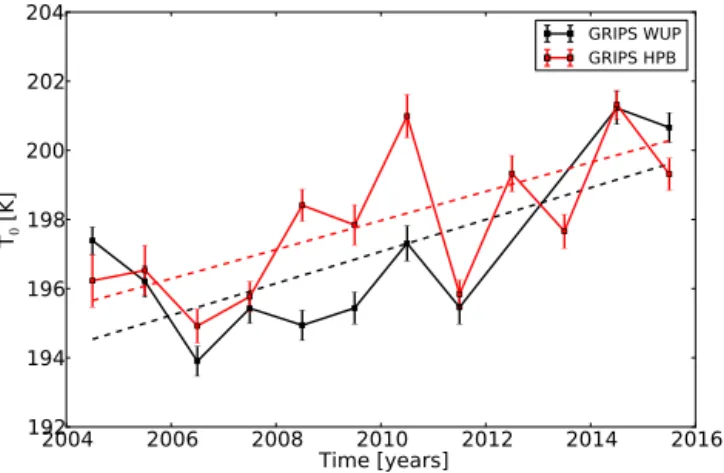
Figure 3. OH∗ annual average temperatures for the two stations Wuppertal and Hohenpeissenberg in the time interval 2004–2015. The temperatures for Wuppertal (WUP) are shown in black and the temperatures for Hohenpeissenberg (HPB) in red. The dashed lines show the linear fits to the corresponding time series. The linear fit for the Hohenpeissenberg time series only considers measurements at times Wuppertal measurements are also available.

We compare the Wuppertal observations with observations of OH∗ temperatures taken from Hohenpeissenberg (48◦N, 11◦E) to check this. The instrument GRIPS-I in Hohenpeis-senberg measures in the same spectral range and uses the same data processing technique to determine OH∗

tempera-tures. GRIPS-I is an Ebert–Fastie spectrometer with a liquid-nitrogen-cooled Ge detector (see e.g. Bittner et al., 2002). The measurements at Hohenpeissenberg started end of 2003. Figure 3 shows the comparison for the two measurement stations. A significant correlation between the two time se-ries can be found with a correlation coefficientr=0.72. The comparably low value ofr is caused by the differences be-tween 2007 to 2009, where the temperatures at Wuppertal partly decrease (increase) and the Hohenpeissenberg

tem-peratures increase (decrease) at the same time. These dif-ferences are most likely caused by local effects. Further-more, the largest absolute difference in 2010 is caused by an exceptional warm summer observed at Hohenpeissenberg. This warm summer is also observed at the nearby station in Oberpfaffenhofen (see Schmidt et al., 2013, their Fig. 12.) but not at Wuppertal.

The linear increase for each time series is shown in Fig. 3 as dashed lines in black and red. In order to get the most appropriate comparison the linear fit to the Ho-henpeissenberg time series only considers data points at times where measurements at Wuppertal are also available. The linear increase during the last 12 years at Wuppertal is (0.46±0.17) K year−1and the increase at Hohenpeissenberg is (0.42±0.16) K year−1_{. Both values agree very well, but} the two lines are shifted towards each other indicating an off-set between the two stations. This offoff-set is about 0.9 K with Hohenpeissenberg being warmer. In a former study Offer-mann et al. (2010) obtained a mean offset between the two stations of 0.8 K for the time interval 2004–2008. Thus, this comparison agrees well the former study. Offermann et al. (2010) suggested that the latitudinal difference between the stations is responsible for this small difference. The tempera-ture differences between the minima in 2006 and the maxima in 2014 also agree very well for both stations. The values are (7.3±0.7) K at Wuppertal and (6.4±0.7) K at Hohenpeis-senberg. Since we analysed the relative evolution of the tem-perature series at Wuppertal, the last data points were found to fit the whole picture of the long-term development of OH∗_{temperatures. Thus, the temperature increase observed}

at Wuppertal in recent years is reliable and confirmed by the temperature increase observed at Hohenpeissenberg.

The latest analysis of the OH∗_{temperatures at Wuppertal}

regarding long-term dynamics was performed for the time in-terval 1988–2008 (Offermann et al., 2010). The current study now considers a time series which is 7 years longer than that used before. The clear temperature increase over the last years has encouraged us to perform a new analysis regarding the long-term dynamics.

3 Lomb–Scargle periodogram and false alarm probability

algorithm by Townsend (2010) for the fast calculation of the periodogram.

An important quantity for the interpretation of a LSP is the so called false alarm probability (FAP). The FAP gives the probability that a peak of height zin the periodogram is caused just by chance, e.g. by noise. As already pointed out by Scargle (1982), the cumulative distribution function (CDF) can be used to determine the FAP. If we take dif-ferent samples of noise, calculate the LSP for each sample and then determine the heightzof the maximum peak, the CDF of all these heights z gives the probability that there is a heightZ smaller or equal toz. Consequently, the value 1−CDF gives the probability that there is a heightZlarger thanzby chance. Thus, 1−CDF gives the FAP. Another im-portant point in this context is the normalisation of the pe-riodogram, since the normalisation affects the type of distri-bution of the periodogram, thus the description of the FAP (for a more detailed discussion see e.g. Horne et al., 1986; Schwarzenberg-Czerny, 1998; Cumming et al., 1999; Zech-meister and Kürster, 2009). We use the normalisation by the total variance of the data, which leads to a beta distribution in the case of Gaussian noise (Schwarzenberg-Czerny, 1998). Since a mean has to be subtracted from the data before calcu-lating the LSP, the total variance is determined usingN−1 degrees of freedom withNbeing the number of data points. This leads to a maximum value for a peak in the periodogram of(N−1)/2 in the case of a single sinusoid. The FAP can be described by

FAP=1−

"

1−

2z N−1

(N−3)/2#Ni

, (2)

whereN is the number of data points andNi is the number of independent frequencies (Schwarzenberg-Czerny, 1998; Cumming et al., 1999; Zechmeister and Kürster, 2009). The number of independent frequenciesNi has to be determined using simulations, since it is not possible to easily describe this quantity analytically (Cumming et al., 1999). It depends on several factors, e.g. the number of data pointsN and the spacing of the data points. Horne et al. (1986) showed the partly large effect of the spacing (randomly or clumps of points) onNi. Therefore, we perform simulations to deter-mineNifor the special situation of our observations. We take random values from a Gaussian distribution and the spacing of our observations as input. Then we calculate the LSP for ten thousand such noise samples in the same way as for the real data and determine the heightzof the maximum peak for each LSP. Every LSP is evaluated in the frequency range from Nyquist-frequencyf =1/2 year−1tof =1/Tyear−1, whereT in our case is 35 years, since we want to search for periodicities in range of the time window of the data series of 28 years. Periodicities in this range are surely accompa-nied with larger uncertainties, but the LSP gives a reasonable overview over the periodicities, even the large ones, included in the time series. The LSP is calculated at 4Tdur1f=53

0.0 0.2 0.4 0.6 0.8 1.0

Pr

ob

(Z

z

)

2 3 4 5 6 7 8

Peak height z 10-3

10-2 10-1 100

Pr

ob

(Z

>

z

)

Simulations Theoretical fit

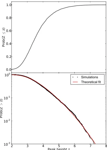
Figure 4.Distribution for peak heightszdetermined using random values from a Gaussian distribution as input for the calculation of LSP (for details see Sect. 3). The upper panel shows the

empiri-cal CDF, thus, the probability that there is a heightZ smaller or

equal toz. The FAP (probability that a heightZ larger zoccurs

just by chance) is shown in the lower panel. The simulation results are shown in black and a fit to the theoretical curve from Eq. (2) is

shown in red. Note the logarithmic scale of theyaxis of the lower

panel. This calculations are done for a data sampling same as that of the time series from 1988 to 2015 including data gaps. The fit leads

to a number of independent frequenciesNi=32.4.

1990

1995

2000

2005

2010

2015

Time [years]

50

100

150

200

250

Solar radio flux F10.7 cm [SFU]

Figure 5.Monthly average values of the solar radio flux F10.7 cm. The red dots mark the annual average values corresponding to the times of the GRIPS data points. The data were provided by Natural Resources Canada, Space Weather Canada.

4 Analysis of long-term dynamics: linear trend, solar correlations, long periodic, and multi-annual oscillations

4.1 Linear trend and 11-year solar cycle

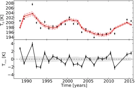
We analyse the long-term trend and the correlation with the 11-year cycle in solar activity by means of a multiple linear regression. For this and the following analyses the time coor-dinate is shifted such as the first data point (1988.5) is set to zero. The annual average temperatures are described by T0(t,SF)=Ctrend·t+Csolar·SF+b, (3) where Ctrend and Csolar are the two regression coeffi-cients, t is the time in years, b is a constant offset, and SF is the solar radio flux F10.7 cm in solar flux units (SFU). The solar radio flux is shown in Fig. 5 for the time interval from 1988 to 2015. The monthly av-erage values of the solar radio flux F10.7 cm were pro-vided by Natural Resources Canada (Space Weather Canada) and were obtained from http://www.spaceweather.gc.ca/ solarflux/sx-5-mavg-en.php. There are three solar max-ima in this time interval at about 1991, 2001, and 2014. This corresponds well to the annual average tempera-tures T0, which also show local maxima at these points. The calculated regression coefficients determined by fit-ting Eq. (3) using the method of ordinary least squares areCtrend=(−0.089±0.055)K year−1andCsolar=(4.2± 0.9)K(100 SFU)−1. Thep values (for the null hypothesis test) are 0.12 forCtrendand below 0.01 forCsolar. The 1σ un-certainties for the parameters given here (and in the follow-ing cases) are based on the standard deviation of the residuals to account for variations not captured by the fit. The whole fit has ar2=0.6. Figure 6 shows the results for this anal-ysis. The upper panel of the figure shows the temperature

time series in black and the fit according to Eq. (3) in red. Additionally, the residualTres is shown in the lower panel. Obviously, a fit taking into account a linear trend and the correlation with the 11-year solar cycle is a relatively poor fit to the temperature time series. When comparing the fit with the temperature time series, one has to additionally keep in mind that the general shape of the fit cannot change, since it depends on the time and solar flux values, which are fixed. The temperature residual still shows a temperature decrease until about 2005 and a temperature increase afterwards. In particular, the large increase at the end of the time series is not captured by the fit. Although there is an increase in solar activity in the same time interval, it is by far not enough to completely explain the observed temperature increase until 2015.

194

196

198

200

202

204

206

208

T

[K

]

1990

1995

_{Time [years]}

2000

2005

2010

2015

4

2

0

2

4

T

[K

]

Figure 6.The upper panel of the figure shows the time series of annual average OH∗temperatures in black and the fit corresponding to

Eq. (3) with the regression coefficientsCtrend=(0.089±0.055) K year−1andCsolar=(4.2±0.9) K(100 SFU)−1in red. The black error

bars show the uncertainties of the temperaturesσT0and the reddish area defined by the dashed red lines shows the 1σuncertaintyσfitof the

fit. In the lower panel the residualTresof the two is shown. The black error bars show the uncertainties of the temperaturesσT0 and the gray

area around the zero line shows the uncertainty of the fit.

0 5 10 15 20 25 30 35

Period [years] 0

1 2 3 4 5 6 7 8

Norm. power

Figure 7.The Lomb–Scargle periodogram for the time series of

an-nual OH∗temperatures (see Fig. 1 lower panel) is shown in black

and the LPS for the residual after subtracting the fit according to Eq. (3) (see Fig. 6 lower panel) is shown in red. The LSP is

evalu-ated at 53 evenly spaced frequencies in the rangef =1/2 year−1to

f =1/35 year−1. The dashed black horizontal lines display the

lev-els for false alarm probabilities of 0.01, 0.1, and 0.5 (top to bottom). The false alarm probabilities are calculated according to Eq. (2)

us-ingNi=32.4 and the number of data pointsN=25.

4.2 Trend break

The trend break and the correlation with the 11-year solar cycle are analysed by describing the annual average temper-atures as

T0(t,SF)=Csolar·SF+trend2phase(t ), (4)

where trend2phase(t )is a trend term using two lines to intro-duce the trend break. The trend term is written as

trend2phase(t )=

Ctrend1·t+b1 :t≤BP Ctrend2·t+b2 :t >BP

, (5)

where BP is the break point (in years). Since the two different lines need to be equal at the break point, this leads to the condition

Ctrend1·BP+b1=Ctrend2·BP+b2

⇔b2=b1+(Ctrend1−Ctrend2)·BP. (6) Thus, Eq. (5) can be rewritten as

trend2phase(t ) (7)

=

Ctrend1·t+b1 :t≤BP

Ctrend2·t+(b1+(Ctrend1−Ctrend2)·BP) :t >BP .

The description of the concept and the condition can be seen in Ryan and Porth (2007). Equation (4) now describes the annual average temperatures by using the correlation with the solar flux and a trend term with two different phases, where both phases have a linear temperature behaviour. These two phases are coupled by the variable break point BP.

1990 1995 2000 2005 2010 2015

Time [years]

6 4 2 0 2 4 6

Tre

s

[

K

]

200 150 100 50 0 50 100 150 200

Ma

gn

et

ic

fi

el

d [

µT

]

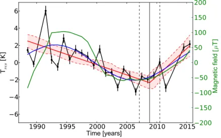
Figure 8.Residual for the temperature time series after removing the 11-year solar cycle (Csolar=(3.3±0.9) K(100 SFU)−1) and

subtract-ing the mean. The black error bars show the uncertaintiesσT0. The red lines show the fit according to Eq. (7) and the blue curve the fit

according to Eq. (8). The reddish area defined by the red dashed lines shows the 1σ uncertaintyσ_fitof the complete fit according to Eq. (7).

The break point BP is marked by the vertical black line and the corresponding uncertainties are shown as vertical dashed black lines. Addi-tionally, the annual average values of the solar polar magnetic field strength are displayed as a green curve with a second axis to the right.

Shown are the average values for the solar North Pole and South Pole with the magnetic field orientation of the North Pole ((N–S)/2). The

data were provided by the Wilcox Solar Observatory (for an instrument description see Scherrer et al., 1977).

break in the middle of 2008 (BP=(2008.8±1.7) year). Before the trend break in 2008 there is a negative tem-perature trend Ctrend1=(−0.24±0.07) K year−1 and af-ter the break point the trend is positive with a slope Ctrend2=(0.64±0.33) K year−1. The r2 of the whole fit is 0.74. The LSP for the residual after subtracting the trend break fit is shown in Fig. 9 in red. The former large peak at the right end of the periodogram for the original data series (black curve) is nearly completely removed after subtracting the trend break fit. Thus, the fit using two linear trends and a trend break explains a very large portion of the long-term variation of the OH∗temperature series.

4.3 Long-term oscillation

We analyse the possibility of an oscillation instead of a trend break. In order to get an idea about the oscillation we fit a sinusoid of the form

Tres(t )=A·sin

2·π P (t+φ)

+b (8)

to the temperature residual after subtracting the solar depen-dence and the mean (see Fig. 8 black curve).Adenotes the amplitude,P the period, and φthe phase. Additionally, we fit an offset b, since the mean of the temperature residual is not necessarily identical to the zero crossing of the os-cillation. The resulting oscillation is shown in Fig. 8 as a blue curve. The important estimated parameters of the fit are an amplitudeA=(2.06±0.43) K and a period of about 26 years (P=(26.3±3.2) years). It is clear that this oscilla-tion and the fit using the two linear phases and a trend break

0 5 10 15 20 25 30 35

Period [years] 0

1 2 3 4 5 6 7 8

Norm. power

Figure 9.The Lomb–Scargle periodogram for the time series of

annual OH∗temperatures (see Fig. 1 lower panel) is shown in black

and the LPS for the residual after subtracting the fit according to Eq. (4) is shown in red. For details see description of Fig. 7.

such a second trend break in the temperature series in the mid-1990s, about 1993.

Very prominent is the fact that the oscillation has a period of about 26 years with a minimum at about 2006 and a maxi-mum at about 1993. This type of oscillation with very similar parameters can be found on the sun. The original solar cycle (Hale cycle) is a cycle with a period of about 22 years and de-scribes the reversal of the magnetic field of the sun. The solar polar magnetic field of the sun is shown in Fig. 8 as a green curve with a second axis to the right. The solar polar field strength data were provided by the Wilcox Solar Observatory and were obtained from http://wso.stanford.edu/Polar.html. We used the low pass filtered values. Evidently, the oscilla-tion fitted to Tres and the Hale cycle of the magnetic field are very similar in the time interval shown. The correlation coefficient for a linear regression between the magnetic field and the temperature residual (black curve in Fig. 8) is r= 0.55. The corresponding slope is (1.74±0.56) K(100 µT)−1 (p value<0.01). This is a remarkable accordance between the observed oscillation in atmospheric temperature and so-lar poso-lar magnetic field.

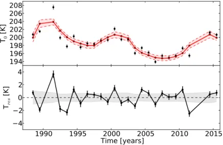
The long periodic oscillation describes the largest part of the temperature variability after detrending the temperature series with respect to the 11-year solar cycle. Thus, we anal-yse the temperature seriesT0by means of a multiple linear regression again to fit all dependencies simultaneously. We include the solar polar magnetic field in the equation, which replaces the linear trend. Hence, Eq. (3) transforms to T0(SF, Bsolar)=Csolar·SF+Chale·Bsolar+b, (9) whereBsolardenotes the solar polar magnetic field andChale the corresponding regression coefficient. The analysis leads to the results for the regression coefficients Csolar=(5.0± 0.7) K(100 SFU)−1 and Chale=(1.8±0.5) K(100 µT)−1. The fit to the temperature time series has ar2=0.71. This value is larger than the value for the fit including the 11-year solar cycle and one linear trend, which has ar2=0.6 (see Sect. 4.1), but it is slightly lower than ther2=0.74 of the trend break fit (see Sect. 4.2). An additional linear trend added to Eq. (9) does not significantly change the results. The obtained linear trend is insignificant in this case; therefore, it is excluded. The resulting fit and the residual are shown in Fig. 10. The fit curve (red colour) shows good agreement with the long-term variation of the temperature (black dots), but there are still some differences, especially at the begin-ning and the end of the time series. Additionally, the temper-ature residual (lower panel of Fig. 10) seems to show a long periodic oscillation. The LSP for the residual (red curve in Fig. 11) shows that the former large peak at the long periodic end of the periodogram (black curve) is largely reduced af-ter subtracting the fit, which shows that the description using the 11-year solar cycle and the Hale cycle explains most of the variance in the long periodic range. It is possible that an oscillation with similar parameters to the Hale cycle, which

are slightly changed (in amplitude, phase, and/or period), can describe the annual average temperatures even better.

We analyse this possibility and add an oscillation to the temperature description, which replaces the solar polar mag-netic field. Since the oscillation and the 11-year solar cycle are non-orthogonal functions, here we fit all dependencies simultaneously. The equation transforms to

T0(SF, t )=Csolar·SF+Csin·sin

2·π P (t+φ)

+b, (10) whereCsinis the amplitude,P is the period,φis the phase of the oscillation, andt is the time in years. The results of the least-square fit areCsolar=(4.1±0.8) K(100 SFU)−1for the sensitivity to the solar activity,Csin=(1.95±0.44) K for the amplitude, andP=(24.8±3.3) years for the period of the oscillation. The obtained oscillation is hereafter denoted “the 25-year oscillation”. The fit has ar2=0.78. Compared to the trend break fit (see Sect. 4.2) the increase inr2is not sig-nificant, thus both descriptions are likely and lead to equiv-alent results. The fit and the residual are shown in Fig. 12. The temperature residual (lower panel of Fig. 12) no longer shows obvious long-term variations; neither a linear trend nor an oscillation. Only some variations with periods of the order of several years remain. The LSP for the temperature resid-ual, which is shown in Fig. 13, confirms this. All long-term variations with periods larger than about 10 years are now re-moved from the temperature series. There are only peaks in the range up to a period of about 8 years. Thus, the descrip-tion of the annual average temperature including the 11-year solar cycle and an oscillation with a period of 25 years is suf-ficient to explain all long-term variations. No further linear trend can be found in the data series.

4.4 Stability of solar sensitivity

In the former sections a constant sensitivity to the solar ac-tivity for the complete observations was assumed. In order to study whether this assumption is correct and the oscillation derived in Sect. 4.3 is still obtained if the solar sensitivity is allowed to vary, we analyse the time series of annual tem-peratures again. For the analysis we use time intervals of 11 years (approximately the length of one solar cycle). We start with the interval 1988–1998 and always shift the time in-terval by 1 year, ending with the inin-terval 2005–2015. Time intervals that do not cover a 11-year window because of miss-ing data at the end or beginnmiss-ing of the interval are excluded from the analysis. All possible time intervals are analysed separately. The temperatures in each interval are described by Eq. (3) and the coefficients Ctrend andCsolar are deter-mined. By doing this, we assume a linear trend in each time interval, but the trend and the sensitivity to the solar activity are allowed to vary from one interval to the next.

194

196

198

200

202

204

206

208

T

[K

]

1990

1995

_{Time [years]}

2000

2005

2010

2015

4

2

0

2

4

T

[K

]

Figure 10.The upper panel of the figure shows the time series of annual average OH∗temperatures in black and the fit corresponding to

Eq. (9) with the regression coefficientsChale=(1.8±0.5) K(100 µT)−1andCsolar=(5.0±0.7) K(100 SFU)−1in red. In the lower panel

the residualTresof the two is shown. For description of displayed uncertainties see Fig. 6.

0 5 10 15 20 25 30 35

Period [years] 0

1 2 3 4 5 6 7 8

Norm. power

Figure 11.The Lomb–Scargle periodogram for the time series of

annual OH∗temperatures (see Fig. 1 lower panel) is shown in black

and the LPS for the residual after subtracting the fit according to Eq. (9) (see Fig. 10 lower panel) is shown in red. For details see description of Fig. 7.

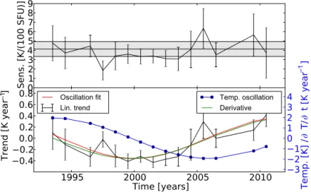
for the sensitivity derived in Sect. 4.3 for the fit using the solar cycle and an oscillation ((4.1±0.8) K(100 SFU)−1). The sensitivities derived for the 11-year time intervals show some variations but considering the uncertainties no signifi-cant changes can be observed. The mean of the derived sensi-tivities is (3.9±0.3) K(100 SFU)−1, which agrees very well with the value derived before.

The lower panel of Fig. 14 shows the derived linear trends in black. We fit a sinusoid to these trend values (red line in figure) that results in the values A=(0.36±0.06) K for the amplitude andP=(23.2±2.5) years for the period. This oscillation found in the trend values should be equal to the

derivative of the 25-year oscillation derived in Sect. 4.3 with a reduced amplitude, since 11-year time intervals are used, so no local derivative is obtained. This agreement is indeed the case. The observed period of the trend oscillation agrees within the uncertainties with the 25-year oscillation derived in the former section and the phase is also correct. The 25-year oscillation of the temperature is shown in the lower panel of Fig. 14 in blue and the corresponding derivative in green (with a second axis to the right). It appears that the green and red curve are nearly identical. In total the analysis method using 11-year time intervals leads to the same results as the fit including the sensitivity to the solar cycle and an oscillation to the whole data series. So this analysis confirms the results obtained in Sect. 4.3.

5 Discussion

5.1 11-year solar cycle

194

196

198

200

202

204

206

208

T

[K

]

1990

1995

_{Time [years]}

2000

2005

2010

2015

4

2

0

2

4

T

[K

]

Figure 12.The upper panel of the figure shows the time series of annual average OH∗temperatures in black and the fit corresponding to

Eq. (10) with the coefficientsCsolar=(4.1±0.8) K(100 SFU)−1,Csin=(1.95±0.44) K, andP=(24.8±2.1) years in red. In the lower

panel the residualTresof the two is shown. For description of displayed uncertainties see Fig. 6

0 5 10 15 20 25 30 35

Period [years] 0

1 2 3 4 5 6 7 8

Norm. power

Figure 13.The Lomb–Scargle periodogram for the time series of

annual OH∗temperatures (see Fig. 1 lower panel) is shown in black

and the LPS for the residual after subtracting the fit according to Eq. (10) (see Fig. 12 lower panel) is shown in red. For details see description of Fig. 7.

method the results differ slightly from each other, but they nearly all agree within the uncertainties (only the value de-rived by using the Hale cycle seems to be a little too large). Since the parameters for the fits (solar radio flux, solar po-lar magnetic field, oscillation, and time) are not completely independent of each other, the derived coefficients are only approximations of the true values. A much longer time se-ries, including more solar maxima, would be necessary to finally derive the true coefficients. Thus, small differences in the derived values are expected, especially in the case of the multiple linear regression including the solar radio flux and the linear trend, since this regression leads to a result

that cannot completely explain all long-term trends and os-cillations in the time series. Nearly all derived values for the sensitivity of the OH∗temperatures to the 11-year solar cycle are slightly larger than the one derived in the former analy-sis of the GRIPS measurements at Wuppertal. However, the time intervals are different for the analyses, which can lead to different results for the derived sensitivities. This aspect was already discussed by Offermann et al. (2010).

Besides the fact that the derived values are in the expected range for the northern middle to high latitudes, one new as-pect with resas-pect to the correlation between 11-year solar cy-cle and mesopause temperatures has become apparent. In the present study the correlation was determined for three so-lar maxima including the comparably weak latest soso-lar cycle 24. Our study shows that the significant correlation between OH∗_{temperatures and the 11-year solar cycle is still evident}

in this case.

5.2 Linear trend and trend break

Temperature trends in the mesopause region are reported in a number of papers, and a review about numerous results is given by Beig (2011b, see Fig. 2 and corresponding sec-tion). The temperature trends reported there range between no trend up to a cooling of about 3 K decade−1. Recent stud-ies by different authors lead to the following results. Com-bined Na lidar observations at Fort Collins (41◦_{N, 105}◦_W)

1995

2000

_{time [years]}

2005

2010

01

23

45

67

89

Sens. [K/(100 SFU)]

1995

2000

_{Time [years]}

2005

2010

0.4

0.2

0.0

0.2

0.4

0.6

0.8

Trend [K year ]

Oscillation fit Lin. trend

3

2

1

0

1

2

3

4

Te

mp

. [K

] /

T/

t [

Ky

ea

r ]

Temp. oscillation Derivative

–1

–1

Figure 14.The upper panel shows the sensitivity to the solar activity derived for different 11-year time intervals. All values are displayed

at the middle of the corresponding time interval. The error bars show the 1σ uncertainties. The grey shaded area marks the range of the

sensitivity derived in Sect. 4.3 for the fit using the solar cycle and one oscillation (Csolar=(4.1±0.8) K(100 SFU)−1). The lower panel of

the figure shows the corresponding linear trends for each time interval in black. A sinusoid fitted to these values is shown in red. The result for the 25-year temperature oscillation (see Sect. 4.3) is shown as a blue curve and the corresponding derivative of the oscillation is shown as a green curve with a second axis to the right.

for the time interval 2000–2012. Hall et al. (2012) derived a trend of (−4±2) K decade−1 from meteor radar obser-vations over Svalbard (78◦N, 16◦E) at 90 km for the time interval 2001–2012. In a former study of the Wuppertal OH∗ _{temperature series (1988–2008) a negative trend of}

(−2.3±0.6) K decade−1was found (Offermann et al., 2010). The multiple linear regression using the solar radio flux and time as parameters in this paper results in a cooling trend of (−0.89±0.55) K decade−1for the Wuppertal OH∗ temper-atures from 1988 to 2015 (see Sect. 4.1), which is in good agreement with the observations by She et al. (2015). The value is smaller than the trend derived in the former study of the Wuppertal data. Since there has been an increase in temperature from about 2006, and the former study by Offer-mann et al. (2010) ended in 2008, this temperature increase leads to a smaller negative trend in our study. However, as shown above, one linear trend is not sufficient to account for all long-term variation in the time series. Due to this we introduced a trend break and found a negative trend be-fore 2008 and a positive trend afterwards. The obtained val-ues are (−2.4±0.7) K decade−1and (6.4±3.3) K decade−1 (see Sect. 4.2). The time interval used in the former study of the Wuppertal OH∗ _{temperature series by Offermann et al.}

(2010) is nearly identical to the time interval of the first phase, showing the negative temperature trend. The linear temperature trends derived by Offermann et al. (2010) and in this study perfectly agree for this time interval. Due to the ad-ditional 7 years of observations this study now clearly shows that the former negative linear trend turned into a positive trend in the last years. This finding is contrary to the other recent studies (She et al., 2015; Perminov et al., 2014; Hall

et al., 2012; Mokhov and Semenov, 2014), where no trend break in the mid-2000s is reported.

5.3 Long-term oscillation

The observed trend break can also be described using a long periodic oscillation. In Sect. 4.3 we show two different pos-sibilities for such a long periodic oscillation.

Firstly, the solar polar magnetic field (Hale cycle) is used as one parameter in a multiple linear regression with the second parameter being the solar radio flux. The correla-tion coefficients areCsolar=(5.0±0.7) K(100 SFU)−1 and Chale=(1.8±0.5) K(100 µT)−1 (r2=0.71). Especially at the beginning and the end of the time series the fit curve does not perfectly match the observations (see Fig. 10). Addition-ally, the LSP for the temperature residual after subtracting this fit curve still shows a peak in the long periodic range (red curve in Fig. 11), although this is not significant. Thus, the Hale cycle together with the 11-year solar cycle might not explain all observed long-term dynamics. Because of these facts, we believe that the solar polar magnetic field acting as an input parameter is not very suitable.

Secondly, an independent oscillation is used to de-scribe the OH∗ _{temperature time series. A least-square}

phase-1975 1980 1985 1990 1995 2000 2005 2010 2015 Time [years]

2 1 0 1 2 3

Temperature [K]

1988–2015

1988–2008 (Offermann et al. (2010)) 1975–2015

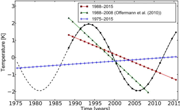
Figure 15. 25-year oscillation of OH∗ temperatures resulting from the least-square fit using Eq. (10). The coefficients are

Csin=(1.95±0.44) K, andP=(24.8±2.1) years. The solid black

line with full circles shows the oscillation for the analysed time in-terval 1988–2015 and the dashed black line shows the continuation of this oscillation back to 1975. The red line with squares displays a linear fit to the oscillation for the time interval 1988–2015, the green line with triangles the fit for the interval 1988–2008, and the blue line with plus signs a fit to the interval 1975–2015.

shifted compared to the Hale cycle and the extrema occur slightly before the extrema of the solar polar magnetic field (compare green curve in Fig. 8 and black curve in Fig. 15, e.g. maximum at about 1993 compared to 1994/1995). This time shift supports the opinion that the Hale cycle is not very likely as an acting input parameter. The nature of the 25-year oscillation is not clear yet, but a self-sustained oscillation in the atmosphere would be a real possibility. Such oscillations were recently discovered by Offermann et al. (2015). An oscillation with a period of about 20 to 25 years is found in various atmospheric parameters such as temperature (Qu et al., 2012; Wei et al., 2015), geopotential height (Coughlin and Tung, 2004a, b), and planetary wave activity (Jarvis, 2006; Höppner and Bittner, 2007). It is also seen in two atmospheric models (HAMMONIA, WACCM). A detailed discussion is, however, beyond the scope of this paper.

The most important point here is that no additional lin-ear trend can be maintained. All long-term dynamics of the Wuppertal OH∗temperature time series can be described as a combination of the 11-year solar cycle and a 25-year os-cillation. With the knowledge of this 25-year oscillation the linear trends derived in this study (see Sect. 4.1) and a former study of the Wuppertal OH∗_{temperature time series can be}

reproduced. Figure 15 demonstrates that very different trends can be obtained if specific time intervals of the (sinusoidal) data are used. By fitting a line to the corresponding part (time interval) of the data we obtain the linear trend. The linear trend for the time interval analysed in this study (1988–2015) is (−0.097±0.032) K year−1, which is the same as the lin-ear trendCtrend=(−0.089±0.055) K year−1derived by us-ing a multiple linear regression with time and solar radio flux

as parameters (see Sect. 4.1). This linear trend is shown in Fig. 15 as a red line with squares. Offermann et al. (2010) derived a linear trend for the time interval 1988–2008 of (−0.23±0.06) K year−1. A linear fit to the data for this time interval leads to a slope of (−0.22±0.03) K year−1 (green line with triangles in Fig. 15). Thus, the 25-year oscillation “explains” the derived linear trends of this and the former study as well as the obvious trend break observed in the data series. This means that all different kinds of linear trends are possible depending on the time interval which is analysed. If we continue the oscillation back to 1975 (black dashed line in Fig. 15) and fit a line to these data for the whole time interval (1975–2015; blue line with plus signs) in Fig. 15, this leads to a slope of (0.017±0.018) K year−1. This continuation is certainly an assumption and cannot be verified by the obser-vations, but it is likely and clearly shows the possible effects. The presence of such a long periodic oscillation that, in com-bination with the 11-year solar cycle, explains all long-term dynamics without an additional linear trend is very impor-tant with respect to any kind of comparison between differ-ent observations or model simulations. Each comparison of linear trends is only valid if the same time interval is anal-ysed. Furthermore, the current study suggests that there is no universal linear trend which is valid for all time intervals at this altitude.

5.4 Stability of solar sensitivity

The analysis by using different 11-year time intervals leads to two main results. Firstly, the sensitivity to the solar activ-ity is fairly stable throughout the whole time period 1988– 2015. There are some variations in sensitivity but consider-ing the uncertainties there are no significant changes. The mean of the derived values is (3.9±0.3) K(100 SFU)−1. This value is in nearly perfect agreement with the result of (4.1±0.8) K(100 SFU)−1 for the fit including the 11-year solar cycle and one oscillation using the whole data series at once. So the assumption that the sensitivity to the solar activ-ity is constant during the whole time period is valid for the Wuppertal OH∗observations.

Secondly, the derived partial trend values show the same oscillation as the derivative of the 25-year temperature os-cillation. Thus, the analysis using the 11-year time intervals confirms the result that, besides the 11-year solar cycle, an oscillation of about 25 years is the second important compo-nent of the OH∗_{temperatures observed at Wuppertal.}

6 Summary and conclusions

1. The OH∗ _{temperatures show a significant correlation}

with the solar radio flux. We find a sensitivity to the 11-year solar cycle of 3–5 K(100 SFU)−1_.

2. One linear trend during the whole time interval (to-gether with the sensitivity to the 11-year solar cy-cle) cannot sufficiently explain all long-term dynam-ics found in the OH∗ temperatures. We introduce a trend break to better account for these long-term dynamics. The best representation of the tempera-ture series is found if the trend break occurs in mid-2008 (BP=(2008.8±1.7) years). Before the break point the linear trend is negative and after the break point the trend turns positive with the slopes of (−0.24±0.07) K year−1_{and (0.64±0.33) K year}−1_. 3. The reversal of the temperature trend can also be

described by a long periodic oscillation. We present two possibilities for this oscillation. Firstly, the solar polar magnetic field of the sun (Hale cycle) is used in a multiple linear regression together with the solar radio flux as second parameter. The derived regression coefficients are Csolar=(5.0±0.7) K(100 SFU)−1 and Chale=(1.8±0.5) K(100 µT)−1 (r2=0.71). Secondly, an independent oscillation is used instead of the Hale cycle. A least-square fit leads to the coefficients Csolar=(4.1±0.8) K(100 SFU)−1, Csin=(1.95±0.44) K for the amplitude, and P =(24.8±3.3) years for the period. The most important point here is that no additional linear trend is needed.

4. Caution has to be applied when estimating linear trends from data sets containing long-term variations. Trend results are quite sensitive to the length of the data in-terval used. In such a case a piecewise linear trend ap-proach has to be used or the long-term variation has to be described in another appropriate way, e.g. by using an oscillation.

7 Data availability

The GRIPS data used in this study can be obtained by request to the corresponding author or to P. Knieling (knieling@uni-wuppertal.de). The monthly average values of the solar radio flux F10.7 cm were provided by Natural Resources Canada (Space Weather Canada) and were obtained from http: //www.spaceweather.gc.ca/solarflux/sx-5-mavg-en.php. The solar polar field strength data were provided by the Wilcox Solar Observatory and were obtained from http://wso. stanford.edu/Polar.html.

Acknowledgements. This work was funded by the German

Fed-eral Ministry of Education and Research (BMBF) within the ROMIC (Role Of the Middle atmosphere In Climate) project MALODY (Middle Atmosphere LOng period DYnamics) under Grant no. 01LG1207A. Wilcox Solar Observatory data used in this study was obtained via the web site http://wso.stanford.edu at 2016:04:11_08:31:21 PDT courtesy of J. T. Hoeksema. The Wilcox Solar Observatory is currently supported by NASA. The solar radio flux 10.7 cm data was obtained from the Natural Resources Canada, Space Weather Canada website: http://www.spaceweather.gc.ca/.

Edited by: F.-J. Lübken

Reviewed by: J. Laštovicka and one anonymous referee

References

Baker, D. J., and Stair Jr., A. T.: Rocket measurements of the al-titude distributions of the hydroxyl airglow, Phys. Scr., 37, 611, doi:10.1088/0031-8949/37/4/021, 1998.

Beig, G.: Long term trends in the temperature of the meso-sphere/lower thermosphere region: 2. Solar response, J. Geo-phys. Res., 116, A00H12, doi:10.1029/2011JA016766, 2011a. Beig, G.: Long term trends in the temperature of the

meso-sphere/lower thermosphere region: 1. Anthropogenic influences, J. Geophys. Res., 116, A00H11, doi:10.1029/2011JA016646, 2011b.

Bittner, M., Offermann, D., and Graef, H. H.: Mesopause tempera-ture variability above a midlatitude station in Europe, J. Geophys. Res., 105, 2045–2058, doi:10.1029/1999JD900307, 2000. Bittner, M., Offermann, D., Graef, H. H., Donner, M., and

Hamil-ton, K.: An 18-year time series of OH∗ rotational

tempera-tures and middle atmosphere decadal variations, J. Atmos. Sol. Terr. Phy., 64, 1147–1166, doi:10.1016/S1364-6826(02)00065-2, 2002.

Coughlin, K. and Tung, K. K.: Eleven-year solar cycle sig-nal throughout the lower atmosphere, J. Geophys. Res., 109, D21105, doi:10.1029/2004JD004873, 2004a.

Coughlin, K. T. and Tung, K. K.: 11-Year solar cycle in the strato-sphere extracted by the empirical mode decomposition method, Adv. Space Res., 34, 323–329, doi:10.1016/j.asr.2003.02.045, 2004b.

Cumming, A., Marcy, G. W., and Butler, R. P.: The lick planet search: detectability and mass thresholds, Astrophys. J., 526, 890–915, doi:10.1086/308020, 1999.

Hall, C. M., Dyrland, M. E., Tsutsumi, M., and Mulligan, F. J.:

Tem-perature trends at 90 km over Svalbard, Norway (78◦N 16◦E),

seen in one dacade of meteor radar observations, J. Geophys. Res., 117, D08104, doi:10.1029/2011JD017028, 2012.

Horne, J. H. and Baliunas, S. L.: A prescription for period analysis of unevenly sampled time series, Astrophys. J., 302, 757–763, 1986.

Höppner, K. and Bittner, M.: Evidence for solar signals in the mesopause temperature variability?, J. Atmos. Sol.-Terr. Phy., 69, 431–448, doi:10.1016/j.jastp.2006.10.007, 2007.

King, J. W.: Sun-weather relationships, Aeronautics and Astronau-tics, 13, 10–19, 1975.

King, J. W., Hurst, E., Slater, A. J., Smith, P. A., and Tamkin, B.: Agriculture and sunspots, Nature, 252, 2–3, 1974.

Lastovicka, J., Solomon, S. C., and Qian, L.: Trends in the Neutral and Ionized Upper Atmosphere, Space Sci. Rev., 168, 113–145, doi:10.1007/s11214-011-9799-3, 2012.

Lomb, N. R.: Least-squares frequency analysis of unequally spaced data, Astrophys. Space Sci., 39, 447–462, 1976.

Miyahara, H., Yokoyama, Y., and Masuda, K.: Possible link be-tween multi-decadal climate cycles and periodic reversals of solar magnetic field, Earth Planet. Sc. Lett., 272, 290–295, doi:10.1016/j.epsl.2008.04.050, 2008.

Mokhov, I. I. and Semenov, A. I.: Nonlinear temperature changes in the atmospheric mesopause region of the atmosphere against the background of global climate changes, 1960–2012, Dokl. Earth Sc., 456, 741–744, doi:10.1134/S1028334X14060270, 2014. Mursula, K. and Zieger, B.: Long term north-south asymmetry in

solar wind speed inferred from geomagnetic activity: A new type of century-scale solar oscillation, Geophys. Res. Lett., 28, 95–98, doi:10.1029/2000GL011880, 2001.

Oberheide, J., Offermann, D., Russell III, J. M., and Mlynczak, M.

G.: Intercomparison of kinetic temperature from 15 µm CO2limb

emissions and OH∗(3,1) rotational temperature in nearly

coin-cident air masses: SABER, GRIPS, Geophys. Res. Lett., 33, L14811, doi:10.1029/2006GL026439, 2006.

Offermann, D., Donner, M., Knieling, P., and Naujokat, B.:

Middle atmosphere temperature changes and the

dura-tion of summer, J. Atmos. Sol.-Terr. Phy., 66, 437–450, doi:10.1016/j.jastp.2004.01.028, 2004.

Offermann, D., Jarisch, M., Donner, M., Steinbrecht, W., and Semenov, A. I.: OH temperature re-analysis forced by recent variance increases, J. Atmos. Sol.-Terr. Phy., 68, 1924–1933, doi:10.1016/j.jastp.2006.03.007, 2006.

Offermann, D., Gusev, O., Donner, M., Forbes, J. M., Ha-gan, M., Mlynczak, M. G., Oberheide, J., Preusse, P., Schmidt, H., and Russel III, J. M.: Relative intensities of middle atmosphere waves, J. Geophys. Res., 114, D06110, doi:10.1029/2008JD010662, 2009.

Offermann, D., Hoffmann, P., Knieling, P., Koppmann, R., Ober-heide, J., and Steinbrecht, W.: Long-term trend and solar cycle variations of mesospheric temperature and dynamics, J. Geo-phys. Res., 115, D18127, doi:10.1029/2009JD013363, 2010. Offermann, D., Wintel, J., Kalicinsky, C., Knieling, P.,

Kopp-mann, R., and Steinbrecht, W.: Long-term development of short-period gravity waves in middle Europe, J. Geophys. Res., 116, D00P07, doi:10.1029/2010JD015544, 2011.

Offermann, D., Goussev, O., Kalicinsky, C., Koppmann, R., Matthes, K., Schmidt, H., Steinbrecht, W., and Wintel, J.: A case study of multi-annual temperature oscillations in the at-mosphere: Middle Europe, J. Atmos. Sol.-Terr. Phy., 135, 1–11, doi:10.1016/j.jastp.2015.10.003, 2015.

Perminov, V. I., Semenov, A. I., Medvedeva, I. V., and Zheleznov, Yu. A.: Variability of mesopause temperature from hydroxyl airglow observations over mid-latitudinal sites, Zvenig-orod and Tory, Russia, Adv. Space Res., 54, 2511–2517, doi:10.1016/j.asr.2014.01.027, 2014.

Qu, W., Zhao, J., Huang, F., and Deng, S.: Correlation between the 22-year solar magnetic cycle and the 22-year

quasicy-cle in the Earth’s atmospheric temperature, Astron. J., 144, 6, doi:10.1088/0004-6256/144/1/6, 2012.

Ryan, S. E. and Porth, L. S.: A tutorial on the piecewise regres-sion approach applied to bedload transport data, Gen. Tech. Rep., RMRS-GTR-189, Fort Collins, CO: U.S. Department of Agricul-ture, Forest Service, Rocky Mountain Research Station, 2007. Scafetta, N. and West, B. J.: Estimated solar contribution

to the global surface warming using the ACRIM TSI

satellite composite, Geophys. Res. Lett., 32, L18713,

doi:10.1029/2005GL023849, 2005.

Scargle, J. D.: Studies in astronomical time series analysis. II. Sta-tistical aspects of spectral analysis of unevenly spaced data, As-trophys. J., 263, 835–853, 1982.

Scherrer, P. H., Wilcox, J. M., Svalgaard, L., Duvall Jr., T. L., Dittmeier, P. H., and Gustafson, E. K.: The mean magnetic field of the sun – Observations at Stanford, Sol. Phys., 54, 353–361, 1977.

Schmidt, C., Höppner, K., and Bittner, M.: A ground-based spectrometer equipped with an InGaAs array for rou-tine observations of OH(3-1) rotational temperatures in the mesopause region, J. Atmos. Sol.-Terr. Phy., 102, 125–139, doi:10.1016/j.jastp.2013.05.001, 2013.

Schwarzenberg-Czerny, A.: The distribution of empirical

periodograms: Lomb-Scargle and PDM spectra, Mon.

Not. R. Astron. Soc., 301, 831–840, doi:10.1111/j.1365-8711.1998.02086.x, 1998.

She, C.-Y., Krueger, D. A., and Yuan, T.: Long-term midlatitude mesopause region temperature trend deduced from quarter cen-tury (1990–2014) Na lidar observations, Ann. Geophys., 33, 363–369, doi:10.5194/angeo-33-363-2015, 2015.

Svalgaard, L., Cliver, E. W., and Kamide, Y.: Sunspot cycle 24: Smallest cycle in 100 years?, Geophys. Res. Lett., 32, L01104, doi:10.1029/2004GL021664, 2005.

Thomas, S. R., Owens, M. J., and Lockwood, M.: The 22-year Hale cycle in cosmic ray flux – Evidence for direct heliospheric mod-ulation, Solar Phys., doi:10.1007/s11207-013-0341-5, 2013. Townsend, R. H. D.: Fast calculation of the Lomb-Scargle

peri-odogram using graphics processing units, Astrophys. J. Suppl. S., 191, 247–253, doi:10.1088/0067-0049/191/2/247, 2010. Wei, M., Qiao, F., and Deng, J.: A Quantitative Definition of Global

Warming Hiatus and 50-Year Prediction of Global-Mean Surface Temperature, J. Atmos. Sci., 72, 3281–3289, doi:10.1175/JAS-D-14-0296.1, 2015.

White, W. B., Lean, J., Cayan, D. R., and Dettinger, M. D.: Response of global upper ocean temperature to chang-ing solar irradiance, J. Geophys. Res., 102, 3255–3266, doi:10.1029/96JC03549, 1997.

Willet, H. C.: Recent statistical evidence in support of predictive significance of solar-climatic cycles, Mon. Weather Rev., 102, 679–686, 1974.

Zechmeister, M. and Kürster, M.: The generalised Lomb-Scargle periodogram – A new formalism for the floating-mean and Keplerian periodograms, Astron. Astrophys., 496, 577–584, doi:10.1051/0004-6361:200811296, 2009.