www.earth-syst-dynam.net/6/311/2015/ doi:10.5194/esd-6-311-2015
© Author(s) 2015. CC Attribution 3.0 License.
Exploring objective climate classification for the
Himalayan arc and adjacent regions using gridded data
sources
N. Forsythe, S. Blenkinsop, and H. J . Fowler
Centre for Earth Systems Engineering Research (CESER), School of Civil Engineering and Geosciences, Newcastle University, Newcastle, UK
Correspondence to:N. Forsythe ([email protected])
Received: 9 September 2014 – Published in Earth Syst. Dynam. Discuss.: 29 September 2014 Revised: 10 March 2015 – Accepted: 9 April 2015 – Published: 28 May 2015
Abstract. A three-step climate classification was applied to a spatial domain covering the Himalayan arc and adjacent plains regions using input data from four global meteorological reanalyses. Input variables were selected based on an understanding of the climatic drivers of regional water resource variability and crop yields. Principal component analysis (PCA) of those variables andk-means clustering on the PCA outputs revealed a reanalysis
ensemble consensus for eight macro-climate zones. Spatial statistics of input variables for each zone revealed consistent, distinct climatologies. This climate classification approach has potential for enhancing assessment of climatic influences on water resources and food security as well as for characterising the skill and bias of gridded data sets, both meteorological reanalyses and climate models, for reproducing subregional climatologies. Through their spatial descriptors (area, geographic centroid, elevation mean range), climate classifications also provide metrics, beyond simple changes in individual variables, with which to assess the magnitude of projected climate change. Such sophisticated metrics are of particular interest for regions, including mountainous areas, where natural and anthropogenic systems are expected to be sensitive to incremental climate shifts.
1 Introduction
The first objective, quantitative systems for global climate classification were developed in the early 20th century by integrating climate data to delineate zones of coherent veg-etation type or ecoregion (Belda et al., 2014). By distill-ing information from multiple climate variables which af-fect vegetation typology, climatic classifications can provide a framework for understanding natural resource systems (El-guindi et al., 2014). By focusing specifically on climate vari-ables which govern river flows and crop growth, derived cli-mate classifications can also yield insight into the depen-dency of agricultural production on water resources. How-ever, the bulk of recent literature (e.g. Chen and Chen, 2013; Mahlstein et al., 2013; Zhang and Yan, 2014) is global in scope. In this study we focus for the first time on a specific classification for the Himalayan arc and adjacent regions,
concentrating on climate types relevant to the spatial domain and time period of interest.
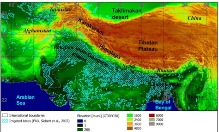
Figure 1. Geographic context of the study area (Himalayan arc and adjacent plains) including elevation and areas with > 33 % un-der irrigation (hatched). Data sources include the United Nations Food and Agriculture Organization (FAO) and the United States Geological Survey Global 30 Arc-Second Digital Elevation Model (GTOPO30).
al. (2010) point out that the semi-arid plains of the Lower In-dus had only marginal (rainfed) agricultural viability until the development of irrigation infrastructure. Irrigation demand in the Lower Indus is supplied by run-off from the Hindu Kush, Karakoram and western Himalaya. Thus holistic understand-ing of regional food security depends upon characterisation of the spatial as well as climatological differences of these hydrologically connected subregions. Furthermore, it is pos-sible that these subregions will experience distinct trajecto-ries of change in the coming decades. Differential rates, or even signs, of change could substantially alter the regional balance of irrigation water supply and demand. The climate classification approach offers a framework within which to evaluate such water balance scenarios.
Global meteorological reanalyses provide coherent syn-theses of atmospheric states including radiative and mass flux exchanges with the sea or land surface. In this paper we compare the climatologies described for the study area from four reanalyses – JRA-55 (Ebita et al., 2011), ERA-Interim (Dee et al., 2011), NASA MERRA (Rienecker et al., 2011) and NCEP CFSR (Saha et al., 2011) – which encom-pass the recent decades rich in data from both ground-based and satellite-borne instruments. In assessing climate classi-fications derived from each reanalysis we are not only in-terested in how the climatically defined zones relate to water resource supply (mountainous headwaters) and demand (irri-gated plains) areas but also in how the classifications derived from individual reanalyses relate to each other. These inter-comparisons establish a methodology for evaluating gridded data sets, including global and regional climate simulations (Elguindi et al., 2014) as well as reanalyses. Comparisons can be made not only between different models but also be-tween different time periods (“time slices”), for either his-torical data sets (Belda et al., 2014; Chen and Chen, 2013)
or simulations by climate models (Mahlstein et al., 2013). Temporal changes in derived climate zones can be assessed in terms of both projected spatial changes (areal extent, ele-vation range, etc.) and of projected climatic changes (mean, annual range, etc.) in the individual climate variables used to create the classification.
2 Data and methods
2.1 Reanalysis data sets
Reanalyses are generally conducted by institutions respon-sible for meteorological forecasting and are undertaken in part to assess the performance forecasting models and the data assimilation systems which support them (Uppala et al., 2005). The resulting coherent multi-decadal syntheses of cli-mate conditions, however, are of substantial utility to a much broader spectrum of natural scientists. In this study we draw upon data from four reanalyses produced by agencies from diverse geographic regions. Characteristics of the reanaly-ses used in this study are provided in Table 1 and differ in both spatial and temporal resolutions. Given the forecast-driven nature of reanalyses, it is common for time steps to be organised in 6 h synoptic forecasting time windows. The NASA MERRA data set is distinct in that the default time step is hourly. In all cases daily means were calculated as the mean of the available sub-daily time steps. Daily max-imum and minmax-imum were taken as the highest and lowest values respectively amongst the sub-daily time steps unless reported specifically, as was the case for NCEP CFSR. Di-urnal range was calculated as maximum minus minimum. In order to make extracted climatic values as comparable as possible, a common reference period, 1980 to 2009, avail-able from each of the reanalyses, was selected for this study. However, comparability of the results was still limited by dif-fering spatial resolutions of the reanalyses as both tempera-ture and precipitation are greatly influenced by topography in mountainous regions (Immerzeel et al., 2012). The fidelity with which each reanalysis reproduces the topography of the study area is limited by its spatial resolution. For this reason, the JRA-55 (1.25×1.25◦resolution) data set is expected to be handicapped compared to the NCEP CFSR (0.50×0.50 decimal degree resolution) data set. Nevertheless, other el-ements, including efficacy of data assimilation and realism of land-surface process algorithms, are also expected to play substantial roles in determining reanalysis skill.
2.2 Selection of climate variables governing water resources and food security
Table 1.Reanalysis data sets utilised for comparative climate classification.
Reanalysis Producer Time period covered Spatial resolution (◦) Diurnal discretisation
JRA-55 JRA 1958 to (near) present 1.25×1.25 6 h synoptic forecast/analysis periods
ERA-Interim ECMWF 1979 to (near) present 0.75×0.75 6 h synoptic forecast/analysis periods CFSR NCEP 1979 to 2009 (later extended) 0.50×0.50 6 h synoptic forecast/analysis periods
MERRA NASA 1979 to (near) present 0.67×0.50 hourly
the key climatic factors involved (e.g. Nolan et al., 2008). In this paper the processes of interest are river flows from mountainous headwaters and agricultural production, both of which depend upon inputs of mass (precipitation) and energy (ambient temperature and incoming radiation). From a sim-ulation standpoint, common approaches for modelling both meltwater generation from seasonal snowpack and glaciers (Ragettli et al., 2013) and crop yields (Baigorria et al., 2007; Kar et al., 2014) require both air temperature and incom-ing radiation in addition to precipitation as input data. Fur-thermore, moisture exchanges from the land surface and at-mosphere depend upon the latter’s vapour pressure deficit, which is commonly expressed as relative humidity. Whilst these parameters can be observed directly, the diurnal tem-perature range (DTR) also acts as an effective proxy for am-bient moisture conditions (Easterling et al., 1997).
In establishing the methodology used here, we favoured reanalysis variables with the simplest relationship to com-monly observed parameters at ground-based stations. Hence,
Tavg(mean temperature) and DTR – which together describe
the diurnal temperature cycle and can be calculated at sta-tions recording solelyTmax(maximum temperature) andTmin
(minimum temperature) – along with precipitation were se-lected as governing variables. An exception to this princi-ple was made in selecting net incoming shortwave radiation (SWnet) at the ground surface as a governing variable due to the importance of seasonal snow cover in the hydrologi-cal regimes of major Himalayan and Tibetan river systems. SWnet can be observed at standard manned meteorological stations and automatic weather station (AWS) units if they are equipped with radiometers, but is also indirectly available from remote sensing via albedo and cloud climatology. It was largely for the linkage between SWnet and snow cover via albedo that the former was selected as a key variable. Specif-ically, land surfaces with full snow cover have a much higher albedo than “bare ground” and albedo evolves during snow-pack accumulation and ablation when snow cover is partial. Albedo in turn modulates net shortwave absorption from in-coming solar radiation at the surface. Thus net shortwave ra-diation can serve as a proxy for snow cover. The linkage be-tween SWnetand cloud cover is also useful, as the latter is an indicator of large-scale weather system – mid-latitude west-erly or tropical monsoon – influence. Cloud cover influences SWnetby modulating the amount of incoming shortwave ra-diation reaching the surface. In the absence of snow cover,
suppression of SWnetin summer months over South Asia is likely due to monsoonal activity, while suppression in other months suggests mid-latitude westerly disturbances. Table 2 lists the governing variables selected for this study, includ-ing the seasonal aggregates of interest, and summarises their physical significance.
Prior to derivation of climate classifications, a comparison of the climatologies from the individual reanalyses provides a context within which differences can be interpreted. To es-tablish a common framework, the “native” resolution data from each reanalysis was regridded (subdivided) to a com-mon 0.25×0.25◦ spatial resolution. Ensemble means were calculated, by grid cell, from the simple averages of the four reanalyses. There was no weighting applied from any met-ric of skill or confidence, nor were any corrections made to account for differences between “native” orography and esti-mated surface elevation of the target common grid cell. This approach was taken in the absence of detailed information on likely biases by the reanalyses in the variables of interest. Once the ensemble mean had been calculated, normalised differences, i.e. individual reanalysis value minus ensemble mean, were calculated to facilitate comparisons of individual climatologies.
Table 2.Variables used for Himalayan region climate classification.
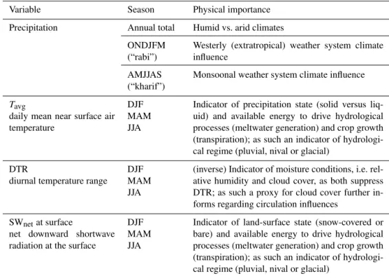
Variable Season Physical importance
Precipitation Annual total Humid vs. arid climates
ONDJFM (“rabi”)
Westerly (extratropical) weather system climate influence
AMJJAS (“kharif”)
Monsoonal weather system climate influence
Tavg
daily mean near surface air temperature
DJF MAM JJA
Indicator of precipitation state (solid versus liq-uid) and available energy to drive hydrological processes (meltwater generation) and crop growth (transpiration); as such an indicator of hydrologi-cal regime (pluvial, nival or glacial)
DTR
diurnal temperature range
DJF MAM JJA
(inverse) Indicator of moisture conditions, i.e. rel-ative humidity and cloud cover, as both suppress DTR; as such a proxy for cloud cover further in-forms regarding circulation influences
SWnetat surface
net downward shortwave radiation at the surface
DJF MAM JJA
Indicator of land-surface state (snow-covered or bare) and available energy to drive hydrological processes (meltwater generation) and crop growth (transpiration); as such an indicator of hydrologi-cal regime (pluvial, nival or glacial)
and NASA MERRA show the opposite pattern, with ERA-Interim being much wetter over the Nepal–Bhutan–China border region and NASA MERRA being much drier over the Terai, Assam and Ganges–Brahmaputra Delta.
While adequate moisture inputs from precipitation are pre-requisite for both river flows and agricultural production, the role of energy inputs in both the generation of meltwa-ter runoff, from snow and glacial ice, and driving crop de-velopment, through photosynthesis and transpiration, is also critical. Figure 3 shows the ensemble mean climatologies and individual (normalised difference) contributions for win-ter (December to February) SWnet, spring (March to May) dailyTavgand summer (June to August) DTR. These
tempo-ral aggregates (winter, spring and summer) were selected to identify hydrological regimes (pluvial, nival (snowpack) or glacial) and growing seasons dependent upon thermal condi-tions. As described in Table 2, all three seasonal values (win-ter, spring, summer) for each of these variables –Tavg, SWnet
and DTR – were used as input to the classification procedure. Figure 3 shows a single seasonal example of each variable to illustrate the information it contributes. Autumn (September to November) seasonal aggregates were not used as they are very similar to spring (mirror image) in terms of magnitude and variability and thus not expected to substantially increase information content available to the PCA.
Figure 3 shows that winter SWnetillustrates the influence of seasonal snow cover via albedo. As expected there is a generally latitudinal gradient, with decreasing SWnet mov-ing northward, although the latitudinal gradient is smaller
than reductions in net surface absorption in areas with sea-sonal snow cover. JRA-55 shows generally lower SWnet val-ues than the ensemble mean, particularly over south-western Pakistan and the Tibetan Plateau. The former difference is likely due to greater reanalysis estimates of cloud radiative effect (CRE), while over Tibet this might be due to either CRE or higher predicted albedo from greater assumed sea-sonal snow cover. In contrast JRA-55 shows higher SWnet over the Pamir and sections of the high Karakoram and Hi-malayan arc. This may be due to either assumed lesser sea-sonal snow cover (decreased albedo) or estimated clearer sky conditions (decreased CRE). Broadly speaking, ERA-Interim and NASA MERRA show the opposite contribution patterns to JRA-55, and hence detailed examination of ra-diation modulating physical mechanisms, e.g. clear versus overcast conditions and full snow cover versus bare ground, would likely reveal opposing tendencies. Between ERA-Interim and NASA MERRA, the former shows broader and more pronounced decreases in SWnetcontinuously along the Himalayan arc from Pamir through the east of Bhutan to the Sikkim. NCEP CFSR shows a mixed pattern of SWnet, agree-ing with JRA-55 north of approximately 30◦N and more closely corresponding to ERA-Interim and NASA MERRA south of this line.
The ensemble mean climatology of spring dailyTavg
dis-plays the expected influence of elevation, with sub-freezing temperatures found roughly above 3000 m a.s.l. Like SWnet,
Tavg through the freezing isotherm provides a spatial
Figure 2.Ensemble precipitation climatology and normalised com-parison of individual contributions from reanalyses used in this study. ONDJFM is the abbreviation for the period from October to March, referred to regionally as “rabi”. AMJJAS is the abbrevi-ation for the period from April to September, referred to regionally as “kharif”.
quantifies the available energy to drive melting of snow and ice as well as plant development. Although NASA MERRA is notably warmer than the other three reanalyses over the Indo-Gangetic Plain, the largest discrepancies are along Hi-malayan arc as well as at the transition from the Taklimakan Desert to the Tibetan Plateau. JRA-55 and NCEP CFSR are generally colder than the mean along the Himalayan arc but warmer along the northern Tibetan fringe. ERA-Interim is strongly warmer along the Himalayan arc but much cooler over the southern Taklimakan. NASA MERRA has more mixed contributions, with relatively limited areas showing substantial departures from the ensemble mean.
Summer DTR is not a direct indicator of energy input to the hydro-climatological system and biosphere. It does, how-ever, provide a measure of the amplitude of energy variation throughout the diurnal cycle as well as providing a proxy for relative humidity (vapour pressure deficit) and cloud cover. Examination of the ensemble mean summer DTR climatol-ogy clearly illustrates the influence of both cloud cover and humidity. Regionally summer DTR is lowest over the Ara-bian Sea and Bay of Bengal and highest over the western Central Asian deserts. Suppression of summer DTR is clearly evident by comparing the ensemble mean summer DTR in Fig. 3 to the ensemble mean monsoonal precipitation accu-mulations in Fig. 2. The influence of diurnal discretisation (sub-daily time step) on individual reanalysis DTR clima-tologies is evident in Fig. 3. NASA MERRA, with an hourly time step, has much larger DTR values over land than the
en-Figure 3.Ensemble energy input (temperature and radiation) cli-matology and normalised comparison of individual contributions from reanalyses used in this study. SWnetis net downward
short-wave radiation at the surface.Tavgis daily mean near surface air
temperature. DTR is diurnal temperature range. DJF is the (winter) period December through to February. MAM is the (spring) period March through to May. JJA is the (summer) period June through to August.
semble mean but lower DTR values than the mean over the Arabian Sea and the Bay of Bengal. MERRA’s hourly time step allows better representation of the full amplitude of the DTR, while the 6 h time steps of the other reanalyses “flat-ten” or dampen estimated diurnal variations. NCEP CFSR has the lowest DTR values, with particularly small DTR es-timates over the Central Asian deserts and Tibetan Plateau. ERA-Interim has broadly, if moderately, lower DTR values than the mean except over the Central Asian deserts as well as the Arabian Sea and Bay of Bengal. JRA-55 is similar to ERA-Interim in DTR estimates, albeit spatially more vari-able and closer to the ensemble mean.
data sets, its internal coherence, i.e. relative spatial and tem-poral variability, may still be substantial. This coherence can be tested through the climate classification process. Where good ground-based observations exist and can be translated meaningfully to the grid cell resolution in the reanalyses, bias assessment could be performed. This would provide insight into which data set more accurately represents regional con-ditions but would be very challenging and time-consuming due to data paucity and inconsistencies. This in fact high-lights one of the major benefits of the climate classifica-tion procedure: objective delineaclassifica-tion of the regional domain should enable optimisation of the use of limited ground data by defining “areas of relevance” within which the magnitude and distribution of bias can be meaningfully summarised.
2.3 Method for climate classification
The climate classification methodology used in this study directly transfers the method developed by Blenkinsop et al. (2008) for the European FOOTPRINT project, albeit with the set of variables described in Sect. 2.2 rather than those identified for FOOTPRINT (Nolan et al., 2008). Blenkinsop et al. (2008) applied a three-step approach to climate zon-ing: (i) identification of key climatic variables, (ii) principal component analysis (PCA) and (iii) k-means cluster
anal-ysis. The decision to use the PCA and k-means approach,
which classifies the spatial domain based on relative differ-ences, rather than to apply a classification based on abso-lute thresholds, e.g. Köppen–Trewartha (Belda et al., 2014), was made due to the expectation that the spatial aggregation (large grid cells) within the reanalyses would introduce in-evitable biases. These biases could be further exacerbated by the formulation of data assimilation and forecasting al-gorithms adopted by each reanalysis. Thus it seemed more reasonable to apply a relative differentiation rather than an absolute, fixed standard.
As explained by Blenkinsop et al. (2008), PCA is a nec-essary step in the climate classification process in order to reduce the dimensionality of the input variables, which are expected to be substantially correlated as a set. Prior to PCA all input variables were standardised (subtraction of spatial mean and division by spatial standard deviation). Standardis-ation was performed so that the unit-dependent absolute val-ues of the individual variables would not distort their weight-ing within the PCA process. PCA was performed usweight-ing the “mlab” module of matplotlib (Hunter, 2007) executed in a Python environment. Input and output operations of reanaly-sis data stored as GeoTiffs were handled using the RasterIO Python module (Holderness, 2011).
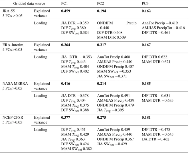
The results of the PCA for each reanalysis are summarised in Table 3. A decision was made to retain principal compo-nents (PCs) which accounted for at least 5 % of the total vari-ance in the input data set. Table 3 indicates that ERA-Interim and NCEP CFSR each had four PCs which met this criterion while JRA-55 and NASA MERRA had five PCs. Details on
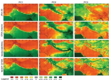
Figure 4.Comparison of the first three principal components (PCs) from each of the reanalyses used in this study. PCs are calculated from the principal component analysis (PCA) input standardised variables using the PCA output weighting factors. PCs are thus di-mensionless and values are expressed in standard deviations.
the first three PCs, which together account for between 81 and 85 % of the total variance, for each reanalysis are pro-vided in Table 3, while Fig. 4 shows these PCs graphically. The first PC for all four reanalyses was primarily composed of variables related to energy inputs (daily mean temperature, net shortwave radiation), although JRA-55, ERA-Interim and NASA MERRA all had substantial negative contributions from summer DTR. The first PC accounted for between 36 and 46 % of the total variance depending on the reanalysis chosen. As can be seen in Fig. 4, the differences between the reanalyses in spatial distribution of PC1 within the domain can be largely accounted for by the respective differences in spatial resolution. Even without allowing for the spatial reso-lution, differences in the consistency in PC1 between reanal-yses are striking.
sub-Table 3.Comparison of results of principal component analysis.
Gridded data source PC1 PC2 PC3
JRA-55 5 PCs > 0.05
Explained variance
0.459 0.194 0.162
Loading JJA DTR−0.359
DJFTavg0.380
DJF SWnet0.384
ONDJFM Precip
−0.440 DJF DTR 0.408 MAM DTR 0.509
AnnTot Precip−0.419 AMJJAS PrecipTot−0.416 DJF DTR−0.461
ERA-Interim 4 PCs > 0.05
Explained variance
0.364 0.317 0.167
Loading JJA DTR −0.353
DJFTavg0.443
MAMTavg0.404
DJF SWnet0.402
AnnTot Precip 0.460 AMJJAS Precip 0.440 ONDJFM Precip 0.407 MAM SWnet−0.353 JJA SWnet−0.371
DJF DTR 0.622 MAM DTR 0.621
NASA MERRA 5 PCs > 0.05
Explained variance
0.416 0.214 0.185
Loading JJA DTR−0.378
DJFTavg0.404
MAMTavg0.375
DJF SWnet0.388
AnnTot Precip 0.491 AMMJAS Precip 0.439 ONDJFM Precip 0.479 JJATavg−0.395
DJF DTR−0.631 MAM DTR−0.635
NCEP CFSR 5 PCs > 0.05
Explained variance
0.377 0.275 0.181
Loading DJFTavg0.451
MAMTavg0.429
JJATavg0.363
DJF SWnet0.424
MAM SWnet0.382
AnnTot Precip 0.459 AMJJAS Precip 0.440 ONDJFM Precip 0.367 JJA SWnet−0.429
DJF DTR−0.478 MAM DTR−0.645 JJA DTR−0.462
NB: rows labelled “Explained variance” indicate fraction of total input variance accounted for by the principal component (PC). Rows labelled “Loading” indicate input variables whose (coefficient) contribution to the PC is >0.35. Loading coefficients are shown with their signs to differentiate between variables with opposing contributions.
stantial differences between reanalyses in PC3. In JRA-55 the signs of Central Asian deserts and Tibetan Plateau are reversed compared to the patterns found in PC3 in the other three reanalyses. For all reanalyses, PC2 accounted for be-tween 19 and 32 % of total variance, while PC3 accounted for between 16 and 19 %. Overall the spatial patterns in Fig. 4 are physically plausible, especially PC1 (mean annual tem-perature/energy input) and PC2 (annual total precipitation) in the three similar reanalyses (excluding JRA-55). Spatial patterns in PC3 (cold season/rabi DTR) are also physically plausible, although visually they are less intuitive as diur-nal temperature cycles are substantial even in high-elevation areas (Karakoram, Himalaya, Tibetan Plateau) in these sea-sons. They are of lesser amplitude, however, than those ex-perienced currently in the Indo-Gangetic Plain and Central Asian deserts.
K-means cluster analysis was also performed using
mat-plotlib (Hunter, 2007) and RasterIO (Holderness, 2011) within a Python environment. As suggested by Blenkinsop
et al. (2008), standardised grid cell latitude and longitude were added to the retained principal components as input to the clustering process. Becausek-means cluster analysis
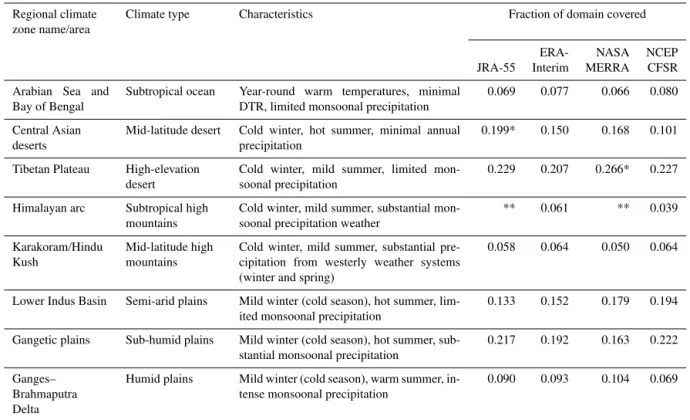
Table 4.Description of primary Himalayan region climate zones (eight clusters).
Regional climate zone name/area
Climate type Characteristics Fraction of domain covered
ERA- NASA NCEP JRA-55 Interim MERRA CFSR
Arabian Sea and Bay of Bengal
Subtropical ocean Year-round warm temperatures, minimal DTR, limited monsoonal precipitation
0.069 0.077 0.066 0.080
Central Asian deserts
Mid-latitude desert Cold winter, hot summer, minimal annual precipitation
0.199* 0.150 0.168 0.101
Tibetan Plateau High-elevation desert
Cold winter, mild summer, limited mon-soonal precipitation
0.229 0.207 0.266* 0.227
Himalayan arc Subtropical high mountains
Cold winter, mild summer, substantial mon-soonal precipitation weather
** 0.061 ** 0.039
Karakoram/Hindu Kush
Mid-latitude high mountains
Cold winter, mild summer, substantial pre-cipitation from westerly weather systems (winter and spring)
0.058 0.064 0.050 0.064
Lower Indus Basin Semi-arid plains Mild winter (cold season), hot summer, lim-ited monsoonal precipitation
0.133 0.152 0.179 0.194
Gangetic plains Sub-humid plains Mild winter (cold season), hot summer, sub-stantial monsoonal precipitation
0.217 0.192 0.163 0.222
Ganges– Brahmaputra Delta
Humid plains Mild winter (cold season), warm summer, in-tense monsoonal precipitation
0.090 0.093 0.104 0.069
*Combination of two climate zones in this reanalysis. **Not identified by this reanalysis.
3 Results
3.1 Description of emergent regional climate zones and subdivisions
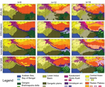
Figure 5 shows the results ofk-means clustering for each
re-analysis for 8, 12 and 16 clusters. Similar subdivisions of the eight subregional climate zones tend to emerge in all the re-analyses as cluster numbers increase, although subdivisions first emerge dependent upon spatial discretisation and clima-tological differences – illustrated in Figs. 2 and 3 – of each reanalysis.
The general characteristics of the eight emergent subre-gional climate zones are described Table 4 along with the fraction of the spatial domain each covers in each reanal-ysis (for the eight-cluster case). With the exception of the Himalayan arc zone, which was not identified by both JRA-55 and NASA-MERRA when the number of clusters was limited to eight, there is substantial agreement not only on the broad geographic locations of the eight zones but also on their spatial extent within the domain. There is arguably some blurring in the definition of the “Lower Indus Basin” (semi-arid plains), which regionally could be seen as a tran-sitional zone between the “Central Asian deserts” and the “Gangetic plains” (sub-humid plains), although the latter could itself be seen as a transitional zone between the Lower Indus and the “Ganges–Brahmaputra Delta” (humid plains).
3.2 Comparison of climatologies of emergent subregional climate zones
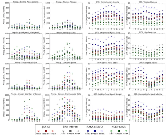
The spatial mean and ranges (minimum and maximum) have been calculated for the period monthly means of the four input variables from each reanalysis. The annual cycles of precipitation and DTR are shown in Fig. 6. The annual cy-cles of daily mean temperature and net shortwave radiation are shown in Fig. 7. Placement of subregional zones within these figures are deliberate in their relationship to geograph-ical location and large-scale circulation influences. The most northerly zones are in the upper figure panels, and the most southerly at the bottom. Zones with greater westerly weather system influence are in the left-hand column, while greater monsoonal influence zones are to the right. Results shown in both figures are referred to in the discussion throughout this section.
3.2.1 Precipitation climatologies of emergent subregional climate zones
re-Figure 5.Comparison of climate classifications resulting from the use of 8, 12 and 16 clusters (k) on principal components from the
individual reanalyses. Large units in the legend refer to zones for thek=8 case.
ceives moderate precipitation from westerly weather systems in late winter (February) and spring. The Karakoram/Hindu Kush zone is the next wettest with dominant inputs from rabi westerly weather systems and limited summer rainfall. The Tibetan Plateau has a similar seasonal distribution of pre-cipitation to the Himalayan arc but with lower monthly to-tals. The Lower Indus Basin and Central Asian deserts are the driest zones. Spread in spatial means between reanaly-ses is substantial for all climate zones and appears roughly proportional to precipitation amount, i.e. the largest spread is found in the wettest months and in the wettest zone (Ganges– Brahmaputra Delta).
3.2.2 DTR climatologies of emergent subregional climate zones
As explained in Sect. 2.2, ensemble spread in DTR cli-matologies can be substantially attributed to issues of sub-diurnal discretisation. For all climate zones except the Ara-bian Sea and Bay of Bengal, the reanalysis with an hourly time step (NASA MERRA) has the largest DTR values. Despite similar sub-diurnal discretisation, NCEP CFSR has consistently lower DTR values across all climate zones than ERA-Interim and JRA-55, which tend to agree closely with one another. Despite this considerable ensemble spread in ab-solute values, the “shape” of annual DTR cycles within cli-mate zones is consistent between reanalyses, i.e. standard-ised values are very similar. Zones with substantial mon-soonal influence – the Ganges–Brahmaputra Delta, Gangetic plains and Himalayan arc – have annual DTR minima in summer. In contrast, drier and more westerly dominated sub-regional zones – the Central Asian deserts, Tibetan Plateau,
Karakoram/Hindu Kush and Lower Indus Basin – have an-nual DTR minima in winter, although the Lower Indus has a sufficient monsoonal influence for a minor minimum (limited DTR suppression) in summer. The Arabian Sea and Bay of Bengal have the smallest DTR values both in absolute terms (annual mean) and amplitude of annual cycle.
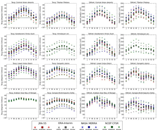
3.2.3 Daily mean temperature climatologies of emergent subregional climate zones
Based on the PCA results presented in Sect. 2.3, differ-ences in energy inputs account for the largest fraction of variance within the input data. Differences in annual cy-cles of daily Tavg provide clear differences between the
emergent subregional climate zones. The Arabian Sea and Bay of Bengal have year-round moderately warm temper-atures with minimal spread in both ensemble mean and in spatial spread within individual reanalyses. The Ganges– Brahmaputra Delta has similar monthly spatial mean values to the Arabian Sea but with incrementally larger ensemble spread and much greater spatial spread. The spatial spread is attributed to the topographic diversity within the zone, stretching from coastal areas to the front ranges of the Hi-malaya. The Lower Indus Basin and Gangetic plains have quite similar annual cycles of daily mean temperature. Both have mild cold seasons (rabi) and hot summers with large spatial spreads in all months. The ensemble spread is incre-mentally larger in all months for the Lower Indus than for the Gangetic plains. The remaining four zones – the Central Asian deserts, Tibetan Plateau, Karakoram/Hindu Kush and Himalayan arc – are alike in several months of the annual cy-cle, with mean temperatures below freezing. Ensemble and spatial spreads are greater in the Central Asian deserts and Karakoram/Hindu Kush than in the Tibetan Plateau, which is consistently the coolest zone. For the Himalayan arc, ERA-Interim and NCEP CFSR agree closely for both the spatial means and the considerable spatial spreads of this zone.
3.2.4 Net shortwave radiation climatologies of emergent subregional climate zones
Figure 6.Ensemble spatial statistics for annual cycles of precipitation (left) and DTR (right) by climate zone (eight clusters). DTR is diurnal temperature range.
by large CRE linked to monsoonal activity. This is particu-larly visible in the Ganges–Brahmaputra Delta and Gangetic plains and still noticeable in the Himalayan arc and Arabian Sea. The effect is present, though barely perceptible, in the Lower Indus Basin.
3.2.5 Commonalities and distinctions in the
climatologies of emergent subregional climate zones
The layout of Figs. 6 and 7 is intended to facilitate compari-son of adjacent climate zones. Climate zones are represented within Figs. 6 and 7 moving from north to south by moving from top to bottom panels. Given the latitudinal influence on temperature, zones with similar temperature regimes, e.g. the Lower Indus Basin and Gangetic plains, are laterally ad-jacent. In contrast, the dependence of precipitation on atmo-spheric circulation can be examined by comparing these ad-jacent panels. Thus the Lower Indus Basin, with limited mon-soonal rainfall, is found by the clustering process to be dis-tinct from the Gangetic plains. Similarly the Tibetan Plateau is distinguished from the Central Asian deserts not only by cooler temperatures but also by greater monsoonal precipi-tation. The Karakoram/Hindu Kush and Himalayan arc have similar temperature regimes, but the seasonality and magni-tude of annual precipitation, driven by the differing circula-tion influences, clearly separates them. Even without
knowl-edge of land or sea presence, the Ganges–Brahmaputra Delta zone is distinct from the Arabian Sea zone by both precipita-tion and DTR.
4 Discussion
4.1 Insights from climate classifications for water resources and food security in South Asia
The PCA andk-means clustering approach applied to climate
Figure 7.Ensemble spatial statistics for annual cycles ofTavgand SWnetby climate zone (eight clusters). SWnetis net downward shortwave
radiation at the surface.Tavgis daily mean near surface air temperature.
the Himalayan arc is upstream of the Gangetic plains and Ganges–Brahmaputra Delta. The precipitation climatologies of individual climate zones presented in Fig. 6 confirm that the Lower Indus Basin receives substantially less direct pre-cipitation than the other two plains climate zones. In a first-order analysis, irrigated areas in the Lower Indus, shown in Fig. 1, are thus much more dependent upon upstream flows than their Gangetic counterparts.
This general assessment does not, however, take into ac-count the question of intra-annual (inter-seasonal) water transfers, as the annual cycle of Ganges Basin tributary river flows will closely follow the annual precipitation cycle. Thus, in the absence of impounding reservoirs or substan-tial groundwater recharge, only limited water volumes would be available to supplement irrigation in the dry rabi season. This study also does not take into account inter-annual vari-ability, as the climate classifications here draw solely upon period means (1980 to 2009). A further limitation of this as-sessment is that at the “parcel scale” of rainfed agriculture the convective precipitation in monsoonal weather systems has very large spatial variability (Khan et al., 2014). Thus, while farmers in the irrigated Lower Indus Basin rely upon upstream flows for the bulk of crop moisture requirements, farmers in the Gangetic plains may find supplementary ir-rigation critical to compensate for spatially and temporally acute precipitation deficits and ensure crop yields.
4.2 Utility of climate classification for assessment of gridded data sets
The ensemble reanalysis input climatologies and normalised difference contributions shown in Figs. 2 and 3 illustrate the initial steps in comparative assessment of gridded data sets for bias characterisation and validation. Further logical steps would draw upon the climate zones derived through the PCA andk-means clustering approach to subdivide the spatial
do-main in order to focus and organise the use of limited in situ data (ground-based, point observations) to characterise sub-regional data set performance. The use of in situ data to pro-vide “ground truthing” and related large-scale data sets to local conditions will remain crucial for the foreseeable fu-ture because gridded data sets of a global nafu-ture – be they reanalyses, spatially interpolated from local observations, or derived from satellite imagery – will inevitably have intrin-sic biases. These biases are a function of spatial and temporal resolution of the source observations as well as the physical nature of those observations. In situ data, be they from na-tional monitoring networks or internana-tional databases such as the Global Historical Climatology Network (Lawrimore et al., 2011), could be grouped by the derived climate zones and in this way structure the analysis of statistics of “grid cell ver-sus station” biases. In this way individual gridded data sets could be assessed to determine in which subregional climate zones they perform well or poorly. This approach also per-mits comparative evaluation of different gridded data sets to determine which most accurately reproduces the climatology of a given climate zone.
This proposed methodology for bias assessment is depen-dent, however, upon the availability of station data, which are representative of climatic conditions in absolute terms at the grid-scale level. This constraint could be prohibitive for mountainous areas, such as the Karakoram/Hindu Kush, where meteorological stations are often located in valley bot-toms, substantially below the mean elevations of overlying data source grid cells. One such example is the Upper Indus Basin (Gilgit–Baltistan administrative district of Pakistan), where Archer (2003, 2004) and Archer and Fowler (2004, 2008) found climate observations at manned meteorologi-cal stations of the Pakistan Meteorologimeteorologi-cal Department lo-cated in valley settlements to correlate strongly with variabil-ity in hydrological conditions, although runoff volume fluc-tuations did not equate directly to precipitation anomalies. Thus, in mountainous or other highly spatially variable do-mains, “transfer functions” (scaling relationships) represent-ing climate parameter variation with topography may still be necessary to compare in situ point observations to grid cell spatial means in absolute terms.
These challenges for relating point-based observations to gridded data in fact point toward the utility of inter-comparison of spatial data sets. The climate classification approach provides a supplementary dimension in which to compare gridded data sets. To illustrate this, the subregional
Figure 8.Comparison of climate classifications resulting from the use of eight clusters on principal components of the control period (1970 to 1999) from the individual members of the Hadley Centre RQUMP perturbed physics ensemble downscaled over South Asia.
Table 5.Variability in primary Himalayan region climate zones (eight clusters) in the Hadley Centre downscaled perturbed physics ensemble, Regionally Quantify Uncertainty in Model Predictions (RQUMP), for South Asia.
Central Lower Karakoram/ Ganges–
Ensemble Indian Asian Gangetic Indus Hindu Himalayan Brahmaputra Tibetan
member Ocean deserts plains Basin Kush arc Delta Plateau
rqump00 0.062 0.152 0.236 0.169 0.113 0.092 0 0.171
rqump01 0.075 0.15 0.227 0.184 0.104 0.083 0 0.173
rqump02 0.074 0.15 0.251 0.160 0.102 0.080 0 0.180
rqump03 0.074 0.153 0.231 0.173 0.114 0.091 0 0.160
rqump04 0.071 0.145 0.193 0.168 0.135 0.026 0.083 0.175
rqump05 0.064 0.149 0.179 0.157 0.127 0.039 0.093 0.187
rqump06 0.061 0.154 0.216 0.167 0.131 0.076 0 0.192
rqump07 0.068 0.15 0.196 0.154 0.126 0.027 0.086 0.190
rqump08 0.062 0.156 0.209 0.153 0.131 0.098 0 0.188
rqump09 0.062 0.168 0.208 0.178 0.120 0.092 0 0.169
rqump10 0.075 0.270 0.267 0 0.130 0.121 0 0.134
rqump11 0.061 0.152 0.202 0.171 0.136 0.092 0 0.183
rqump12 0.062 0.238 0.175 0.115 0 0.128 0 0.280
rqump13 0.091 0.261 0.300 0 0.171 0.035 0.138 0
rqump14 0.063 0.264 0.263 0 0.100 0.099 0 0.209
rqump15 0.062 0.148 0.202 0.160 0.132 0.025 0.085 0.183
rqump16 0.069 0.240 0.190 0.115 0 0.101 0 0.282
Mean 0.068 0.182 0.220 0.130 0.110 0.076 0.028 0.179
Standard deviation 0.008 0.048 0.034 0.065 0.044 0.033 0.047 0.059
to the Tibetan Plateau in the reanalyses being assigned to the Karakoram/Hindu Kush in the model ensemble. Future work will investigate differences in climatology between reanaly-sis zones (as presented in Sect. 3.2 and Figs. 6 and 7) and the model ensemble zones. This analysis will then be extended to compare climate classifications between time slices of the model ensemble.
In summary, the climate classification approach presented here has substantial potential for use in assessment of water resources and food security issues as well as for the char-acterisation of skill and bias of gridded data sets for repro-ducing subregional climatologies. This relative, or internal-difference, classification approach was preferred over a methodology based on fixed, absolute thresholds due to the nature of the gridded data sets, whose spatial discretisation on likely intrinsic biases would distort the results of an abso-lutist method. The natural resource assessment application of this approach is timely, as increasing pressures on water re-sources and cropland appear inevitable in South Asia for the medium term due to demographic trends and evolving con-sumption patterns. The growing availability of gridded data sets increases the likelihood of their use to address resource management and climatic sensitivity issues. In order to use these data sets skilfully it is necessary to first rigorously char-acterise their performance and biases. Thus the climate clas-sification approach presented here is doubly timely as it pro-vides a framework to organise use of in situ observations to differentiate gridded data set performance at the subregional
level and to carry out inter-comparison of gridded data set performance for these subregions.
5 Conclusions
A three-step approach was used to derive climate classifica-tions for the Himalayan arc and adjacent plains from climate inputs from four global meteorological reanalyses covering the recent historical record (1980 to 2009). Input variables were selected for this process with a focus on climatic drivers of water resources and agricultural production. Knowledge of the climatic factors governing behaviour of hydrological regimes with substantial contributions from seasonal snow-pack and glaciers as well as controlling crop growth led to selection of precipitation amount, daily mean temperature, net shortwave radiation at the surface and DTR as input vari-ables. Three seasonal aggregations were chosen for each in-put variable. Annual, “rabi” (October to March) and “kharif” (April to September) totals were used for precipitation to dif-ferentiate the influences of westerly mid-latitude and mon-soonal sub-tropical weather systems. For the remaining vari-ables temporal aggregates for winter (December to Febru-ary), spring (March to May) and summer (June to August) were selected to identify hydrological regimes – pluvial, ni-val (snowpack) or glacial – and growing seasons dependent upon thermal conditions.
vari-Table 6.Comparison of RQUMP perturbed physics ensemble climate model subregional climate zone distributions to those from the reanal-ysis ensemble.
Central Lower Karakoram/ Ganges–
Indian Asian Gangetic Indus Hindu Himalayan Brahmaputra Tibetan
Statistic Ocean deserts plains Basin Kush arc Delta Plateau
Ensemble Climate model 0.068 0.182 0.220 0.130 0.110 0.076 0.028 0.179
means Reanalyses 0.073 0.154 0.198 0.164 0.059 0.050 0.089 0.232
Difference −0.005 0.028 0.022 −0.034 0.051 0.026 −0.061 −0.053
Ensemble Climate model 0.008 0.048 0.034 0.065 0.044 0.033 0.047 0.059
standard Reanalyses 0.006 0.041 0.027 0.027 0.006 0.015 0.014 0.024
deviations Difference 0.002 0.007 0.007 0.038 0.038 0.018 0.033 0.035
ables. Comparison of PCA results from the four reanalyses shows that in all cases the first principal component was dominated by energy inputs, while the second and third were dominated by precipitation and DTR. Principal components accounting for a minimum of 5 % of total input variance, supplemented with standardised latitude and longitude, were used as inputs to ak-means cluster analysis. Progressive
in-creases in cluster numbers were tested for each reanalysis in order to assess the evolution of emergent climate zones. Re-sults of the k-means analysis were interpreted to show that
the study domain could be adequately described by eight subregional climate classifications, while further increases in cluster numbers resulted in subdivisions of these macro-zones. Spatial statistics for each subregional climate zone from the ensemble of reanalyses revealed consistent, distinct climatologies in the annual cycles of the input variables.
The capacity of the climate classifications to provide in-sight into water resources and food security issues at a re-gional scale was discussed. This capacity is linked to the objective delineation of water resource supply and demand zones. Analysis of changes in both the spatial and climatic characteristics of the zones over time provides a frame-work for evaluation of water availability for crop produc-tion. The climate classifications also support evaluation of gridded data sets themselves. The climate zones provide an objective method for grouping available ground-based ob-servations to quantify and summarise gridded data set bias. They also serve as a metric with which to compare clima-tologies of gridded data sets. This was illustrated by com-paring the climate classifications of the ensemble of reanal-yses to the “control period” of a dynamically downscaled perturbed physics climate model ensemble. Strong common-alities between the benchmark (reanalysis) and predictive (RCM) data sets were evident while limited divergences were clearly identified. Future work will extend the methodology here to evaluate the regional water resources and food se-curity implications of changes projected by available RCM experiments covering South Asia and the Himalayan arc.
Acknowledgements. This study was made possible by financial support from the Leverhulme Trust via a Philip Leverhulme Prize (2011) awarded to H. J . Fowler. Local meteorological data were acquired from the Pakistan Meteorological Department (PMD) with support from the Global Change Impact Studies Centre (GCISC). Additional financial support during the developmental stages of this work was provided by the British Council (PMI2 and INSPIRE grants), the UK Natural Environment Research Council (NERC) through a postdoctoral fellowship award NE/D009588/1 (2006–2010) to H. J . Fowler, and the US National Science Foundation (NSF) through a graduate research fellowship award to N. Forsythe (2006–2010). H. J. Fowler is funded by the Wolfson Foundation and the Royal Society as a Royal Society Wolfson Research Merit Award (WM140025) holder.
Edited by: V. Lucarini
References
Archer, D. R.: Contrasting hydrological regimes in the Indus Basin, J. Hydrol., 274, 198–210. doi:10.1016/S0022-1694(02)00414-6, 2003.
Archer, D. R.: Hydrological implications of spatial and altitudinal variation in temperature in the Upper Indus Basin, Nord. Hydrol., 35, 209–222, 2004.
Archer, D. R. and Fowler, H. J.: Spatial and temporal variations in precipitation in the Upper Indus Basin, global teleconnections and hydrological implications, Hydrol. Earth Syst. Sci., 8, 47–61, doi:10.5194/hess-8-47-2004, 2004.
Archer, D. R. and Fowler, H. J.: Using meteorological data to fore-cast seasonal runoff on the River Jhelum, Pakistan, J. Hydrol., 361, 10–23, doi:10.1016/j.jhydrol.2008.07.017, 2008.
Archer, D. R., Forsythe, N., Fowler, H. J., and Shah, S. M.: Sus-tainability of water resources management in the Indus Basin under changing climatic and socio economic conditions, Hy-drol. Earth Syst. Sci., 14, 1669–1680, doi:10.5194/hess-14-1669-2010, 2010.
Belda, M., Holtanová, E., Halenka, T., and Kalvová, J.: Climate classification revisited: From Köppen to Trewartha, Clim. Res., 59 1–13, doi:10.3354/cr01204, 2014.
Bhaskaran, B., Ramachandran, A., Jones, R., and Moufouma-Okia, W.: Regional climate model applications on sub-regional scales over the Indian monsoon region: The role of domain size on downscaling uncertainty, J. Geophys. Res.-Atmos., 117, D10113, doi:10.1029/2012JD017956, 2012.
Blenkinsop, S., Fowler, H. J., Dubus, I. G., Nolan, B. T., and Hollis, J. M.: Developing climatic scenarios for pesti-cide fate modelling in Europe, Environ. Pollut., 154, 219–231, doi:10.1016/j.envpol.2007.10.021, 2008.
Chen, D. and Chen, H. W.: Using the Köppen classification to quan-tify climate variation and change: An example for 1901–2010, Environ. Develop., 6, 69–79, doi:10.1016/j.envdev.2013.03.007, 2013.
Collins, M., Booth, B. B. B., Bhaskaran, B., Harris, G. R., Murphy, J. M., Sexton, D. M. H., and Webb, M. J.: Climate model er-rors, feedbacks and forcings: a comparison of perturbed physics and multi-model ensembles, Clim. Dynam., 36, 1737–1766, doi:10.1007/s00382-010-0808-0, 2011.
Dee, D. P., Uppala, S. M., Simmons, A. J., Berrisford, P., Poli, P., Kobayashi, S., Andrae, U., Balmaseda, M. A., Balsamo, G., Bauer, P., Bechtold, P., Beljaars, A. C. M., van de Berg, L., Bid-lot, J., Bormann, N., Delsol, C., Dragani, R., Fuentes, M., Geer, A. J., Haimberger, L., Healy, S. B., Hersbach, H., Holm, E. V., Isaksen, L., Kallberg, P., Kohler, M., Matricardi, M., McNally, A. P., Monge-Sanz, B. M., Morcrette, J.-J., Park, B.-K., Peubey, C., de Rosnay, P., Tavolato, C., Thepaut, J.-N., and Vitart, F.: The ERA-Interim reanalysis: configuration and performance of the data assimilation system, Q. J. R. Meteorol. Soc., 137, 553–597, doi:10.1002/qj.828, 2011.
de Fraiture, C. and Wichelns, D.: Satisfying future water de-mands for agriculture, Agr. Water Manage., 97, 502–511, doi:10.1016/j.agwat.2009.08.008, 2010.
Easterling, D. R., Horton, B., Jones, P. D., Peterson, T. C., Karl, T. R., Parker, D. E., Salinger, M. J., Razuvayev, V., Plum-mer, N., Jamason, P., and Folland, C. K.: Maximum and mini-mum temperature trends for the globe, Science, 277, 364–367, doi:10.1126/science.277.5324.364, 1997.
Ebita, A., Kobayashi, S., Ota, Y., Moriya, M., Kumabe, R., Onogi, K., Harada, Y., Yasui, S., Miyaoka, K., Takahashi, K., Kama-hori, H., Kobayashi, C., Endo, H., Soma, M., Oikawa, Y., and Ishimizu, T.: The Japanese 55-year Reanalysis “JRA-55”: An Interim Report, Scientific Online Letters on the Atmosphere, 7, 149–152, doi:10.2151/sola.2011-038, 2011.
Elguindi, N., Grundstein, A., Bernardes, S., Turuncoglu, U., and Feddema, J.: Assessment of CMIP5 global model simulations and climate change projections for the 21st century using a mod-ified Thornthwaite climate classification, Clim. Change, 122, 523–538, doi:10.1007/s10584-013-1020-0, 2014.
Holderness, T.: Python Spatial Image Processing (PyRaster), avail-able at: https://github.com/talltom/PyRaster (last access: 1 Au-gust 2014), 2011.
Hunter, J. D.: Matplotlib: A 2D graphics environment, Comput. Sci. Eng., 9, 90–95, doi:10.1109/MCSE.2007.55, 2007.
Immerzeel, W. W. and Bierkens, M. F. P.: Asia’s water balance, Nat. Geosci., 5, 841–842, doi:10.1038/ngeo1643, 2012.
Immerzeel, W. W., Van Beek, L. P. H., and Bierkens, M. F. P.: Cli-mate change will affect the Asian water towers, Science, 328, 1382–1385, doi:10.1126/science.1183188, 2010.
Immerzeel, W. W., Pelicciotti, F., and Shrestha, A. B.: Glaciers as a Proxy to Quantify the Spatial Distribution of Precipita-tion in the Hunza Basin, Mount. Res. Develop., 32, 30–38, doi:10.1659/MRD-JOURNAL-D-11-00097.1, 2012.
Kar, G., Kumar, A., Sahoo, N., and Mohapatra, S.: Radiation utiliza-tion efficiency, latent heat flux, and crop growth simulautiliza-tion in ir-rigated rice during post-flood period in east coast of India, Paddy Water Environ., 12, 285–297, doi:10.1007/s10333-013-0381-3, 2014.
Khan, S. I., Hong, Y., Gourley, J. J., Khan Khattak, M. U., Yong, B., and Vergara, H. J.: Evaluation of three high-resolution satellite precipitation estimates: Potential for mon-soon monitoring over Pakistan, Adv. Space Res., 54, 670–684, doi:10.1016/j.asr.2014.04.017, 2014.
Lawrimore, J. H., Menne, M. J., Gleason, B. E., Williams, C. N., Wuertz, D. B., Vose, R. S., and Rennie, J.: An overview of the Global Historical Climatology Network monthly mean tem-perature data set, version 3, J. Geophys. Res., 116, D19121, doi:10.1029/2011JD016187, 2011.
Mahlstein, I., Daniel, J. S., and Solomon, S.: Pace of shifts in climate regions increases with global temperature, Nat. Clim. Change, 3, 739–743, doi:10.1038/nclimate1876, 2013.
Nolan, B. T., Dubus, I. G., Surdyk, N., Fowler, H. J., Burton, A., Hollis, J. M., Reichenberger, S., and Jarvis, N. J.: Identifica-tion of key climatic factors regulating the transport of pesticides in leaching and to tile drains, Pest Manage. Sci., 64, 933–944, doi:10.1002/ps.1587, 2008.
Ragettli, S., Pellicciotti, F., Bordoy, R., and Immerzeel, W. W.: Sources of uncertainty in modeling the glaciohydrological re-sponse of a Karakoram watershed to climate change, Water Re-sour. Res., 49, 6048–6066, doi:10.1002/wrcr.20450, 2013. Rienecker, M. M., Suarez, M. J., Gelaro, R., Todling, R.,
Bacmeis-ter, J., Liu, E., Bosilovich, M. G., Schubert, S. D., Takacs, L., Kim, G.-K., Bloom, S., Chen, J., Collins, D., Conaty, A., Da Silva, A., Gu, W., Joiner, J., Koster, R. D., Lucchesi, R., Molod, A., Owens, T., Pawson, S., Pegion, P., Redder, C. R., Reichle, R., Robertson, F. R., Ruddick, A. G., Sienkiewicz, M., and Woollen, J.: MERRA: NASA’s modern-era retrospective anal-ysis for research and applications, J. Climate, 24, 3624–3648, doi:10.1175/JCLI-D-11-00015.1, 2011.
Saha, S., Moorthi, S., Pan, H.-L., Wu, X., Wang, J., Nadiga, S., Tripp, P., Kistler, R., Woollen, J., Behringer, D., Liu, H., Stokes, D., Grumbine, R., Gayno, G., Wang, J., Hou, Y.-T., Chuang, H.-Y., Juang, H.-M. H., Sela, J., Iredell, M., Treadon, R., Kleist, D., Van Delst, P., Keyser, D., Derber, J., Ek, M., Meng, J., Wei, H., Yang, R., Lord, S., Van Den Dool, H., Kumar, A., Wang, W., Long, C., Chelliah, M., Xue, Y., Huang, B., Schemm, J.-K., Ebisuzaki, W., Lin, R., Xie, P., Chen, M., Zhou, S., Higgins, W., Zou, C.-Z., Liu, Q., Chen, Y., Han, Y., Cucurull, L., Reynolds, R. W., Rutledge, G., and Goldberg, M.: The NCEP climate fore-cast system reanalysis, B. Am. Meteorol. Soc., 91, 1015–1057, doi:10.1175/2010BAMS3001.1, 2011.
available at: http://www.fao.org/nr/water/aquastat/irrigationmap/ index10.stm, 2007.
Uppala, S. M., Kallberg, P. W., Simmons, A. J., Andrae, U., Da Costa Bechtold, V., Fiorino, M., Gibson, J. K., Haseler, J., Her-nandez, A., Kelly, G. A., Li, X., Onogi, K., Saarinen, S., Sokka, N., Allan, R. P., Andersson, E., Arpe, K., Balmaseda, M. A., Beljaars, A. C. M., Vande Berg, L., Bidlot, J., Bormann, N., Caires, S., Chevallier, F., Dethof, A., Dragosavac, M., Fisher, M., Fuentes, M., Hagemann, S., Holm, E., Hoskins, B. J., Isaksen, L., Janssen, P. A. E. M., Jenne, R., McNally, A. P., Mahfouf, J.-F., Morcrette, J.-J., Rayner, N. A., Saunders, R. W., Simon, P., Sterl, A., Trenberth, K. E., Untch, A., Vasiljevic, D., Viterbo, P., and Woollen, J.: The ERA-40 re-analysis, Q. J. Roy. Meteorol. Soc., 131, 2961–3012, doi:10.1256/qj.04.176, 2005.