An Artificial Neural Network Application for Estimation of Natural Frequencies of Beams

(1)

An Artificial Neural Network Application for

Estimation of Natural Frequencies of Beams

Mehmet Avcar

Department of Civil Engineering

Faculty of Engineering, Suleyman Demirel University Isparta, Turkey

Kemal Saplıoğlu

Department of Civil Engineering

Faculty of Engineering, Suleyman Demirel University Isparta, Turkey

Abstract—In this study, natural frequencies of the prismatical steel beams with various geometrical characteristics under the four different boundary conditions are determined using Artificial Neural Network (ANN) technique. In that way, an alternative efficient method is aimed to develop for the solution of the present problem, which provides avoiding loss of time for computing some necessary parameters. In this context, initially, first ten frequency parameters of the beam are found, where Bernoulli-Euler beam theory was adopted, and then natural frequencies are computed theoretically. With the aid of theoretically obtained results, the data sets are formed and ANN models are constructed. Here, 36 models are developed using primary 3 models. The results are found from these models by changing the number and properties of the neurons and input data. The handiness of the present models is examined by comparing the results of these models with theoretically obtained results. The effects of the number of neurons, input data and training function on the models are investigated. In addition, multiple regression models are developed with the data, and adjusted R-square is examined for determining the inefficient input parameters

Keywords—natural frequency; beam; ANN; multiple regression; adjusted R-square

I. INTRODUCTION

Every structure in the nature has endless number of vibration frequencies and mode shapes, and calculation of these frequencies and their mode shapes are important to solve the vibration induced engineering problems [1-5].

Vibration analyses of structural systems have been performed with the aid of different methods [6-15]. However, the complex shaped structures may be analyzed with soft computing techniques more easily. Soft Computing is a general term for a collection of computing techniques [16]. These well-known techniques constitute artificial neural networks (ANN), fuzzy logic, evolutionary computation, machine learning and probabilistic reasoning. Soft computing methods differ from classical computing methods in that, unlike classical computing methods it is tolerant of imprecision, uncertainty, partial truth to achieve tractability, approximation, robustness, lows solution cost and better rapport with reality [17].

Although all above mentioned techniques have been adapted to the structural analysis, design and optimization problems, especially ANNs have been widely used in many fields of science and technology, such as, in vibration problems of engineering structures, due to it has an excellent learning

capacity [18]. Gates et al. [19] presented a method of using artificial neural networks stabilizing large flexible space structures, in which the neural controller learns the dynamics of the structure to be controlled and constructs control signal stabilizing structural vibrations. Karlik et al. [20] studied the nonlinear vibrations of an Euler-Bernoulli beam with a concentrated mass using ANN technique which has a multi-layer, feed-forward, back propagation algorithm. Mahmoud and Kiefa [21] investigated the feasibility of using general regression neural networks to solve the inverse vibration problem of cracked structures, in which a steel cantilever beam with a single edge crack is examined as a case study. Castillo et al. [22] presented a general methodology to develop and work with functional networks, which is a network based alternative to the neural network paradigm. Cevik et al. [23] suggested ANN approach for obtaining the natural frequencies of suspension bridges. Civalek [24] examined flexural and axial vibration of elastic beams with various support conditions using ANN, in which the first three natural frequencies of beams are obtained using multi-layer neural network based back-propagation error learning algorithm. Hassanpour et al. [25] investigated the vibration of the simply-supported beam with rotary springs at either ends using a multilayer feed-forward back-propagation ANN. Bağdatlı et al. [26] studied the nonlinear vibrations of stepped beam systems using ANN technique which has a multi-layer, feed-forward, back-propagation algorithm networks. Saeed et al. [27] presented various artificial intelligence techniques for crack identification in curvilinear beams based on changes in vibration characteristics. Jalil et al. [28] presented dynamic model of flexible cantilever beam in transverse motion using finite difference approach, in which the identification of a flexible beam structure was utilized using neural network. Mohammadhassani et al. [29] presented comparison of the effectiveness of artificial neural network and linear regression in the prediction of strain in tie section using experimental data from eight high-strength-self-compact concrete deep beams.Ding et al. [30] determined locating and quantifying damage in beam-type structures using structural dynamics-guided hierarchical neural-networks scheme. Karimi et al. [31] suggested an alternative modeling technique using ANN for predicting the effects of different parameters on the natural and nonlinear frequencies of the laminated plates.

(2)

Supported (C-SS) and Simply Supported-Simply Supported (SS-SS) is determined using ANN technique. Initially, the first ten natural frequency parameters of the beam are found adopting Bernoulli-Euler beam theory, and then natural frequencies are computed theoretically. With the aid of theoretically obtained results the data sets are formed and ANN models are constructed. Here, 36 models are developed using primary 3 models. The results are found from these models by changing the number and properties of the neurons and input data. The handiness of the present models is examined by comparing the results of these models with theoretically obtained results. The effects of the number of neurons, input data and training function on the models are investigated. In addition, multiple regression models are developed with the data, and adjusted R2 is investigated for determining the inefficient input parameters. To the best of authors knowledge, although various studies are presented on the free vibration analysis of the structures using ANN technique, the effects of the number of neurons, input data and training function on the models are not investigated in detail, and the inefficient input parameters are not determined using multiple regression models. In the present work, an attempt is made for addressing these issues.

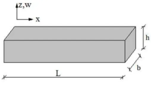
II. MATHEMATICAL MODELLING OF THE PROBLEM Consider an elastic beam of length L , width b, height h, Young's modulus E , and mass density  with uniform cross section A , as shown in Fig. 1.

Fig. 1. Geometry of the beam

Using Euler-Bernoulli beam theory, one can obtain the equation of motion of a beam with homogeneous material properties and constant cross section as follows [1-5]

0 t w x w 2 2 4 4        (1)

where the following definition apply

EI A  

 (2)

here I is the area moment of inertia of the beam cross section, w is the transverse displacement, and t is time.

The solution of the Eq. (2) is sought by separation of variables. Therefore, the displacement is separated into two parts: one is depending on the position and the other is depending on time:

) t ( ) x ( ) t , x (

w   (3)

where  and  are independent of time and position, respectively.

Substituting Eq. (3) into Eq. (2) and after some mathematical rearrangements, the following equation is obtained: 2 2 2 4 4 t ) t ( ) t ( 1 x ) x ( ) x (

1 ___

        

 (4)

Here the each side resulting equation is set to equal a constant, denoted2, to have simple harmonic motion in the beam.

If the position variable of Eq. (4) is separated

0 ) x ( x ) x ( 4 4 4        (5) where    4 2

(6)

If the time variable is separated

0 ) t ( t ) t ( ₂ 2 2        (7)

Eq. (5) is solved as follows:

x cos A x sin A x cosh A x sinh A ) x

(  ₁   ₂   ₃   ₄ 

 (8)

where A₁,A₂,A₃,A₄ are constants, sinh and cosh are the hyperbolic sine and cose functions, respectively.

Eq. (7) is solved as follows:

t cos A t sin A ) t

(  ₅   ₆ 

 (9)

where A5 andA6 are constants.

Thus, if Eq. (8) is multiplied by Eq. (9) to obtainw(x,t), it yields eight combined constants as:







A sin t A cos t



x cos A x sin A x cosh A x sinh A ) t , x ( w 6 5 4 3 2 1             (10) where the constants A₁,A₂,A₃,A₄ can be obtained from the boundary conditions, and A₅,A₆can be obtained from the initial conditions

The boundary conditions satisfied by a C-C, C-F, C-SS, SS-SS beams are as follows, respectively:

0 ) L ( ' w ) L ( w ) 0 ( ' w ) 0 (

w     (11)

0 ) L ( '' ' w ) L ( '' w ) 0 ( ' w ) 0 (

w     (12)

0 ) L ( '' w ) L ( w ) 0 ( ' w ) 0 (

w     (13)

0 ) L ( ' ' w ) L ( w ) 0 ( ' ' w ) 0 (

w     (14)

(3)

obtained for the first ten modes. Finally, using Eq. (6) the natural frequency f_n(Hz) of the beam is found as follows:

  

2

f_n (15)

III. ANNMODELLING OF THE PROBLEM A. Structure of ANN

ANN is a technique that seeks to build an intelligent program using models that simulate the working network of the neurons in the human brain (Fig. 2). Unlike conventional computational programs, the ANN does not have exact data and provides outputs with respect to introduced data set. The data and the circumstances introduced to the program are put into process by the help of various methods of education and learnings. With the aid of the outputs of these transactions, the program assigns weights between the data and the neurotic structures. Afterward, when come up to different situations and data, the cases are commented and results are presented in accordance with previous learnings [32].

Fig. 2. A biologic nerve cell structure

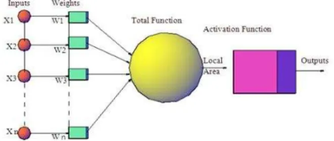
The basic unit of ANN is called as a process element or a node. Although the artificial nerve elements are simpler than the biological nerves, it can simulate the 4 main functions of biological nerves (Fig. 3).

Fig. 3. Artificial neural network sample

There are plenty of neural network models in the existing literature. However, the most preferred neural network model is back propagation model. It is experienced that this model gives pretty good results in the estimation and classification processes [33]. Back propagation neural network is the mostly preferred model because of its capability and excellence to solve problems which are nonlinear and have very complicated structures. Back propagation neural network is a multi-layer and feed-forward neural network trained by the Back Propagation algorithms [7]. This model makes weight assignment processing the inputs and the outputs again and again, and the model tries to minimize the least square errors using this operation. The mathematical expression of this model is as follows [34]

W F b W a

Wn n 1 T _

   

 _ (16)

Here, w is a value of assigned weight between any two neurons, W_n and W_n_₁ are respectively the changes of weightings for n and n-1 values, a is the coefficient of momentum, b_T is the ratio of training, F is the calculated error

where







 

 N

1 i

i i P T N 1

F (17)

here T is the actual output or namely target and i P is the i estimated output value. The working principle of the ANN model is shown in Fig. 4, the inputs are included into the model after weight adjustment. The data are forwarded to the activation function being processed in each neural network with the weights. The results are compared with the actual results in order to determine error. The errors found are transferred to initial weights with the help of Back Propagation and this process is repeated for a number of times which is called as Epoch. Once the process is completed, the results with minimum errors are found [35].

Fig. 4. Neuron weight adjustments

B. Normalizing the data

The input and output values are required to be restricted in some certain rules for artificial neural network models. This process is called as normalization. The most used normalization functions are Min Rule, Max Rule, Median, Sigmoid and Z-Score [32]. In this study, Min-Max normalization rule is applied as below:

min max

min i

Z Z

Z Z ' Z

 

 (18)

Here, Z is the normalized data, ' Z is the actual data, _i max

Z is the maximum data and Zmin is the minimum data. Through this equation, all the data are normalized in the range of [0-1]. Hereby, both the error distribution is done in a narrower range and model runs more quickly.

C. Multiple regression analysis

(4)

the dependent variable [36]. This relationship is expressed as below:

n n 2

2 1

1x b x ... b x b

c

y     (19)

Here, c is a constant number, b are the coefficient of the _i variables.

To calculate the coefficients in the Eq. (19), the mean square method is used. The difference between the actual y and the theoretical y is minimized as follow



1 1i 2 2i n ni



n

1 i

i c B x B x ... B x

y     





(20)

In order to evaluate the accuracy of multiple regression model, the regression coefficient is required to be determined. Besides, multiple regression is applied with respect to Stepwise Selection Method for determining the necessity of the parameters.

IV. RESULTS AND DISCUSSION

In this section, natural frequencies, fn(Hz), of prismatical

steel beams under four different boundary conditions are examined. For this aim, at first natural frequency parameters are obtained, then natural frequencies, f_n(Hz), of prismatical steel beams are found theoretically. Afterward, from obtained these results data sets are constructed. Here, a total of 8640 data sets are used in training stage, and a total of 1920 data sets are used in the testing stage. By this way, 3 main models and a total of 36 sub-models created by changing the number of neurons of the main models. The sizes, moment of inertia and boundary conditions are used as input data parameters. The natural frequency values are employed as outputs. Input data parameters and their intervals and mechanical parameters of steel are given in Table 1 and Table 2, respectively.

TABLE I. THE INPUT DATA PARAMETERS AND THEIR INTERVALS

Parameter Minimum Maximum

b (m) 0.10 0.15

h (m) 0.10 0.15

L(m) 3 3.5

I (m4₎ 6

10 333 .

8   4.219105

n 1 10

Case 1 4

Here, b,h,Land I denote width, height, length and moment of inertia of the beam, and

n

denotes mode number, Case 1,2,3,4 denoted in C-C, C-F, C-SS and SS-SS boundary conditions, respectively.

TABLE II. THE MECHANICAL PARAMETERS OF STEEL

Parameter Description

Young’s Modulus (E) ₂_.₁_₁₀11_N_/_m2 Passion Ratio ( 0.3

Density ( 7850kg/m3

A. Numerical examples

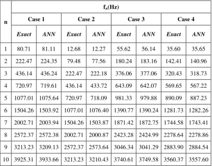
Example 1: In this example, a comparative study is performed to validate the present numerical results. For this purpose, theoretically obtained exact results of natural frequency of the prismatical beams under the four different boundary conditions versus mode number (n) are compared with those obtained using ANN, in Table 3. It is found that the numerical results of both methods are consistent, which show the accuracy of the present ANN model. The absolute errors

are calculated as follows: 100

f f f

nExact nExact

nANN _ _{. Besides, the}

variations of absolute errors in the natural frequencies, f_n(Hz)

, are illustrated in Fig. 5.

TABLE III. VARIATIONS OF NATURAL FREQUENCIES OF THE PRISMATICAL STEEL BEAMS UNDER THE FOUR DIFFERENT BOUNDARY CONDITIONS VERSUS MODE NUMBER (N) (b0.14m;h0.14m;L3m)

n

fn(Hz)

Case 1 Case 2 Case 3 Case 4

Exact ANN Exact ANN Exact ANN Exact ANN

1 80.71 81.11 12.68 12.27 55.62 56.14 35.60 35.65

2 222.47 224.35 79.48 77.56 180.24 183.16 142.41 140.96

3 436.14 436.24 222.47 222.18 376.06 377.06 320.43 318.73

4 720.97 719.61 436.14 433.72 643.09 642.07 569.65 567.22

5 1077.01 1075.64 720.97 718.09 981.33 979.88 890.09 887.23

6 1504.26 1503.92 1077.01 1076.40 1390.77 1390.24 1281.73 1282.26

7 2002.71 2003.94 1504.26 1503.87 1871.42 1872.75 1744.58 1743.41

8 2572.37 2572.38 2002.71 2000.87 2423.28 2424.99 2278.64 2278.86

9 3213.23 3209.13 2572.37 2573.64 3046.34 3041.29 2883.90 2884.54

(5)

Fig. 5. Variations of error in the natural frequencies of the prismatical steel beams under the four different boundary conditions versus mode number (n)

Example 2: Table 4 shows the Model 1, in which 6 inputs, 1 hidden layer and 1 output (see Fig. 6) are used for obtaining the natural frequencies, of the prismatical steel beams under the four different boundary conditions.

Fig. 6. Schematic architecture of Model 1 (6-1-1)

As with all models, feed-forward back propagation algorithm is used in the network type. The tangent and logarithmic sigmoid transfer functions are employed. The number of hidden layer is determined as 1, and 12 separate sub-models are created using the models having 1 to 9 neurons. Actual output values of the natural frequencies are compared with those obtained from training. The results are found with the very small errors, especially for the models with 5 and more neurons.

TABLE IV. TRAINING AND TEST RESULTS FOR MODEL 1

Transfer Function Number of Neurons Training Data Test Data

R² Equation sets MSE % R² Equation sets MSE %

Tan Sig.

1 0.996 y=0.9961x 25.66 0.9913 y=0.9364x 31.23 3 0.9998 y=0.9998x 6.18 0.9933 y=0.938x 12.05 5 1 y=0.9999x 1.80 0.9932 y=0.946x 6.81 7 1 y=0.9999x 1.75 0.9932 y=0.9442x 7.16

8 1 y=x 0.71 0.9931 y=0.9428x 6.71

9 1 y=0.9999x 1.67 0.9929 y=0.9423x 8.04

Log Sig.

1 0.9959 y=0.9964x 25.66 0.9913 y=0.9364x 31.23 3 0.9997 y=0.9997x 8.01 0.9933 y=0.938x 11.40 5 0.9999 y=0.9999x 2.53 0.9932 y=0.946x 7.81 7 0.9999 y=0.9999x 1.68 0.9932 y=0.9442x 7.74 8 0.9999 y=x 0.83 0.9929 y=0.9419x 6.88 9 0.9999 y=0.9999x 1.74 0.9929 y=0.9423x 7.40

To eliminate the possibility of rote learning of these results, 1920 data sets, which are allocated for test, are also included into the model and the obtained results are compared with the exact values. The test data shows that, the interval of error is

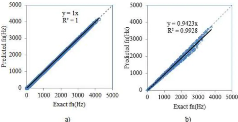
nearly 6-8%, and regression coefficient takes values very close to 1 for the models with 5 and more neurons. In addition, the best agreement is observed in the model with 8 neurons and plotted in Fig. 7.

(6)

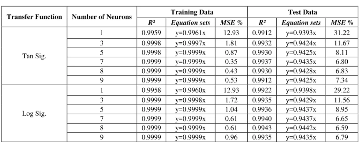
Example 3: Table 5 shows the Model 2, in which 5 inputs, 1 hidden layer and 1 output are used for obtaining the natural frequencies of the prismatical steel beams under the four different boundary conditions. In this model, moments of

inertia, (I), is removed from input parameters and a model with 5 input is created (5-1-1). In the training process of the model for all models of 5 neurons and higher, the error seems to fall below 1%.

TABLE V. TRAINING AND TEST RESULTS FOR MODEL 2

Tan Sig.

1 0.9959 y=0.9961x 12.93 0.9912 y=0.9393x 31.22 3 0.9998 y=0.9997x 1.81 0.9932 y=0.9424x 11.67 5 0.9998 y=0.9999x 0.87 0.9930 y=0.9425x 8.11 7 0.9999 y=0.9999x 0.35 0.9937 y=0.9435x 6.80 8 0.9999 y=0.9999x 0.43 0.9930 y=0.9428x 6.83 9 0.9999 y=0.9999x 0.53 0.9912 y=0.9425x 7.34

Log Sig.

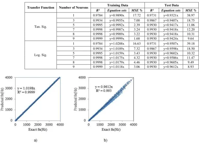
Considering the errors, the model for logarithmic sigmoid transfer function with 8 neurons is found the best and illustrated in Fig. 8.

It should be noted that, although having one missing input parameter in comparison with the Model 1, the present model does not show serious differences in error rates for both training and test results.

Fig. 8. Scatter diagrams of Model 2 for logarithmic sigmoid transfer function with 8 neurons a) training b) test

Example 4: Table 6 shows the Model 3. Here parameters are tried to be identified with numbers from 1 to 10 instead of calculations of frequency parameter value. Therefore, the natural frequency parameters are aimed to be determined with ANN model without any calculation in advance. As the model results are examined, it is found that the results are worse than the results of previous ANN models in terms of both training and test. However, in other models, either moment of inertia or natural frequency parameters are included into the model with pre-calculating.

For this model, all the inputs are introduced to the model with simple numeric expressions and the outputs are obtained. As a result, the errors are found very minimal as being 8.93% for the test of the model for logarithmic sigmoid transfer function with 9 neurons and plotted in Fig. 9.

Example 5: Table 7 shows Model 4, in which the training inputs are implanted to the model step by step and adjusted

2

R values are investigated. The step in which the adjusted R2 values decrease or remain constant; the included parameters are excluded from the model.

According to the steps of the process of Table 7, the input of moment of inertia is excluded and a multiple regression model is constructed with the remaining 5 input parameters in Table 8.

(7)

TABLE VI. TRAINING AND TEST RESULTS FOR MODEL 3

Tan. Sig.

Log. Sig.

Fig. 9. Scatter diagrams of Model 3 for logarithmic sigmoid transfer function with 9 neurons a) Training b) Test

TABLE VII. ADJUSTED R² ANALYSIS RESULTS

Model R R2_{Adjusted R}2 _{Std. Error of the Estimate}

1 0.966 0.932 0.932 259.46804

TABLE VIII. MULTIPLE REGRESSION ANALYSIS RESULTS

Unstandardized Coefficients

Standardized Coefficients

95.0% Confidence Interval for B

B Std. Error Beta Lower Bound Upper Bound Constant -728.779 106.944 -938.414 -519.144

Case -2.113 2.498 -0.002 -7.010 2.783

B 0.100 163.450 0.000 -163.350 163.550

H 9238.788 163.450 0.158 8918.388 9559.188

(8)

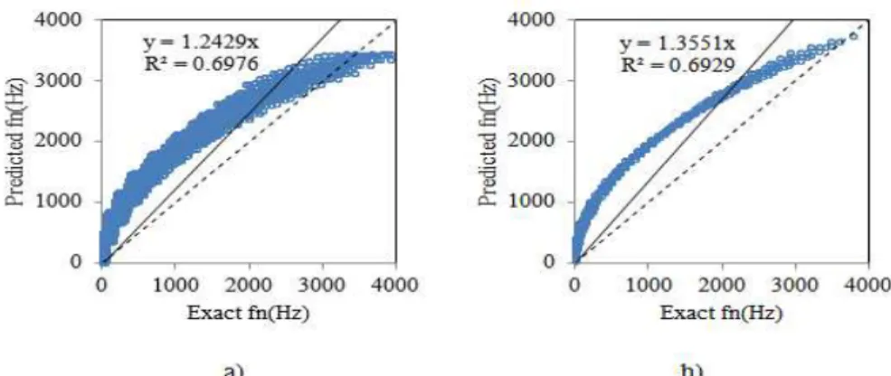
Fig. 10.Scatter diagrams of multiple regression model a) Training b) Test

V. CONCLUSION

In this study, bending natural frequencies of the prismatical steel beams with various geometrical characteristics under the four different boundary conditions are determined using ANN technique. In that way, an alternative efficient method is aimed to develop for the solution of the existing problem, which provides avoiding loss of time for computing some necessary parameters.

Briefly the following results are obtained:

1) The tangent sigmoid transfer function shows better performance in Model 1 with 8 neurons

2) The logarithmic sigmoid transfer function shows better performance in Model 2 with 8 neurons

3) When the first two models are considered it is concluded that ANN models do not need moment of inertia parameter in the training

4) The logarithmic sigmoid transfer function provides better results in Model 3 with 9 neurons

5) It is found from Model 4 that the moment of inertia has not any efficiency. This finding also supports the results found by the Models 1 and 2

6) The errors of the models having 5 or more neurons are lower, and this prove at least 5 neurons should be used for the reliably of the model

7) The two transfer functions have quite similar errors, and so both of them can be used

8) The constructed ANN models give more efficient results than the multiple regression model

REFERENCES

[1] S. P. Timoshenko, Vibration Problems in Engineering, D. Van Nostrand, Princeton, NJ, 1937.

[2] E. B. Magrab, Vibration of Elastic Structural Members, Netherlands, Sijthoff and Noordhoff, 1979.

[3] A. W. Leissa and M. S. Qatu Vibration of Continuous Systems, McGraw Hill Companies, 2011.

[4] S. S. Rao, Vibration of Continuous Systems, John Wiley & Sons, Inc., Hooken, New Jersey, 2007.

[5] C. Y. Wang and C. M. Wang, Structural Vibration: Exact Solutions for Strings, Membranes, Beams and Plates, CRC Press, Taylor and Francis Group, Boca Raton, 2014.

[6] J. C. Hsieh and R. H. “Plaut, Free vibrations of inflatable dams,” Acta Mech. 1990; vol. 85: pp. 207-220.

[7] M. C. Ece, M. Aydogdu and V. Taskin, “Vibration of a variable cross-section beam” Mech Res Commun. 2007, vol. 34, pp. 78-84.

[8] M. Şimşek, and T. Kocatürk, “Free vibration analysis of beams by using a third order shear deformation theory,” Sadhana Acad Proc Eng Sci. 2007, vol. 32, pp. 167-179.

[9] Ö. Civalek, “Free vibration analysis of symmetrically laminated composite plates with first-order shear deformation theory (FSDT), by discrete singular convolution method,” Finite Elem Anal Des. 2008, vol. 44, pp. 725-731.

[10] Ö. Civalek and M. Gürses, “Free vibration analysis of rotating cylindrical shells using discrete singular convolution technique,” Int J Pres Ves Pip. 2009, vol. 86, pp. 677-683.

[11] M. Avcar, “Free vibration of randomly and continuously non- homogenous beams with clamped edges resting on elastic foundation,” J Eng Sci Des. 2010, vol.1, pp. 33-38 (in Turkish).

[12] B. Akgöz and Ö. Civalek, “Longitudinal vibration analysis of strain gradient bars made of functionally graded materials,” Compos B Eng. 2013, vol. 55, pp. 263-268. ·

[13] M. Avcar, “Free vibration analysis of beams considering different geometric characteristics and boundary condition,” Int. Appl. Mech. 2014, vol.4, pp. 94-100.

[14] A. Prokic, M. Besevic and D. Lukic, “A numerical method for free vibration analysis of beams,” Lat Am J Solid Struct. 2014, vol. 11, pp. 1432-1444.

[15] Y. Yeşilce, “Differential transform method and numerical assembly technique for free vibration analysis of the axial-loaded Timoshenko multiple-step beam carrying a number of intermediate lumped masses and rotary inertias,” Struct Eng Mech. 2015, vol. 53, pp. 537-573 [16] L. A. Zadeh, “Fuzzy logic, neural networks and soft computing,”

Commun ACM. 1994, vol. 37, pp. 77-84.

[17] S. K. Das, A. Kumar, B. Das and A. P. Burnwal, “On soft computing techniques in various areas,” Int J Inform Tech Comput Sci, 2013, vol. 3, pp, 59-68.

[18] H. Adeli, "Neural networks in civil engineering: 1989−2000,” Comput Aided Civ Infrastruct Eng. 2001, vol. 16, pp. 126–142.

[19] R. Gates, M. Choi, S. K. Biswas and J.J. Helferty, “Stabilization of flexible structures using artificial neural networks,” Proc Int Joint Conf Neural Network. 1993, vol. 2, pp. 1817-1820.

[20] B. Karlik, E. Özkaya, S. Aydin and M Pakdemirli, “Vibrations of a beam-mass systems using artificial neural networks,” Comput. Struct. 1998, vol. 69, pp. 339-347.

[21] M. A. Mahmoud and M. A. A. Kiefa, “Neural network solution of the inverse vibration problem,” NDT E Int. 1999, vol. 32, pp. 91-99. [22] E. Castillo, A. Cobo, J. M. Gutierrez and E. Pruneda, “Functional

networks: A new network–based methodology,” Comput Aided Civ Infrastruct Eng.2000, vol. 15, pp. 90–106.

(9)

[24] Ö. Civalek, “Flexural and axial vibration analysis of beams with different support conditions using artificial neural networks,” Struct Eng Mech. 2004, vol. 18, pp. 303-314.

[25] A. P. Hassanpour, E. Esmailzadeh and H. Mehdigholi, “Vibration of beams with unconventional boundary conditions using artificial neural network,” Proc ASME Int Des Eng Tech Conf Comput Inf Eng. 2005, vol. 1, pp. 159-165.

[26] S. M. Bagdatli, E. Özkaya, H. A. Özyiğit and A. Tekin, “Nonlinear vibrations of stepped beam systems using artificial neural networks,” Struct Eng Mech. 2009, vol. 33, pp. 15-30.

[27] R. A.. Saeed, A. N. Galybin and V. Popov. "Crack identification in curvilinear beams by using ANN and ANFIS based on natural frequencies and frequency response functions," Neural Comput. Appl. 2012, vol. 21 pp. 1629-1645.

[28] N. A. Jalil and I. Z. M. Darus, “Non-parametric Neuro-Model of a Flexible Beam Structure” IEEE Symp Comp Inf (ISCI), Langkawi, Malaysia, 2013, pp. 45-50.

[29] M. Mohammadhassani, H. Nezamabadi-pour, M. Suhatril and M. Shariati, “Identification of a suitable ANN architecture in predicting strain in tie section of concrete deep beams” Struct Eng Mech. 2013, vol. 46, pp. 853-868.

[30] Z. C. Ding, M. S. Cao, H. L. Jia, L. X. Pan and H. Xu “Structural dynamics-guided hierarchical neural-networks scheme for locating and quantifying damage in beam-type structures." J Vibroeng. 2014, vol. 16, pp. 3595-3608.

[31] M. Karimi, A. Shooshtaria and S. Razavia, “Large amplitude vibration prediction of rectangular plates by an optimal artificial neural network (ANN),” J Comput Appl Res Mech Eng. 2014, vol.4, pp. 55-65. [32] Z. Şen, Principles of Artificial Neural Networks, Turkish Water

Foundation Publications, 2004 (in Turkish).

[33] Ç. Elmas, Artificial Neural Networks (Theory, Architecture, Education, Application), Ankara: Seçkin Publication House, 2003 (in Turkish). [34] S. Rajasekaran and G. Pai, Neural Networks, Fuzzy Logic And Genetic

Algorithms, Synthesis & Applications. New Delh: Prentice-Hall of India Private Limited, 2003.

[35] M. M. Alshihri, A. M. Azmy and M. S. El-Bisy, “Neural networks for predicting compressive strength of structural light weight concrete,” Construct. Build. Mater. 2009, vol. 23, pp. 2214–2219.