www.hydrol-earth-syst-sci.net/16/983/2012/ doi:10.5194/hess-16-983-2012
© Author(s) 2012. CC Attribution 3.0 License.
Earth System
Sciences
Selecting the optimal method to calculate daily global reference
potential evaporation from CFSR reanalysis data for application in
a hydrological model study
F. C. Sperna Weiland1,2, C. Tisseuil3, H. H. D ¨urr1, M. Vrac4, and L. P. H. van Beek1
1Department of Physical Geography, Utrecht University, P.O. Box 80115, 3508 TC, Utrecht, The Netherlands 2Deltares, P.O. Box 177, 2600 MH, Delft, The Netherlands
3Mus´eum National d’Histoire Naturelle, UMR BOREA-IRD 207/CNRS 7208/MNHN/UPMC, D´epartement Milieux et Peuplements Aquatiques, Paris, France
4Laboratoire des Sciences du Climat et de l’Environnement (LSCE-IPSL) CNRS/CEA/UVSQ, Centre d’´etude de Saclay, Orme des Merisiers, 91191 Gif-sur-Yvette Cedex, France
Correspondence to:F. C. Sperna Weiland ([email protected])
Received: 1 July 2011 – Published in Hydrol. Earth Syst. Sci. Discuss.: 28 July 2011 Revised: 15 March 2012 – Accepted: 16 March 2012 – Published: 27 March 2012
Abstract. Potential evaporation (PET) is one of the main inputs of hydrological models. Yet, there is limited consen-sus on which PET equation is most applicable in hydrolog-ical climate impact assessments. In this study six different methods to derive global scale reference PET daily time se-ries from Climate Forecast System Reanalysis (CFSR) data are compared: Penman-Monteith, Priestley-Taylor and origi-nal and re-calibrated versions of the Hargreaves and Blaney-Criddle method. The calculated PET time series are (1) eval-uated against global monthly Penman-Monteith PET time se-ries calculated from CRU data and (2) tested on their usabil-ity for modeling of global discharge cycles.
A major finding is that for part of the investigated basins the selection of a PET method may have only a minor in-fluence on the resulting river flow. Within the hydrological model used in this study the bias related to the PET method tends to decrease while going from PET, AET and runoff to discharge calculations. However, the performance of indi-vidual PET methods appears to be spatially variable, which stresses the necessity to select the most accurate and spa-tially stable PET method. The lowest root mean squared differences and the least significant deviations (95 % signifi-cance level) between monthly CFSR derived PET time series and CRU derived PET were obtained for a cell-specific re-calibrated Blaney-Criddle equation. However, results show that this re-calibrated form is likely to be unstable under changing climate conditions and less reliable for the calcu-lation of daily time series. Although often recommended, the Penman-Monteith equation applied to the CFSR data did not outperform the other methods in a evaluation against PET
derived with the Penman-Monteith equation from CRU data. In arid regions (e.g. Sahara, central Australia, US deserts), the equation resulted in relatively low PET values and, con-sequently, led to relatively high discharge values for dry basins (e.g. Orange, Murray and Zambezi). Furthermore, the Penman-Monteith equation has a high data demand and the equation is sensitive to input data inaccuracy. Therefore, we recommend the re-calibrated form of the Hargreaves equa-tion which globally gave reference PET values comparable to CRU derived values for multiple climate conditions.
The resulting gridded daily PET time series provide a new reference dataset that can be used for future hydrological impact assessments in further research, or more specifically, for the statistical downscaling of daily PET derived from raw GCM data. The dataset can be downloaded from http://opendap.deltares.nl/thredds/dodsC/ opendap/deltares/FEWS-IPCC.
1 Introduction
and actual evapotranspiration (AET; for list of abbreviations see Table 1) are seldomly monitored and General Circulation Model (GCM) datasets, employed for future impact assess-ments (Sperna Weiland et al., 2012b), often lack AET data (PCMDI, 2010).
Here, we prefer to calculate potential evaporation (PET) from GCM data and to derive AET within a hydrological model over using GCM AET directly. This because within global hydrological models (GHMs), AET is calculated on a higher grid resolution and processes related to transpira-tion and soil moisture are modeled with a water balance in-stead of energy balance approach which at least guarantees that negative evaporation does not occur (Sperna Weiland et al., 2012a). In addition, GCM AET is often biased due to, amongst others, biases in PR, radiation and soil moisture availability (Mahanama and Koster, 2005; Elshamy et al., 2009; Sperna Weiland et al., 2012a). Of course, it should be noted here that off-line calculation of PET and AET can also be biased by deviations in GCM radiation used as input for some of the PET equations or through interaction between the different atmospheric variables within the GCM.
Within hydrological model studies monthly PET time-series, or monthly PET time-series downscaled to daily val-ues (for example based on temperature), have frequently been used (Van Beek, 2008; Sperna Weiland et al., 2010; Arnell, 2011). Currently, most hydrological models run on a daily or smaller time-step, as most hydrological processes show a high variability over time. Consequently, these mod-els can also benefit from daily PET time-series as model in-put. In addition, the input data of PET equations is now often provided on a daily time step. Therefore, this study focuses on calculation of daily PET time series using daily values of the required atmospheric variables. A historical global gridded PET time series will be created that can be used as reference for the statistical downscaling of daily GCM data. Downscaling of PET time series was preferred over down-scaling of the individual GCM input variables of the PET equation, since by individual downscaling inconsistencies between the atmospheric input variables can be introduced (Piani et al., 2010).
For the creation of these PET time series a consistent observational dataset of current climatic conditions at high spatial and temporal resolution is needed. Here we used the recently developed Climate Forecast System Reanalysis (CFSR) dataset (Saha et al., 2006, 2010) which is of partic-ular interest for three major reasons. Firstly, it is a data set with a high spatial (∼0.3◦× ∼0.3◦) and temporal (6-hourly)
resolution covering the entire globe. Secondly, in the short term, the CFSR dataset is likely to supersede its predecessor, the widely known US NCEP/NCAR (National Center for En-vironmental Prediction/National Center for Atmospheric Re-search) reanalysis data (Kalnay et al., 1996). And thirdly, the CFSR dataset contains all required atmospheric fields to cal-culate and compare a range of PET equations.
Table 1.Abbreviations.
Abbreviaton Long name/description
AET Actual evapotranspiration
BC Blaney-Criddle
BCorig Original Blaney-Criddle equation BCrecal Re-calibrated Blaney-Criddle equation CDF Cumulative distribution function CFSR Climate forecast system reanalysis
CFSR PET Potential evaporation calculated from CFSR data CFSR PM PET Penman-Monteith potential evaporation from CFSR data CRU Climate research unit, University of East Anglia
CRU TS 2.1 1901–96 Monthly Grids of Terrestrial Surface Climate, CRU CRU CL 1.0 1961-90 mean monthly terrestrial climatology, CRU CRU PET Potential evaporation calculated from CRU data CRU PM PET Penman-Monteith potential evaporation from CRU data CV Coefficient of variation
DJF December, January, February
FAO United Nations Food and Agriculture Organization GCM General circulation model / global climate model GHM Global hydrological model
GLCC Global Land Cover Characterization GRDC Global runoff data centre HG Hargreaves equation HGorig Original Hargreaves equation HGrecal Re-calibrated Hargreaves equation HGPET Hargreaves potential evaporation JJA June, July, August
MAM March, April, May
NCAR National Center for Atmospheric Research NCEP National Centre for Environmental Prediction PCR-GLOBWB PCRaster code global water balance model PET Potential evaporation
PM Penman-Monteith
PR Precipitation
PT Priestley-Taylor QC (Channel) discharge QL Cell specific runoff RMSD Root mean squared difference SON September, October, November
US United States
The equation is applicable in a variety of climatic condi-tions and shows overall good agreement with the PM method (Droogers and Allen, 2002). Several studies highlighted sig-nificant improvement of the HG equation by increasing its multiplication factor (Droogers and Allen, 2002). This will be tested here as well.
The more empirical BC equation depends on less input variables and may therefore be less sensitive to GCM and re-analysis data quality (Kingston et al., 2009; Weiß and Men-zel, 2008; Lu et al., 2005). With the temperature-based BC equation the computation time required for both calculation of PET and downscaling of the required input variables can be reduced, while the method provides results comparable to other PET methods (Oudin et al., 2005; Blaney and Criddle, 1950). Yet, Jensen (1966) showed that the climate depen-dency of the BC equation disables its application in multiple different climate zones. To overcome this problem we tested the local-recalibrated BC method proposed by Ekstr¨om et al. (2007).
The main goal of this study is the construction of a global gridded dataset of reference PET at high spatial (0.5 degree) and temporal (daily) resolution from CFSR reanalysis data using one of the following six PET equations; PM, HG, PT, BC and the HGrecal and BCrecal equations. The constructed daily PET dataset will be validated annually and seasonally for the period 1979–2002 against the Climate Research Unit (CRU) dataset (CRU TS 2.1 and CRU CL 1.0) which is often considered as a standard (Mitchell and Jones, 2005; New et al., 2000, 1999; Droogers and Allen, 2002; IPCC, 2007). In a first step, a sensitivity analysis of the influence of the differ-ences between individual CFSR and CRU atmospheric vari-ables on calculated PET is given. In a final step, the transfer of differences between the six PET methods throughout the hydrological modeling chain (i.e. from PET to AET to runoff and discharge) will be assessed by inter-method comparison and the goodness-of-fit between modeled and observed river discharge.
2 Data and methods
2.1 CFSR reanalysis data
The CFSR dataset is a reanalysis product which is developed as part of the Climate Forecast System (Saha et al., 2006, 2010) at the National Centers for Environmental Prediction (NCEP). The CFSR dataset became available in 2010 and su-persedes the previous NCEP/NCAR reanalysis dataset which has been widely used in downscaling studies (e.g. Michelan-geli et al., 2009; Maurer et al., 2010; Wilby et al., 1998). At this stage the CFSR dataset spans the period 1979 to present and has a resolution of approximately 0.25 degrees around the equator to 0.5 degrees beyond the tropics (Higgins et al., 2010). In this study, 6-hourly temperature, radiation, air pressure and wind data were averaged to a daily time-step for
the period 1979–2002. These daily time series were then in-terpolated to the regular 0.5 degrees PCR-GLOBWB model grid using bilinear interpolation.
2.2 CRU reference potential evaporation
For validation reference historical PET time series were calculated from the CRU datasets with the by the United Nations Food and Agriculture Organization (FAO) recom-mended PM equation (Monteith, 1965; Allen et al., 1998). Temperature, vapor pressure and cloud cover were retrieved from the CRU TS2.1 monthly time series (New et al., 2000). Wind speed was obtained from the monthly climatology, CRU CL 1.0 (New et al., 1999) because monthly CRU TS2.1 time series are not provided for this variable. Diffusiv-ity, i.e. the effectiveness by which heat and vapour can be exchanged with the atmosphere, was calculated following Allen et al. (1998). As radiation is not included in the CRU datasets, a standard climatological maximum radiation cycle was calculated using the day-number and latitude as input (Allen et al., 1998). This maximum radiation was reduced to incoming radiation at the surface with monthly CRU cloud cover time-series. The resulting monthly PET time series, which are here used as reference for the validation of the CFSR derived PET, are subject to uncertainties as well due to biases in and availability of the meteorological input data and due to simplifications in the equation. Yet, to our opin-ion they form one of the best available global reference PET dataset (Mitchell and Jones, 2005; Droogers and Allen, 2002; IPCC, 2007). For application in the hydrological model the CRU time-series have been downscaled to daily values using the monthly PR and temperature quantities from the CRU datasets and the daily distribution of these variables from the CFSR dataset following Van Beek et al. (2008). It should be noted that the measurement based CRU dataset is sub-ject to inaccuracies as well. In addition, the data from the CRU CL 1.0 climatology is derived from data for the period 1961 to1990 and has been used for the calculation of PET for the period 1990 to 2002 as well. This may have introduced inconsistencies due to meteorological changes over the past decades. The influence of these inconsistencies is minimized by analyzing long-term average PET results only.
2.3 Potential evaporation equations
Within this study we compare daily CFSR PET time series derived with six different PET equations. The equations considered are: (1) the physically based PM equation, (2) the radiation and temperature-based PT equation, (3) the HG equation which requires as input time-varying temperature and extra-terrestrial radiation, (4) the empirical temperature-based BC equation and additional modified forms of the (5) HG and (6) BC equations (Table 2).
Table 2.Potential evaporation equations.
Method Acronym Equation Reference
Penman-Monteith PM ET0=
1(Rn−G)+ρacp(es−raea )
λv1+γ (1+rrs a)
Monteith (1965)
Hargreaves HGorig ET0= 0.0023·Ra·(T+17.8)·TR0.50 Hargreaves and Samani (1985) Modified Hargreaves HGrecal ET0= 0.0031·Ra·(T+17.8)·TR0.50 This study
Priestley-Taylor PT ET0=αλv1R(1+nγ ) Priestley and Taylor (1972)
Blaney-Criddle BCorig ET0=p(0.46T+8) Blaney and Criddle (1950)
recalibrated Blaney-Criddle BCrecal ET0=p(aT+b) Ekstr¨om et al. (2007)
λv= latent heat of vaporization (J/g),1= the slope of the saturation vapour pressure temperature relationship (Pa K−1),R
n= net radiation (W m−2),G= Soil heat flux (W m−2), cp= specific heat of the air (J kg−1K−1),ρa= mean air density at constant pressure (kg m−3),es−ea= vapor pressure deficit (Pa),rs= surface resistances (m s−1),ra= aerodynamic resistances (m s−1),γ= psychrometric constant (66 Pa K−1),R
a= extraterrestrial radiation (MJ m−2day−1),T= mean daily temperature (◦C), TR = temperature range (◦C),
α= empirical multiplier (–; 1.26),p= mean daily percentage of annual daytime hours (%),aandbare the coefficients of the Blaney-Criddle equation which are adjusted to cell specific values in the recalibration.
al. (2007). In this modified BC equation, the multiplica-tive and addimultiplica-tive coefficients (e.g. 0.46 and 8) have been re-calibrated to cell-specific values (see the resulting coefficient values in Fig. 1). This was done by linearly regressing the cell specific long-term average mean monthly CFSR temper-ature to the CRU derived long-term average monthly PET for the complete period with overlapping data available for the two datasets (1979–2002). The slopes and intercepts of this linear regression exercise were used to calculate the coeffi-cient values. For the empirical BC equation, which consid-ers only limited meteorological variables, a cell specific re-calibration was preferred (this is also illustrated by the large spatial variation in bias between BC PET derived from CFSR data and reference PM PET derived from CRU data, as will be presented in the results section).
The HG equation was also applied in its original form (HGorig) and in a re-calibrated form (HGrecal). The HG equation is recognized as an efficient empirical equation with low input data demand, while it integrates consistent infor-mation on the spatial variability of climate conditions such as the daily temperature range and a spatial radiation pattern. The spatial radiation pattern is defined as a fixed annual cycle with a daily time-step where values vary with latitude and ju-lian day number (Allen, 1998). Preliminary results indicated that the PET time series derived from the CFSR dataset us-ing the original HG (HGorig) equation gave an overall global underestimation of CRU PET (as will be shown in the results section) with little spatial variability. Therefore, instead of a cell-specific re-calibration, we applied a global uniform modification to the HG equation, by increasing uniformly the multiplication factor in the equation for all grid cells from 0.0023 to 0.0031. Similar increases were proposed by Allen (1993) and Droogers and Allen (2002). To determine the optimal value of the multiplication factor the long term average monthly CFSR HGorig time series were linearly fit-ted against CRU PET. The multiplication factor was then var-ied with intervals of 0.0001 until the lowest global average
a.
b.
Fig. 1. Cell specific values of the coefficients in the re-calibrated Blaney-Criddle equation. The values in(a)replace the number 0.46 and the values in(b)replace the number 8 in the original Blaney-Criddle equation (ET0=p(0.46T+ 8)).
root mean squared difference (RMSD) value was obtained for the monthly average PET time series.
2.4 Global hydrological modelling
Each model cell, with a resolution of 0.5 degrees, consists of two vertical soil layers and one underlying groundwater reservoir. Sub-grid parameterization is used for the schema-tization of surface water, short and tall vegetation and for calculation of saturated areas for surface runoff as well as in-terflow. Water enters the cell as rainfall and can be stored as canopy interception or snow. Snow is accumulated when temperature is below 0◦
C and melts when temperature is higher. Melt water and throughfall are passed to the sur-face, where they either infiltrate in the soil or become surface runoff. Exchange of soil water is possible between the soil and groundwater layers in both up- and downward direction, depending on soil moisture status and groundwater storage. Total runoff consists of non-infiltrating melt water, saturation excess surface runoff, interflow and base flow.
Time series of reference PET are prescribed to the hydro-logical model and converted to AET internally. Reference potential evapotranspiration is converted into crop-specific potential evapotranspiration using a crop factor (Allen et al., 1998). PCR-GLOBWB distinguishes two land cover types, short and tall vegetation, given the distinctive differences in plant height, canopy cover and root distributions. The aggre-gation of different vegetation types into two land cover types is expedient from a computation point of view. However, by basing the parameterization of the different land cover types on the Global Land Cover Characterization (GLCC 2; Loveland et al., 2000) database which has a resolution of 30 arc seconds, much of the sub-grid variability in vegeta-tion condivegeta-tions can be preserved at the 0.5 degree resoluvegeta-tion. Also, although the imposed potential evapotranspiration is called crop-specific, it should be noted that this concerns both natural and cultivated areas. To account for seasonal variations in the crop-specific evaptranspiration, the crop fac-tor is represented by a monthly climatology that reflects the phenology and in case of cultivated surfaces, also the crop calendar.
Crop-specific potential evapotranspiration needs to be par-titioned into two fluxes, one through the soil matrix (bare soil evaporation) and one through the roots and stomata of vege-tation (transpiration). Since vegevege-tation stands are layered and ground cover variable, a break-down on the basis of the min-imum crop factor and that of the stand as a whole is preferred over one on the basis of cover fraction. Adopting the upper value for the minimum crop factor (0.2, Allen et al., 1998), the potential evaporation and transpiration flux become:
ES0=ksPET (1)
T0=kcPET (2)
where PET is reference PET (m day−1),k
sis the “crop fac-tor” used for bare soil, ES0 is potential bare soil evapora-tion (m day−1),k
c is the monthly crop factor andT0is po-tential crop specific transpiration (m day−1). The aggrega-tion of crop types to two vegetaaggrega-tion classes on a grid with
a resolution of 0.5 degrees is a simplification of real world vegetation and will in the end impact calculated PET fields.
Potential bare soil evaporation and plant transpiration are reduced to AET based on soil moisture conditions. As sub-grid variation in soil water storage capacity is considered, part of the surface area may be saturated (Improved Arno Scheme; Hagemann and Gates, 2003). Over this saturated area, potential bare soil evaporation can be sustained as long as the rate does not exceed the saturated hydraulic conductiv-ity. Similarly, over the fraction of the cell where the surface remains unsaturated, the rate is limited by the unsaturated hy-draulic conductivity. In the case of transpiration, no transpi-ration can occur over the saturated part due to oxygen stress, while over the unsaturated area the rate diminishes between full to no transpiration from field capacity to wilting point as a result of water stress. Bare soil evaporation is capable of exhausting soil moisture in the upper soil layer of the model only, whereas transpiration can draw from both layers given the root distribution.
For each daily time-step the water balance, and its result-ing runoff and AET fluxes, are computed for all model cells. The cell specific runoff is accumulated and routed as river discharge along the drainage network taken from the global Drainage Direction Map (DDM30; D¨oll and Lehner, 2002) using the kinematic wave approximation of the Saint-Venant equation. Due to the coarse resolution of this large scale hy-drological model, river discharge can only reliably be calcu-lated for large river basins.
2.5 Statistical validation
The six PET time series derived from CFRS data were val-idated for the period 1979 to 2002 against monthly CRU based PM PET time series (CRUPM) and compared with each other, using six statistical quantities:
1. A first simple comparison was made by calculating global maps with biases in long-term average annual means:
BIAS=PETCFSR−PETCRU (3)
that the method is not reliable when applied to the se-lected global datasets. As a consequence, the CFSR derived AET and runoff maps are only validated by a comparison between methods.
2. To illustrate the significance of the biases calculated in step one, global significance maps have been calculated for PET, AET and local runoff independently. Hereto the significance of the differences between annual av-erage CRU and CFSR derived time series have been quantified with the Welch’s t-test (Welch, 1947) for a significance level of 95 %. The Welch’s adaptation of the standard student’s t-test is used when the two sam-ples possibly have unequal variances.
t=XCRU−XCFSR r
s2 CRU
nCRU+
s2 CFSR
nCFSR
(4)
WhereXCRUis the long-term annual average PET, AET or runoff value calculated from the CRU dataset and XCFSRis the long-term annual average calculated from the CFSR dataset for one of the six equations, SCRU is the standard deviation CRU derived annual average PET, AET or runoff values (for all variables 24 annual values over the period 1979 to 2002) andSCFSRis the standard deviation of the 24 CFSR derived annual av-erage values,nCFSR andnCFSR are the number (24) of annual average values for both datasets.
3. To analyze the seasonal varying character of the bi-ases, global maps with cell specific RMSD (m day−1) of the monthly time series (Eq. 5) have been created. These maps give an indication of regional performance on the smallest time-scale at which the validation data is available: RMSD= v u u u t N P
i=1
(PETCRUi−PETCFSRi)2
N (5)
where PETCFSR refers to the monthly PET calculated from the CFSR data set, PETCRUrefers to the monthly PM-based PET calculated from the CRU dataset, i is the month number andNis the total number of months (N= 288).
4. Global maps with long-term annual and seasonal aver-age PET, AET and runoff have been calculated to il-lustrate the differences between methods while moving through the hydrological model chain.
5. To quantify the variation between the six different equa-tions, cell specific values of the coefficient of variation
(CV) have been calculated from long-term average PET maps calculated with the six different PET equations:
CV=
M
P
j=1
s
1 K
K
P
k=1
(PETk,j−PETj)2
PETj
M (6)
Where PETj is the average of PET calculated with the
6 equations for the specific cellj. PETk,j is the PET
calculated for thekth equation for cellj,Kis the total number of equations (6),Mis the total number of grid cells.
In addition, global average CV values have been calcu-lated for PET, AET, runoff and discharge and basin spe-cific CV values have been calculated from the annual average river discharge.
6. Performance of the different methods for the reproduc-tion of correct AET amounts is more explicitly evalu-ated by comparing long-term average modeled river dis-charge with disdis-charge observations. To this end, annual average discharge is modeled with PCR-GLOBWB forced with temperature, PR and PET from the CFSR dataset for a selection of 19 large rivers (Sperna Weiland et al., 2010). For validation, observed discharge was obtained from the Global Runoff Data Centre (GRDC; GRDC, 2007). The data was adjusted by adding an esti-mation of water use (Wada et al., 2010; Sperna Weiland et al., 2010).
3 Results
3.1 Impact of differences in individual meteorological variables from the CFSR and CRU datasets on PM PET
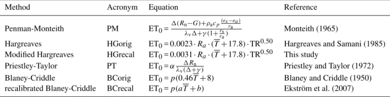
Global maps with the bias of monthly CFSR-CRU derived PM PET from daily CFSR PM PET are shown for all four seasons in Fig. 2. Within all these maps PET is calculated with the PM equation. Yet, in the top row the daily average CFSR data is replaced by monthly averages in the calculation of PM PET. The maps show that there is limited difference in seasonal averages when using either CFSR daily or CFSR monthly average values as input to the PM equation (Fig. 2a). Therefore, the CFSR PET time-series can be evaluated on a monthly time-scale with CRU data.
CFSR monthly DJF CFSR monthly MAM CFSR monthly JJA CFSR monthly SON
CFSR CRU tmp DJF CFSR CRU tmp MAM CFSR CRU tmp JJA CFSR CRU tmp SON
CFSR CRU rad DJF CFSR CRU rad MAM CFSR CRU rad JJA CFSR CRU rad SON
CFSR CRU wnd DJF CFSR CRU wnd MAM CFSR CRU wnd JJA CFSR CRU wnd SON
CFSR CRU vap DJF CFSR CRU vap MAM CFSR CRU vap JJA CFSR CRU vap SON
d. b.
c.
e.
f.
Fig. 2. Global maps with bias of monthly CFSR-CRU derived Penman-Monteith potential evaporation (m day−1) from daily Penman-Monteith potential evaporation calculated from the daily CFSR time-series for all four seasons. From top to bottom: bias for(b)the full CFSR dataset where al input variables are aggregated to a monthly time-step,(c)the CFSR datasets aggregated to monthly values and temperature replaced with CRU TS2.1 values,(d)the CFSR datasets aggregated to monthly values and incoming radiation derived from an annual sinusoidal radiation cycle and the CRU TS2.1 cloud cover,(e)the CFSR datasets aggregated to monthly values and wind from the CRU CL 1.0 dataset,(f)the CFSR datasets aggregated to monthly values and vapor pressure from the CRU TS2.1 time-series.
radiation cycle reduced with the CRU TS2.1 cloud clover, larger alterations are introduced in the PET fields (Fig. 2c). PET becomes higher over summer in arid regions and lower in humid regions, as for example southern-America and par-ticularly the Amazon. The influence of using a climatologi-cal cycle for windspeed is also quite pronounced (Fig. 2d) as could be expexted according to (Roderick et al., 2007). With the CRU climatological wind data PET is overall reduced in the SON and DJF seasons over most of the Southern Hemi-sphere and in the JJA season over the Northern HemiHemi-sphere. Particularly in the MAM and JJA season, PET increases over the Sahara when using climatiological wind fields.
Finally, replacing the vapor pressure obtained from the CFSR dataset (which is calculated from an approximiation using the minimum air temperature for the dew-point tem-perature; Allen et al., 1998; Sperna Weiland et al., 2010) with the CRU TS2.1 vapor pressure fields does not alter the global pattern a lot (Fig. 2e). Yet, locally, in the Sahara and other desert regions in for example Australia and the south-western US, high PET values are reduced.
Overall it can be concluded that especially the difference introduced by using climatological radiation and wind in-stead of their CFSR equivalents is large. Differences intro-duced by using the CRU temperature are smaller, the differ-ence introduced by using CRU vapor pressure is negligible.
3.2 Evaluation of global potential evaporation
3.2.1 Long-term average annual bias
a) PM d) PT
b) HGorig e) HGrecal
c) BCorig f) BCrecal
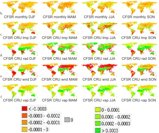
Fig. 3.Global maps with annual average bias of CFSR estimated daily reference potential evaporation (PET; m day−1)from annual average CRU Penman-Monteith reference PET. In the left column bias in PET obtained with the Penman-Monteith (PM), the standard Hargreaves (HGorig) and Blaney-Criddle (BCorig) method are displayed. In the right column bias obtained with Priestley-Taylor (PT), Hargreaves with increased multiplication factor (HGrecal) and the re-calibrated Blaney-Criddle equation (BCrecal) are displayed.
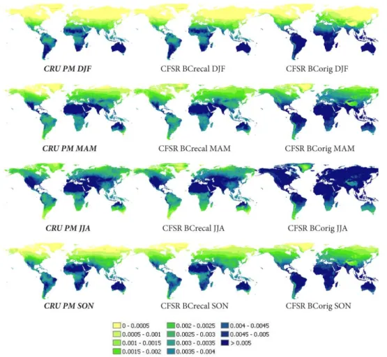
cycle for radiation. PET calculated with the BC equation (CFSRBC) is too high for almost the entire world (Fig. 3c). Overestimations are especially large in Central Africa and Central South-America. The PT equation (CFSRPT) highly overestimates CRUPM in the Amazon basin, Central Africa and Indonesia, whereas underestimations similar to those of PM CFSR PET are present in the Sahara and parts of Aus-tralia (Fig. 3d). By increasing the multiplication factor of the HG equation from 0.0023 to 0.0031, the lowest global average RMSD was obtained (Fig. 3e). PET calculated with the re-calibrated BC equation from the CFSR dataset (CFSR-BCrecal) results in highest similarity with CRUPM (Fig. 3f). For illustrational purpose, global maps of absolute PET val-ues are shown for the different methods in the Supplement (Fig. S1).
3.2.2 Comparison of global seasonal PET
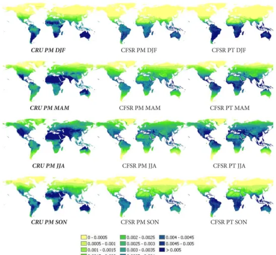
Long-term average seasonal PET maps are given in Fig. 4a, b and c. Figure 4a illustrates that CFSR PM PET is over-all lower than CRU PM PET (Fig. 4a). Notable differences occur over Australia during the SON and MAM season and
over the Sahara throughout the year. Similar deviations over the Sahara can be found for CFSR PT PET, they can be as-signed to the radiation fields used to derive CRU PM, as dis-cussed in Sect. 3.2.1. Yet, also in comparison with the HG and BC methods (Fig. 4b and c), PET over the Sahara is low for the PM and PT equations. CRU PM is overestimated by PT PET over the Southern Hemisphere during the DJF sea-son and over the Amazon throughout the year (Fig. 4a).
Fig. 4a.Global maps with seasonal average daily potential evaporation (m day−1). CRU derived with the Penman-Monteith equation (left; = reference for validation), CFSR derived with the Penman-Monteith equation (middle; PM) and CFSR derived with the Priestley-Taylor equation (right; PT). From top to bottom the DJF, MAM, JJA and SON seasons.
PET values are given for the Mackenzie, Amazon, Rhine and Zambezi river basins in Fig. 5). This may be a result of the use of the equation on a daily instead of monthly time-step, for which the equation was originally designed.
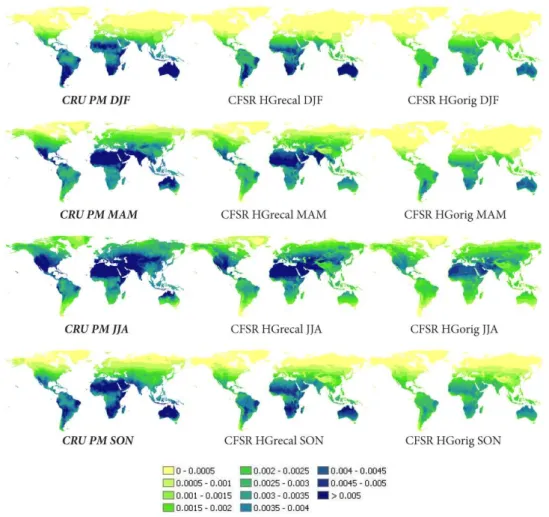
Although the spatial pattern of PET calculated with the HGorig equation highly resembles CRU PET, PET values are globally too low for this method (Fig. 4c). The globally uni-form re-calibration of the HG method notably reduces the differences from CRU PM.
In summary, the HGrecal and BCrecal method show the highest agreement with CRU PET. This result is confirmed by the RMSD statistics calculated from monthly time se-ries. Lowest RMSD values are calculated for the BCrecal and HGrecal equations (Fig. 6e and f). Although the PT and PM method also perform satisfactorily well for some regions, they highly underestimate PET over the Sahara and Australia during winter.
3.3 Impact of different PET equations on actual evapotranspiration and runoff
3.3.1 Long-term average annual evapotranspiration
and runoff
Fig. 4b.Global maps with seasonal average daily potential evaporation (m day−1). CRU derived with the Penman-Monteith equation (left; = reference for validation), CFSR derived with the re-calibrated Blaney-Criddle equation (middle; BCrecal) and CFSR derived with the original Blaney-Criddle equation (right; BCorig). From top to bottom the DJF, MAM, JJA and SON seasons.
maps of seasonal AET values are given in the Supplement (Fig. S2).
Figures 7a, b and 8 show that differences in spatial runoff patterns are almost as small as the differences in AET pat-terns. This is a result of the fact that the runoff flux is in-fluenced by both AET and PR. Runoff is low for the PT and BCorig method (Fig. 7b, panel PT runoff and BCorig runoff). Although increasing the multiplication factor of the original HG equation to 0.0031 resulted in higher PET values, the dif-ference in runoff derived from the two HG time series is still small (Fig. 7a, panel HGrecal runoff and 7b, panel HGorig runoff). Global seasonal runoff maps are provided for the different PET equations in the Supplement (Fig. S3).
3.3.2 Variation between methods
In Fig. 8 the significance of differences (calculated with the Welch’s t-test for a significance level of 95 %) between an-nual average PET, AET and local runoff derived from CFSR data (with any of the PET equations) and annual average
Fig. 4c.Global maps with seasonal average daily potential evaporation (m day−1). CRU derived with the Penman-Monteith equation (left; = reference for validation), CFSR derived with the re-calibrated Hargreaves equation (middle; HGrecal) and CFSR derived with the original Blaney-Criddle equation (right; HGorig). From top to bottom the DJF, MAM, JJA and SON seasons.
Himalayas. Yet, CV values for runoff are low in these re-gions due to the relatively low air temperature, small absolute PET amounts and the large influence of PR. High CV values for PET are also present in the Sahara and central Australia. However, soil moisture is limited in these dry regions and AET amounts are comparably low for the different methods resulting in low CV values.
3.4 Impact of different PET equations on river discharge
3.4.1 Variation between PET methods
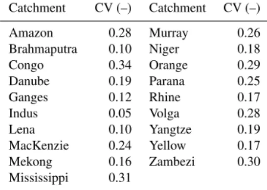
While being illustrative, the differences in runoff obtained from the six methods are hard to distinguish from the global runoff maps (Fig. S3 in the Supplement). Therefore the vari-ation between methods is quantified with basin specific dis-charge CV values, calculated from the disdis-charges using the different CFSR PET time series are listed in Table 3 for 19 large rivers at measurement stations close to the catchment
outlets. The influence of PET methods often decreases while moving within the hydrological model chain from PET to AET to discharge, as water availability becomes limited (V¨or¨osmarty et al., 1998). Basin discharge CV values are found to be lower than CV values for local runoff, due to accumulation of processes along the river network (Sperna Weiland et al., 2012a). CV values of river discharge (Q) range between 0.05 and 0.34 and are on average 0.20.
PM PT BCorig BCrecal HGorig HGrecal
Number of days
Fig. 5.CDFs of daily potential evaporation (m day−1)for a selection of catchments; MacKenzie, Amazon, Rhine and Zambezi.
a) PM AET d) PM runoff
b) HGrecal AET e) HGrecal runoff
c) BCrecal AET f) BCrecal runoff
Fig. 7a. Global maps with on the left annual average daily actual evapotranspiration (m day−1)and on the right annual average daily runoff (m day−1). From top to bottom, Penman-Monteith (PM), Hargreaves with increased multiplication factor (HGrecal) and re-calibrated Blaney-Criddle (BCrecal).
Table 3.Catchment specific coefficients of variation (CV) derived from long-term annual average modeled discharge for measurement stations closest to the catchment outlets, obtained with PET time se-ries calculated with the six different potential evaporation equations.
Catchment CV (–) Catchment CV (–)
Amazon 0.28 Murray 0.26
Brahmaputra 0.10 Niger 0.18
Congo 0.34 Orange 0.29
Danube 0.19 Parana 0.25
Ganges 0.12 Rhine 0.17
Indus 0.05 Volga 0.28
Lena 0.10 Yangtze 0.19
MacKenzie 0.24 Yellow 0.17
Mekong 0.16 Zambezi 0.30
Mississippi 0.31
climate. Contrary to the results of Oudin et al. (2005) this illustrates that for those basins with high CV values, which are unavoidable part of global scale studies, the selection of a PET equation can influence modeled discharge. Only in
regions where both the CV of runoff generated by the differ-ent PET is high and the absolute runoff amounts are of note-worthy value, the selected PET method is likely to have a large impact on modeled runoff and discharge amounts. See for example the Eastern US, parts of Europe, Russia and the Amazon and Congo basin. The decreasing variability be-tween PET methods throughout the modeling chain mainly occurs in arid regions where AET is limited by soil moisture conditions (e.g. the Sahara, Central Australia and the South-Western US) or in the dry seasons.
3.4.2 Deviations from observed GRDC discharge
a) PT AET d) PT runoff
b) HGorig AET e) HGorig runoff
c) BCorig AET f) BCorig runoff
Fig. 7b.Global maps with on the left annual average daily actual evapotranspiration (m day−1)and on the right annual average daily runoff (m day−1). From top to bottom, Priestley-Taylor (PT), the original Hargreaves equation (HGorig) and the original Blaney-Criddle equation (BCorig).
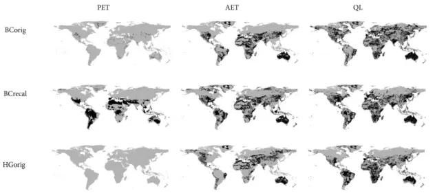
Fig. 8b.Maps showing areas where CFSR derived PET, AET and local runoff (QL) significantly deviates according to the Welch’s t-test for a significance level of 95 % from CRU derived values (in grey) and areas where annual average values do not significantly deviate (in black) for the HGrecal, PM and PT equations.
PET
AET
QL
QC
Fig. 9. Cell specific values of the coefficient of variation (CV; –) calculated from the six different potential evaporation methods for potential evaporation (PET), actual evapotranspiration (AET), local runoff (QL) and discharge (QC).
This is likely a result of this discharge comparison being flawed by measurement errors in amongst others observed discharge (McMillan et al., 2010; Vrugt et al., 2005), bi-ases in PR (Fekete et al., 2004; Biemans et al., 2009) and hydrological model structural errors (Beven, 1996; Vrugt et al., 2005). The most extreme model results are compensat-ing for these biases. This can clearly be seen for the BCorig method, which overall results in the lowest discharge val-ues and therefore performs best for the arid basins (e.g. the Murray, Orange, Zambezi and Niger) where the hydrologi-cal model generally overestimates observed discharge (Van Beek, 2008). Because of these biases no clear conclusions can be drawn from the comparison.
4 Conclusions
In this study six different methods, to globally derive daily PET time series from CFSR reanalysis data, have been eval-uated on (1) their resemblance with monthly PET time series calculated from the CRU datasets with the Penman-Monteith equation and (2) their impact on modeled AET, runoff and river discharge and consequently usability for hydrological impact studies. From the analysis above the following con-clusions can be drawn:
Fig. 10.Long-term average annual basin discharge (km3yr−1) for 19 large river basins derived with PCRGLOB-WB forced with the CFSR dataset where potential evaporation was calculated using one of the six different PET methods (group of bars on the right for each river). As a reference long-term average corrected observed GRDC basin discharge has been included (black; periods do not completely overlap due to limited data availability).
throughout the hydrological modeling chain (i.e. from PET, AET, runoff to discharge) for these basins. Nevertheless the selected PET method is likely to have a high impact on runoff and discharge amounts for some specific regions (e.g. Ama-zon, Congo and Mississippi regions). This stresses the ne-cessity to select the most accurate and spatially stable PET method.
Overall, the re-calibrated forms of the Blaney-Criddle and Hargreaves equations applied to CFSR data seemed to be best suited to derive daily PET times series. Within this study the Penman-Monteith equation, applied to CFSR data, does not outperform the other methods. It should be noted that this may as well be a result of inaccuracies in individual at-mospheric variables in the CRU and CFSR datasets. The sensitivity analysis in Sect. 3.1 illustrated that especially the difference in wind and radiation used for the calculation of CFSR and CRU Penman-Monteith potential evaporation in-troduces large differences. Due to its high input data require-ments and its sensitivity to input data accuracy, the Penman-Monteith method is likely to be less suited for climate change studies.
However, we pose two critical remarks against the use of the re-calibrated form of Blaney-Criddle method. First, dis-charge derived with the re-calibrated Blaney-Criddle method is too low compared to the other methods for most basins. Second, the high spatial variability in the Blaney-Criddle re-calibrated coefficient values (Fig. 1) suggests that are sensi-tive towards future changing climate conditions.
We therefore recommend the re-calibrated form of the Hargreaves equation for the derivation of consistent daily PET time series from CFSR reanalysis data for global hy-drological studies. Due to its small and spatial uniform bias, the modified Hargreaves method performs satisfactorily in multiple climate zones. In its re-calibrated form the multi-plication factor was increased from 0.0023 to 0.0031, which significantly decreased the deviations from CRU PET. Yet, to fully confirm that the re-calibrated Hargreaves method is also stable under changing climate conditions, further inves-tigation with future climate datasets is needed.
The results of this study can be of great value for future climate impact assessments. The created PET time series are currently being used to downscale daily PET times-series de-rived from raw GCM data. These downscaled projections are then used to force the global hydrological model PCR-GLOBWB which will result in new consistent hydrological projections at the global scale. The global gridded PET-time-series can be downloaded from http://opendap.deltares. nl/thredds/dodsC/opendap/deltares/FEWS-IPCC.
Supplementary material related to this article is available online at:
http://www.hydrol-earth-syst-sci.net/16/983/2012/ hess-16-983-2012-supplement.pdf.
Acknowledgements. The global discharge time series have been obtained from the Global Runoff Data Centre. The CFSR reanal-ysis products used in this study are obtained from the Research Data Archive (RDA) which is maintained by the Computational and Information Systems Laboratory (CISL) at the National Center for Atmospheric Research (NCAR). NCAR is sponsored by the National Science Foundation (NSF). The original data are available from the RDA (http://dss.ucar.edu) in dataset number ds093.0. H. H. D¨urr was partly funded by the EU FP6 program “Carbo-North” (contract no. 036993), C. Tisseuil was funded by the Biofresh (contract no. 226874) 7th Framework European project and F. C. Sperna Weiland was funded by the Dutch Research Institute Deltares.
References
Allen, R. G.: Evaluation of a temperature difference method for computing grass reference evapotranspiration, Report submitted to the Water Resources Development and Man Service, Land and Water Development Division, FAO, Rome, 49 pp., 1993. Allen, R. G., Pereira, L. S., Raes, D., and Smith, M.: Crop
evapo-transpiration: FAO Irrigation and drainage paper 56, FAO, Rome, Italy, 1998.
Arnell, N. W.: The effect of cliamte change on hydrological regimes in Europe: a continental perspective, Global Environ. Chang., 9, 5–23, 1999.
Arnell, N. W.: Uncertainty in the relationship between climate forc-ing and hydrological response in UK catchments, Hydrol. Earth Syst. Sci., 15, 897–912, doi:10.5194/hess-15-897-2011, 2011. Beven, K.: A discussion of distributed hydrological modelling, in:
Distributed Hydrological Modelling, Abbott MB, edited by: Ref-sgaard, J. C., Kluwer Academic; 255–278, 1996.
Biemans, H., Hutjes, R. W. A., Kabat, P., Strengers, B., Gerten, D., and Rost, S.: Effects of precipitation uncertainty on discharge calculations for main river basins, J. Hydrometeorol., 10, 1011– 1025, doi:10.1175/2008JHM1067.1, 2009.
Blaney, H. F. and Criddle, W. P.: Determining water requirements in irrigated areas from climatological and irrigation data, USDA (SCS) TP-96, 48 pp., 1950.
Boorman, H.: Sensitivity analysis of 18 different potential evapotranspiration models to observed climatic change at German climate stations, Climatic Change, 104, 729–753, doi:10.1007/s10584-010-9869-7, 2010.
D¨oll, P. and Lehner, B.: Validating of a new global 30-minute drainage direction map, J. Hydrol., 258, 214–231, 2002. Droogers, P. and Allen, R. G.: Estimating reference
evapotranspi-ration under inaccurate data conditions, Irrig. Drain. Syst., 16, 33–45, 2002.
Ekstr¨om, M., Jones, P. D., Fowler, H. J., Lenderink, G., Buishand, T. A., and Conway, D.: Regional climate model data used within the SWURVE project – 1: projected changes in seasonal patterns and estimation of PET, Hydrol. Earth Syst. Sci., 11, 1069–1083, doi:10.5194/hess-11-1069-2007, 2007.
Elshamy, M. E., Seierstad, I. A., and Sorteberg, A.: Impacts of cli-mate change on Blue Nile flows using bias-corrected GCM sce-narios, Hydrol. Earth Syst. Sci., 13, 551–565, doi:10.5194/hess-13-551-2009, 2009.
Fekete, B. M., V¨or¨osmarty, C. J., Roads, J. O., and Willmott, C. J.: Uncertainties in precipitation and their impacts on runoff es-timates, J. Climate, 17, 294–304, 2004.
Gavilan, P., Lorite, I. J., Tornero, S., and Berengena, J.: Regional calibration of Hargreaves equation for estimating reference ET in a semiarid environment, Agr. Water Manage., 81, 257–281, doi:10.1016/j.agwat.2005.05.001, 2006.
GRDC: Major River Basins of the World/Global Runoff Data Cen-tre, D-56002, Koblenz, Federal Institute of Hydrology (BfG), 2007.
Hagemann, S. and D¨umenil Gates, L.: Improving a subgrid runoff parameterization scheme for climate models by the use of high resolution data derived from satellite observations, Clim. Dy-nam., 21, 349–359, 2003
Hargreaves, G. H. and Samani, Z. A.: Reference crop evapotranspi-ration from temperature, Appl. Eng. Agric., 1, 96–99, 1985. Hargreaves, G. H., Asce, F., and Allen, R. G.: History and
evalu-ation of Hargreaves evapotranspirevalu-ation equevalu-ation, J. Irrig. Drain. E.-ASCE, 129, 53–63, 2003.
Higgins, R. W., Kousky, V. E., Silva, V. B. S., Becker, E., and Xie, P.: Intercomparison of Daily Precipitation Statistics over the United States in Observations and in NCEP Reanalysis Products, J. Climate, 23, 4637–4650, doi:10.1175/2010JCLI3638.1, 2010. IPCC: Climate change 2007: Synthesis report – summary for policy
makers, 22 pp., 2007.
Jensen, M. E.: Discussion of “irrigation water requirements of lawns”, J. Irr. Drain. Div.-ASCE, 92, 95–100, 1966.
Kalnay, E., Kanamitsu, M., Kistler, R., Collins, W., Deaven, D., Gandin, L., Iredell, M., Saha, S., White, G., Woollen, J., Zhu, Y., Leetmaa, A., Reynolds, R., Chelliah, M., Ebisuzaki, W., Higgins, W., Janowiak, J., Mo, K. C., Ropelewski, C., Wang, J., Jenne, R., and Joseph, D.: The NCEP/NCAR 40-year reanalysis project, B. Am. Meteorol. Soc., 77, 437–470, 1996.
Kay, A. L. and Davies, V. A.: Calculating potential evapora-tion from climate model data: A source of uncertainty for hy-drological climate change impacts, J. Hydrol., 358, 221–239, doi:10.1016/j.jhydrol.2008.06.005, 2008.
Kingston, D. G., Todd, M. C., Taylor, R. G., and Thompson, J. R.: Uncertainty in the estimation of potential evapotranspira-tion under climate change, Geophys. Res. Lett., 36, L20403, doi:10.1029/2009GL040267, 2009.
Loveland, T. R., Reed, B. C., Brown, J. F., Ohlen, D. O., Zhu, J., Yang, L., and Merchant, J. W.: Development of a Global Land Cover Characteristics Database and IGBP DISCover from 1-km AVHRR Data, Int. J. Remote Sens., 21, 1303–1330, 2000. Lu, J., Sun, G., McNulty, S. G., and Amatya, D. M.: A comparison
of six potential evapotranspiration methods for regional use in the southeastern united states, J. Am. Water Resour. As., 41, 621– 633, 2005.
Mahanama, S. P. P. and Koster, R. D.: AGCM biases in evaporation regime: Impacts on soil moisture memory and land-atmosphere feedback, J. Hydrometeorol., 6, 656–669, doi:10.1175/JHM446.1, 2005.
Maurer, E. P., Hidalgo, H. G., Das, T., Dettinger, M. D., and Cayan, D. R.: The utility of daily large-scale climate data in the assess-ment of climate change impacts on daily streamflow in Califor-nia, Hydrol. Earth Syst. Sci., 14, 1125–1138, doi:10.5194/hess-14-1125-2010, 2010.
McMillan, H., Freer, J., Pappenberger, F., Krueger, T., and Clark, M.: Impacts of uncertain river flow data on rainfall-runoff model calibration and discharge predictions, Hydrol. Process., 24, 1270–1284, 2010.
Michelangeli, P.-A., Vrac, M., and Loukos, H.: Probabilis-tic downscaling approaches: application to wind cumula-tive distribution functions, Geophys. Res. Lett., 36, L11708, doi:10.1029/2009GL038401, 2009.
Mitchell, T. D. and Jones, P. D.: An improved method of con-structing a database of monthly climate observations and as-sociated high-resolution grids, Int. J. Climatol., 25, 693–712, doi:10.1002/joc.1181, 2005.
Monteith, J. L.: Evaporation and environment, Sym. Soc. Exp. Biol., 19, 205–234, 1965.
New, M., Hulme, M., and Jones, P.: Representing Twentieth-Century Space-Time Climate Variability. Part II: Development of 1901–96 Monthly Grids of Terrestrial Surface Climate, J. Cli-mate, 13, 2217–2238, 2000.
Oudin, L., Hervieu, F., Michel, C., Perrin, C., Andr´eassian, V., Anctil, F., and Loumagne, C.: Which potential evapotran-spiration input for a lumped rainfall-runoff model? Part 2 – Towards a simple and efficient potential evapotranspiration model for rainfall-runoff modelling, J. Hydrol., 303, 290–306, doi:10.1016/j.jhydrol.2004.08.026, 2005.
PCMDI: Program for Climate Model Diagnosis and Intercompar-ison data portal, available at: https://esg.llnl.gov:8443/index.jsp (last access: 20 March 2012), 2010.
Piani, C., Weedon, G. P., Best, M., Gomes, S. M., Viterbo, P., Hagemann, S., and Haerter, J. O.: Statistical bias correction of global simulated daily precipitation and temperature for the application of hydrological models, J. Hydrol., 395, 199–215, doi:10.1016/j.jhydrol.2010.10.024, 2010.
Priestley, C. H. B. and Taylor, R. J.: On the assessment of surface heat flux and evaporation using large-scale parameters, Mon. Weather Rev., 100, 81–92, 1972.
Roderick, L. M., Rotstayn, L. D., Farquhar, G. D., and Hobbins, M. T.: On the attribution of changing pan evaporation, Geophys. Res. Lett., 34, L17403, doi:10.1029/2007GL031166, 2007. Saha, S., Nadiga, S., Thiaw, C., Wang, J., Wang, W., Zhang, Q.,
van den Dool, H. M., Pan, H. L., Moorthi, S., Behringer, D., Stokes, D., Pe˜na, M., Lord, S., White, G., Ebisuzaki, W., Peng, P., and Xie, P.: The NCEP Climate Forecast System, J. Climate, 19, 3483–3517, 2006.
Saha, S., Moorthi, S., Pan, H.-L., Wu, X., Wang, J., Nadiga, S., Tripp, P., Kistler, R., Woollen, J., Behringer, D., Liu, H., Stokes, D., Grumbine, R., Gayno, G., Wang, J., Hou, Y.-T., Chuang, H.-Y., Juang, H.-M. H., Sela, J., Iredell, M., Treadon, R., Kleist, D., van Delst, P., Keyser, D., Derber, J., Ek, M., Meng, J., Wei, H., Yang, R., Lord, S., van den Dool, H., Kumar, A., Wang, W., Long, C., Chelliah, M., Xue, Y., Huang, B., Schemm, J.-K., Ebisuzaki, W., Lin, R., Xie, P., Chen, M., Zhou, S., Higgins, W., Zou, C.-Z., Liu, Q., Chen, Y., Han, Y., Cucurull, L., Reynolds, R. W., Rutledge, G., and Goldberg, M.: The NCEP Climate Fore-cast System Reanalysis, B. Am. Meteorol. Soc., 91, 1015–1057, 2010.
Sperna Weiland, F. C., van Beek, L. P. H., Kwadijk, J. C. J., and Bierkens, M. F. P.: The ability of a GCM-forced hydro-logical model to reproduce global discharge variability, Hy-drol. Earth Syst. Sci., 14, 1595–1621, doi:10.5194/hess-14-1595-2010, 2010.
Sperna Weiland, F. C., van Beek, L. P. H., Kwadijk, J. C. J., and Bierkens, M. F. P.: On the suitability of GCM runoff fields for river discharge modeling; a case study using model output from HadGEM2 and ECHAM5, J. Hydrometeorol., J. Hydrometeo-rol., 13, 140–154, doi:10.1175/JHM-D-10-05011.1, 2012a. Sperna Weiland, F. C., van Beek, L. P. H., Kwadijk, J. C. J., and
Bierkens, M. F. P.: Global patterns of change in runoff regimes for 2100, Hydrol. Earth Syst. Sci. Discuss., accepted, 2012b. Van Beek, L. P. H.: Forcing PCR-GLOBWB with CRU
data, Utrecht University, available at: http://vanbeek.geo.uu.nl/ suppinfo/vanbeek2008.pdf (last access: 24 March 2012), 2008. Van Beek, L. P. H., Wada, Y., and Bierkens, M. F. P.: Global
monthly water stress: I. Water balance and water availability, Water Resour. Res., online first: doi:10.1029/2010WR009791, 2011.
V¨or¨osmarty, C. J., Federer, C. A., and Schloss, A. L.: Poten-tial evaporation functions compared on U.S. watersheds: Pos-sible implications for global-scale water balance and terrestrial ecosystem modeling, J. Hydrol., 207, 147–169, 1998.
Vrugt, J. A., Diks, C. G. H., Gupta, H. V., Bouten, W., and Verstraten, J. M.: Improved treatment of uncertainty in hydro-logic modeling: Combining the strengths of global optimiza-tion and data assimilaoptimiza-tion, Water Resour. Res., 41, W01017, doi:10.1029/2004WR003059, 2005.
Wada, Y., Van Beek, L. P. H., Van Kempen, C. M., Reckman, J. W. T. M., Vasak, S., and Bierkens, M. F. P.: Global deple-tion of groundwater resources, Geophys. Res. Lett., 37, L20402, doi:10.1029/2010GL044571, 2010.
Weiß, M. and Menzel, L.: A global comparison of four potential evapotranspiration equations and their relevance to stream flow modelling in semi-arid environments, Adv. Geosci., 18, 15–23, 2008,
http://www.adv-geosci.net/18/15/2008/.
Welch, B. L.: The generalization of “Student’s” problem when sev-eral different population variances are involved, Biometrika, 34, 28–35, doi:10.1093/biomet/34.1-2.28, 1947.