A framework for evaluating regional hydrologic sensitivity to climate change using archetypal watershed modeling

(1)

HESSD

9, 13729–13771, 2012

A framework for evaluating regional hydrologic sensitivity

S. R. Lopez et al.

Title Page

Abstract Introduction

Conclusions References

Tables Figures

◭ ◮

Back Close

Full Screen / Esc

Printer-friendly Version

Interactive Discussion

Discussion

P

a

per

|

Dis

cussion

P

a

per

|

Discussion

P

a

per

|

Discussio

n

P

a

per

|

Hydrol. Earth Syst. Sci. Discuss., 9, 13729–13771, 2012 www.hydrol-earth-syst-sci-discuss.net/9/13729/2012/ doi:10.5194/hessd-9-13729-2012

Hydrology and Earth System Sciences Discussions

This discussion paper is/has been under review for the journal Hydrology and Earth System Sciences (HESS). Please refer to the corresponding final paper in HESS if available.

A framework for evaluating regional

hydrologic sensitivity to climate change

using archetypal watershed modeling

S. R. Lopez1,*, T. S. Hogue1,*, and E. D. Stein2

1

Department of Civil and Environmental Engineering, University of California, Los Angeles, USA

2

Southern California Coastal Water Research Project, Costa Mesa, CA, USA *

now at: Colorado School of Mines, Golden, CO, USA

Received: 5 October 2012 – Accepted: 20 November 2012 – Published: 14 December 2012

Correspondence to: T. S. Hogue (thogue@mines.edu)

(2)

HESSD

9, 13729–13771, 2012

S. R. Lopez et al.

Title Page

Tables Figures

◭ ◮

Back Close

Full Screen / Esc

Discussion

P

a

per

|

Dis

cussion

P

a

per

|

Discussion

P

a

per

|

Discussio

n

P

a

per

|

Abstract

The current study focuses on the development of a regional framework to evaluate hydrologic and sediment sensitivity due to predicted future climate variability using developed archetypal watersheds. The developed archetypes are quasi-synthetic wa-tersheds that integrate observed regional physiographic features (i.e., geomorphology, 5

land cover patterns, etc.) with synthetic derivation of basin and reach networks. Each of the three regional archetypes (urban, vegetated and mixed land covers) simulates sat-isfactory hydrologic and sediment behavior compared to historical observations (flow and sediment) prior to the climate sensitivity analysis. Climate scenarios considered increasing temperature estimated from the IPCC and precipitation variability based on 10

historical observations and expectations. Archetypal watersheds are modeled using the Environmental Protection Agency’s Hydrologic Simulation Program–Fortran model (EPA HSPF) and relative changes to streamflow and sediment flux are evaluated. Re-sults indicate that the variability and extent of vegetation play a key role in watershed sensitivity to predicted climate change. Temperature increase alone causes a decrease 15

in annual flow and an increase in sediment flux within the vegetated archetypal wa-tershed only, and these e_ffects are partially mitigated by the presence of impervious surfaces within the urban and mixed archetypal watersheds. Depending on extent of precipitation variability, urban and moderately urban systems can expect the largest al-teration to flow regimes where high flow events are expected to become more frequent. 20

As a result, enhanced wash-off of suspended-sediments from available pervious sur-faces is expected.

1 Introduction

Numerous reports by the Intergovernmental Panel on Climate Change (1992, 1995,

2001 and 2007) predict global mean temperatures may increase from 1.4 to 5.8◦C

25

(3)

HESSD

9, 13729–13771, 2012

S. R. Lopez et al.

Title Page

Tables Figures

◭ ◮

Back Close

Full Screen / Esc

Discussion

P

a

per

|

Dis

cussion

P

a

per

|

Discussion

P

a

per

|

Discussio

n

P

a

per

|

snow accumulation and melt, river runoff, soil moisture storage and plant water avail-ability (McCabe and Wolock, 2008; Costa and Soares, 2009; Githui et al., 2009; Hi-dalgo et al., 2009; Kunkel et al., 2009; Clark, 2010; Wang et al., 2010). Climate-induced anomalies have significant consequences for water-stressed regions (Mote et al., 2005; CCCC, 2006; Arag ˜ao et al., 2007; Westerling and Bryant, 2008). In the 5

southwestern United States, potential and observed impacts of climate change have

been summarized in numerous research efforts (Knowles and Cayan 2002; Kiparsky

and Gleick, 2003; Miller et al., 2003; Hayhoe et al., 2004; Kim, 2005; Mote et al., 2005; CAT, 2009). Several studies have focused on addressing climate change and impacts to water resources in snow-prevalent regions of Northern California (Gleick 10

and Chalecki, 1999; Christensen et al., 2004; Hayhoe et al., 2004; Mote et al., 2005; McCabe and Wolock, 2008), but few studies have evaluated climate impacts in the southern region of the state. Southern California contains rapidly growing metropoli-tan areas with a projected population growth of 40 % by 2050 (California Department of Finance 2007). Potential losses of surface or groundwater resources in the region 15

will ultimately strain a water system heavily dependent on imported water and hamper efforts to make the region more locally sustainable.

The traditional approach for predicting future large-scale climate response is through the use of General Circulation Models (GCMs) (10–100 s km2); however, these coarse resolution models are incapable of resolving regional to local-scale processes that are 20

essential in determining finer-scale effects relevant to societal concerns and local deci-sion making (e.g., water quality and availability, energy use, air quality, storm severity, etc.). Efforts to use GCM output at the local or watershed scale have led to the de-velopment of statistical (using historical and GCM output) and dynamic (using GCM output and coupled regional models) downscaling methods. Although both these ap-25

(4)

HESSD

9, 13729–13771, 2012

S. R. Lopez et al.

Title Page

Tables Figures

◭ ◮

Back Close

Full Screen / Esc

Discussion

P

a

per

|

Dis

cussion

P

a

per

|

Discussion

P

a

per

|

Discussio

n

P

a

per

|

A range of simple approaches have been developed to evaluate potential changes in runo_ff and sedimentation, including performing sensitivity analyses on watershed systems and varying parameters such as land cover, precipitation, temperature and evapotranspiration (DeWalle and Swistock, 2000; Pruski and Nearing, 2002; Singer and Dunne, 2004; Nearing et al., 2005; Soboll, 2011). This approach does not require 5

advanced statistical methodologies or extensive computing. Random variability (wet day frequency and precipitation amount) is generally added to the precipitation time-series, whereas an increase or decrease in temperature range is added to historical temperature. By altering historical time-series, the user is able to develop relatively robust scenarios to evaluate watershed hydrologic and sediment response due to ex-10

pected variability in climate.

The goal of the current work is to develop a user-friendly and efficient framework to quantify the sensitivity of hydrologic and sediment behavior to climate variability across a large region in southern California. This is accomplished by developing regional quasi-synthetic watershed archetypes based on observed regional physiographic fea-15

tures and investigating the effects of varying climate on runoff using an operational environmental and water resource model, the Hydrologic Simulation Program–Fortran (HSPF), that has been applied across southern California (Ackerman et al., 2005; Ban-durraga, 2011; He and Hogue, 2011; Hevesi et al., 2011). The regional archetypes are quasi-synthetic watersheds that use observed regional physiographic features (i.e., ge-20

omorphology, land cover patterns, etc.) and synthetic derivation of basin and reach net-works. Each regional archetype simulates representative short-term (daily) and long-term (annual) hydrologic and sediment behavior prior to the climate sensitivity analy-sis. The current study deviates from traditional methods because it obtains information beyond a single watershed-scale analysis and also avoids use of a macro-scale hydro-25

(5)

HESSD

9, 13729–13771, 2012

S. R. Lopez et al.

Title Page

Tables Figures

◭ ◮

Back Close

Full Screen / Esc

Discussion

P

a

per

|

Dis

cussion

P

a

per

|

Discussion

P

a

per

|

Discussio

n

P

a

per

|

2 Methods

2.1 Study region and data

The selected study area is the southern California coast, from south of Santa Barbara to the US-Mexico Border. The region is characterized by a mediterranean-type climate with precipitation ranging from 6 to 40 inches and mean annual temperature ranging 5

from 61 to 65◦F (16 to 18◦C) (Levien et al., 2002). Lower elevation vegetation (below 6000 ft.) is predominantly chaparral and scrubs, while forested communities are found at elevations above 6000 feet (Levien et al., 2002). Counties within southern California also have varying levels of urban and built-up land ranging from 32 % to 91 % (California Department of Conservation – Division of Land Resource Protection 2011).

10

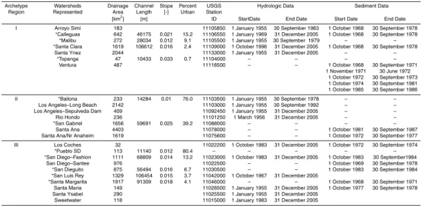
Observed physiographic information including land cover, soil type, drainage area, channel length and channel slope were gathered for selected coastal southern Cal-ifornia watersheds (Table 1). Land cover distribution was obtained using the NOAA Coastal Change Assessment Program (CCAP) data, which is based on 30 m LAND-SAT imagery (NOAA-CSC 2003). The data was originally classified into 39 land types; 15

however, extensive land cover classifications were unnecessary for the purpose of this project. Similar classifications (i.e., Chaparral and Chaparral Park; Sage and Sage Park; etc.) were combined resulting in 23 land cover types.

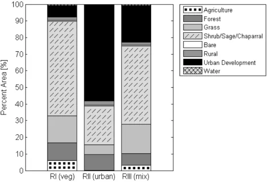
The observed distribution of physiographic properties as well as regional climate patterns (Nezlin and Stein, 2005) were used to subset the study area into three regions 20

(for three proposed archetypes): Region I includes Ventura County watersheds with minimal urbanization vegetated with Scrub/Shrub, Sage and Chaparral (typical plant-type in southern California), Region II represents the Los Angeles region with relatively dense urbanization and little natural land cover, and Region III spans the San Diego area which has an observed mix of vegetated and urban land types (Fig. 1). The mean 25

(6)

HESSD

9, 13729–13771, 2012

S. R. Lopez et al.

Title Page

Tables Figures

◭ ◮

Back Close

Full Screen / Esc

Discussion

P

a

per

|

Dis

cussion

P

a

per

|

Discussion

P

a

per

|

Discussio

n

P

a

per

|

39 and 75 %, respectively. Distinguished by climate and land cover differences, the three systems along the coastline are defined as Vegetated (Region I), Urban (Region II), and Mixed (Region III).

A time-series of representative climatology were gathered for each defined region. Based on prior work in southern Calfornia (Nezlin and Stein, 2005), we advocate that 5

selecting a gauge within each distinct region provides reasonable estimation of cli-matology for each defined region. Hourly meteorological observations from proximal airport stations within each region were used: Santa Maria (CA007946), Los Ange-les International (CA005114) and San Diego (CA007740) (EPA, 2009). Each time series contains precipitation, temperature and related meteorological variables from 10

1 January 1950 to 31 December 2005 (55 yr). Within this time frame there were sub-stantial inter-annual variability with 16 El Ni ˜no events and 18 La Ni ˜na events (NOAA-NWS 2010). Historical flow and sediment concentration data (USGS 2009) were also gathered from regional watersheds (Table 1) to utilize for classification of the regional systems as well as for model evaluation.

15

2.2 Development of archetypal watersheds

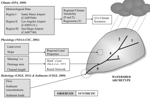
Each archetypal watershed was developed to serve as a representative model for that region and provide reasonable simulations of hydrologic and suspended sediment loads within the framework. Observed data sets (climate, physiology, hydrology and sediment) were used to develop the archetypes and establish the physical construct 20

(Fig. 2). Mean regional land cover and slope were directly integrated into developing the archetype; however, the large variability in channel length, drainage size and reach network led to the exploration of more synthetic approaches for these parameters. The drainage area (259 km2; 100 mi2) and number of reaches (5) were held constant for each archetype in order to constrain variability in system response due to size and 25

(7)

HESSD

9, 13729–13771, 2012

S. R. Lopez et al.

Title Page

Tables Figures

◭ ◮

Back Close

Full Screen / Esc

Discussion

P

a

per

|

Dis

cussion

P

a

per

|

Discussion

P

a

per

|

Discussio

n

P

a

per

|

[A; square miles] (Hack et al., 1957) and defined as:

L₌1.4A0.6 (1)

Using the archetypal watershed area of 259 km2and the corresponding total channel length of 35.8 km, the remaining reach properties were designed based on evaluation and general knowledge of typical drainage systems in southern California. Reaches 1 5

2, 4 and 5 were set at one-third the total channel length (11.9 km) and reach 3 was set at one-sixth the total channel length (6 km). Reaches 2, 4 and 5 are considered the main channel and Reaches 1 and 3 are contributing to the stream network (Fig. 2). Contributing drainage area for each reach is set at one-sixth the total area with the exception of reach 5, the outlet stream, which is assumed to be one-third the entire 10

basin. The change in elevation for each reach is a function of the reach length and the overall slope of the channel based on slope measurements within each respec-tive region (Table 1). Manning’s roughness coefficient for overland flow (NSUR) for pervious and impervious surfaces was 0.2 and 0.1, respectively, for all watersheds. These surface coefficients have also been used in the HSPF model for southern Cal-15

ifornia (He and Hogue, 2011; Ackerman, 2005). The Manning’s nchannel coefficient for each region was determined based on the predetermined land cover classifica-tion. Region I’s channels are assumed primarily natural (n₌0.04), Region II channels are cement (n₌0.01) and Region III Manning’s n is a mixture of cement and natu-ral reaches (n₌0.025). Model sensitivity for Manning’snwas primarily noted with the 20

channel coefficient.

2.2.1 Archetypal model assumptions

The vegetated archetypal watershed (Region I) represents areas with a higher per-centage of pervious land cover, which generally promotes surface infiltration and re-duces streamflow. Sediment yield is expected to be higher in the vegetated archetypal 25

(8)

HESSD

9, 13729–13771, 2012

S. R. Lopez et al.

Title Page

Tables Figures

◭ ◮

Back Close

Full Screen / Esc

Discussion

P

a

per

|

Dis

cussion

P

a

per

|

Discussion

P

a

per

|

Discussio

n

P

a

per

|

(Trimble, 1997). The urban archetypal watershed (Region II) should exhibit more in-tense, high flow output and low sediment flux, characteristic of urban watersheds with cement-lined channel systems. Streambed erosion from the remaining natural chan-nels can be accelerated in urban systems if the frequency and magnitude of peak discharge increases due to runo_ff from impervious surfaces (Trimble, 1997). Region 5

III’s archetypal watershed is considered an area that is increasing in urbanization and may experience sediment and flow patterns that reside between the vegetated and fully urbanized systems; lower flow patterns than the urban archetype and lower sediment loads than the vegetated system. No dams or upstream obstructions were integrated into the archetypal models in this initial work. Changes to land cover are not explored 10

within this study because the archetypal systems are designed to represent the current range of urbanization patterns in southern California.

2.3 Model description

The Hydrologic Simulation Program-Fortran (HSPF) simulates watershed hydrology and movement of contaminants including fate and transport of sediment, pesticides, 15

nutrients and other water quality parameters in stream systems (Bicknell et al., 2000). The HSPF model was chosen because it has been used in previous studies conducted in southern California counties: Ventura (Bandurraga, 2011), San Bernardino (Hevesi et al., 2011) and Los Angeles (Ackerman et al., 2005; He and Hogue, 2011) and is used by the EPA for watershed investigations.

20

Precipitation, temperature and estimations of potential evaporation are required in-puts for HSPF. Three modules are needed for simulation of watershed hydrology: PERLND, IMPLND and RCHRES. The PERLND (pervious surfaces) and IMPLND (im-pervious surfaces) modules require land cover classification and several geo-physical characteristics and RCHRES (streams) requires physical dimensions (length, slope, 25

(9)

HESSD

9, 13729–13771, 2012

S. R. Lopez et al.

Title Page

Tables Figures

◭ ◮

Back Close

Full Screen / Esc

Discussion

P

a

per

|

Dis

cussion

P

a

per

|

Discussion

P

a

per

|

Discussio

n

P

a

per

|

surface runoff/infiltration is governed by Philips equation (Philips, 1957). Runoffthen moves laterally to down-slope segments or to a river reach or reservoir. Other sim-ulated processes include interception, percolation, interflow, and groundwater move-ment. The HSPF applies Manning’s Equation for routing overland flow and kinematic wave for channel routing.

5

Sediment simulation is performed using three modules: SEDMNT (pervious sur-faces), SOLIDS (impervious surfaces) and SEDTRN (stream transport). Sediment from pervious land cover detaches the soil surface and enters the stream result via overland flow (Bicknell, 2000). Solids from impervious surfaces wash-offdue to a precipitation event; the load is primarily driven by the rate of accumulation of solid materials (Bick-10

nell, 2000). Stream sediments are initialized by specifying clay, silt, sand fractions and result from processes such as deposition, scour and transport (Bicknell, 2000). Sum-mation of sediments from all three modules results in the total sediment load.

Modeling was undertaken for all archetypal watersheds using the following data sets: Historical observations (1955–2005) and 21 future climate scenarios (50 yr period) (de-15

scribed in Sect. 2.4). A five-year spin-up period (not used in final analysis) was included in all model simulations. The model was run at an hourly time-step using the meteoro-logical data from the three proximal airport stations for each region.

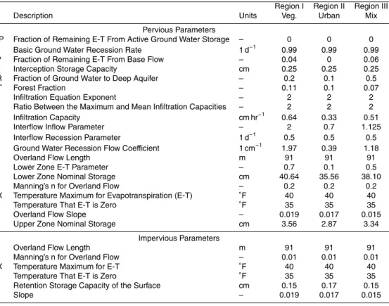
2.3.1 Parameter selection

Hydrologic parameter values were initialized using previous work within southern Cal-20

ifornia (He and Hogue, 2011; Ackerman et al., 2005). PERLND and IMPLND hydrol-ogy parameters were determined first by comparing simulated outputs to observations from watersheds within the three study regions. The list of watersheds and hydrologic data gathered from the United States Geological Survey (USGS 2011) are provided in Table 1. Daily observations were used to assure model behavior was within regional 25

(10)

HESSD

9, 13729–13771, 2012

S. R. Lopez et al.

Title Page

Tables Figures

◭ ◮

Back Close

Full Screen / Esc

Discussion

P

a

per

|

Dis

cussion

P

a

per

|

Discussion

P

a

per

|

Discussio

n

P

a

per

|

Nash-Sutcliffe Efficiency (NSE), Percent Bias (BIAS) and Pearson’s Correlation Co-efficient (R2) Eqs. (2–5):

RMSE=

v u u

t1

n

X

i=1

(Q_sim,t₋Q_obs,t)2 ₍₂₎

% BLAS=

Pn

t=1(Qsim,t−Qobs,t)

Pn

t=1(Qobs,t)

!

×100 (3)

5

NSE₌1− −

Pn

t=1(Qsim,t−Qobs,t) 2

Pn

t=1(Qobs,t−Q¯obs)2

!

(4)

R2₌



 

nPn

t₌1Qsim,tQobs,t−(

P

Q_sim,t)(Pn

t₌1Qobs,t)

q

n(Pn

t₌1Q 2 sim,t)−(

Pn

t₌1Qsim,t)2

q

n(Pn

t₌1Q 2 obs,t)−(

Pn

t₌1Qobs,t)2



 

2

(5)

For each of the above formulations Q_sim, is the simulated flow, Q_obs is the observed 10

flow, ¯Q_obs is the overall mean observed flow,nis the total number of observations, and t is the time-step used for statistical comparison. Annual comparisons were also made using long-term runoffratios from observed and archetypal watersheds.

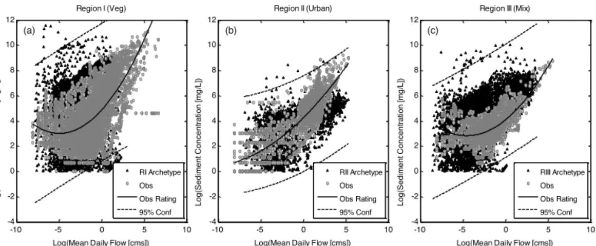
Observed suspended-sediment and flow data (Table 1) were compared to archetypal simulations using log (concentration)-log (discharge) rating curves. Rating curves were 15

(11)

HESSD

9, 13729–13771, 2012

S. R. Lopez et al.

Title Page

Tables Figures

◭ ◮

Back Close

Full Screen / Esc

Discussion

P

a

per

|

Dis

cussion

P

a

per

|

Discussion

P

a

per

|

Discussio

n

P

a

per

|

Rating curves were used to compare long-term sediment simulations instead of per-forming analysis on a storm-by-storm basis. An initial shortcoming in calibrating sedi-ment was availability of long-term observations. In order to be confident in the long-term simulations of mean annual sediment flux (t yr−1), simulations were also compared to observations provided by Inman and Jenkins (1999) for the 1969–1995 data period. 5

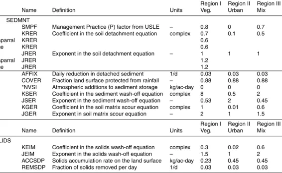
Final parameter values for hydrologic and sediment simulations are summarized in Tables 2 and 3. The vegetated archetypal watershed (Region I) in our study required the separation of the coe_fficient (KRER) and exponent (JRER) of the soil detachment equation, in order to obtain reasonable sediment estimates based on observed results. The change in these parameter values was applied to Chaparral and Sage land covers, 10

the two dominant natural land cover types in Region I.

2.4 Development of climate scenarios

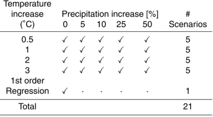
To evaluate each archetypal watershed’s sensitivity to climate variability, historical pre-cipitation and temperature time series were perturbed to serve as input to the HSPF model for each region. Changes to temperature were based on 1st order regres-15

sion analysis using long-term observations and potential increases in temperature (IPCC 2007). The precipitation scenarios involved altering the precipitation frequency and duration by adding variability to the observed hourly time-series. The combina-tion of temperature and precipitacombina-tion scenarios led to the development of 21 climate ensembles (Table 4). Details of the developed climate scenarios are outlined below. 20

2.4.1 First-order temperature regression

(12)

HESSD

9, 13729–13771, 2012

S. R. Lopez et al.

Title Page

Tables Figures

◭ ◮

Back Close

Full Screen / Esc

Discussion

P

a

per

|

Dis

cussion

P

a

per

|

Discussion

P

a

per

|

Discussio

n

P

a

per

|

temperature were 1.69, 1.37 and 1.13◦_{C in Regions I, II, and III, respectively, for the} 50 yr period.

2.4.2 Temperature Increase Based on IPCC Estimations

The IPCC AR4 Synthesis report (2007) estimates an increase of 1.4 to 5.8◦C by 2100 depending on emission scenario and global location. Since the simulation length spans 5

half of the IPCC (100 yr) period, temperature increase scenarios were based on the assumption that temperature increases would range from 0.5 to 3◦C in the study area. Incremental increases of 0.5, 1, 2 and 3◦_{C to were applied to minimum and maximum} temperatures time-series for each region.

2.4.3 Precipitation Variability

10

Linear regression of historical precipitation data indicated a slight increase in precipita-tion, but the observed trends were not significant (ANOVA;p₌0.05). However, various studies note that an increase in variability of annual precipitation may be expected as a result of climate change (Rind et al., 1989; Meehl et al., 2000; DWR, 2006). Con-sequently, random, normally distributed variability was added to storm periods within 15

the historical precipitation records. The randomization to the historical series altered precipitation duration and storm intensity. Archetypal watersheds experienced a 5, 10, 25 and 50 % increase in the variability (normal distribution) of precipitation. The derived precipitation scenarios were combined with the temperature scenarios from Sect. 2.4.2 to produce climate ensembles with various combinations of increasing temperatures 20

(IPCC) and increasing precipitation uncertainty (variability) (Table 4). The total 21 sce-narios from Sects. 2.4.1–2.4.3 were run through HSPF for each archetypal watershed to evaluate the impact of precipitation variability and temperature increase. Model sim-ulations were generated at the hourly time-step to evaluate changes to peak storm discharge, storm volume and storm sediment recurrence interval.

(13)

HESSD

9, 13729–13771, 2012

S. R. Lopez et al.

Title Page

Tables Figures

◭ ◮

Back Close

Full Screen / Esc

Discussion

P

a

per

|

Dis

cussion

P

a

per

|

Discussion

P

a

per

|

Discussio

n

P

a

per

|

3 Results

3.1 Regional precipitation and temperature trends

Using the selected airport gauges, long-term precipitation and temperature trends were examined for each region for 1950–2005. Region II (urbanized) experienced the highest precipitation variability (208.4 cm2), than Region I (177.9 cm2) and Region III 5

(108.0 cm2). Mean annual precipitation for this data period is 33.3, 31.8 and 25.1 cm, respectively by region. The mean annual temperature in the highly vegetated region, Region I, is relatively low (56.8◦C) compared to the urban Region II (62.7◦C) and mixed III (63.6◦C). Temperature trends in all three regions were noted to be significant (p <0.5), while precipitation trends were not.

10

3.2 Archetypal evaluation: baseline period runoff

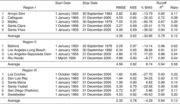
Hydrologic data from five watersheds were extracted from Region I and evaluated against simulated flow from the archetypal watershed (Table 5). Simulations from the Region I archetype provided fair representation of regional watershed behavior. Aver-age statistics (RMSE=4.35 cm; NSE=0.62;R2₌0.79) indicate the model reasonably 15

simulates mean monthly flow behavior, with best performance observed for the smallest watershed system (Arroyo Simi). Overall accuracy is slightly reduced during peak flow months (January–March) when compared to most of the region’s watersheds. Attempts to increase peak discharge behavior for the winter months resulted in consistently higher flows throughout the year and somewhat reduced accuracy in simulating low 20

flow behavior. This also reduced sediment concentrations to below observed ranges. Hence derivation of our final parameters values involved giving appropriate weight to low-flow accuracy while maintaining adequate peak discharge simulation. For Region II, the mean monthly trends (Fig. 3b) closely match overall observations in the region with relatively high NSE (0.82) andR2(0.95). There is slight over-simulation during the 25

(14)

HESSD

9, 13729–13771, 2012

S. R. Lopez et al.

Title Page

Tables Figures

◭ ◮

Back Close

Full Screen / Esc

Discussion

P

a

per

|

Dis

cussion

P

a

per

|

Discussion

P

a

per

|

Discussio

n

P

a

per

|

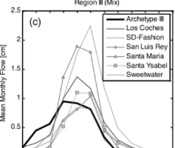
generally within the range of the long-term observations. Overall statistics and visual in-spection indicate model simulations for Region III capture low flow regimes better than in Region I and II (RMSE=2.32 cm) and overall simulations generally reside within the range of flow observations (Table 5). There is a slight under-simulation of peak behav-ior (% BIAS=−4.29), but there is still a strong correlation to observations (R2=0.94)

5

and reasonable overall model performance (NSE=0.78).

Emphasis was placed on capturing annual long-term observations, in addition to monthly streamflow trends. Runoff ratios (annual runoff depth/annual precipitation depth) were calculated for the archetypal watersheds and compared to regional values (Table 5). The runoff ratio provides an estimate of the amount of precipitation leav-10

ing a system as surface flow and how much is lost to other processes (i.e., evapora-tion/evapotranspiration, infiltration, etc.). Region I’s archetype model (vegetated) sim-ulates a relatively low average runoff ratio, 0.11, which is within the observed range for Region I and just above the mean runo_ffratio (0.12). The Malibu and Santa Ynez watersheds have higher runoffratios during years where observed annual precipitation 15

exceeds the mean (approximately 40 cm) (Fig. 3d). A potential reason for this behav-ior may be the amount of urbanization in these watersheds which slightly exceeds the archetype, promoting higher runoffbehavior.

The runoffratio for Region II’s archetypal model is 0.53 due to the higher impervious land cover. The simulated value closely matches the mean observed ratio for the region 20

(0.58). The archetypal model over-simulates in comparison to the Los Angeles sites (Long Beach and Sepulveda Dam; Table 5 and Fig. 3e), especially for events less than the mean annual precipitation (40 cm). However, our simulation does capture the long-term runofftrends of the Rio Hondo and Ballona watersheds, which are physically more similar to our Region II archetype in area (236 and 233 km2, respectively) and urban 25

development (approximately 90 %; Ackerman et al., 2005 and RMC, 2011).

(15)

HESSD

9, 13729–13771, 2012

S. R. Lopez et al.

Title Page

Tables Figures

◭ ◮

Back Close

Full Screen / Esc

Discussion

P

a

per

|

Dis

cussion

P

a

per

|

Discussion

P

a

per

|

Discussio

n

P

a

per

|

follow the fit-line from the archetypal watershed for dry, normal and wet years. Sweet-water River Sweet-watershed experiences higher runoff ratios during wetter years than the model archetype. This is likely due to a much higher urbanization extent (85 %) than the archetypal system (22 %) or flow alterations due to two dams within the lower por-tion of the watershed (Inman and Jenkins, 1999).

5

3.3 Archetypal evaluation: baseline period sediments

The 2nd order rating curves generated from observations within each respective region reside within the 95 % confidence intervals from the archetypal watersheds (Fig. 4). The rating curve from Region III’s archetypal system closely matches the observa-tions; however, sediment comparisons for this region should be interpreted cautiously 10

given there is a limited availability of sediment data. Santa Margarita (1978 WY), San Dieguito (1984 WY) and San Diego-Fashion (1984 WY) streams had only 365 days of available sediment data. Long-term sediment loads from each system were also compared to literature values and found reasonable comparisons.

The mean annual sediment fluxes for the archetypal watersheds are 2.83×106t yr−1,

15

3.66×105t yr−1, 6.13×105t yr−1, for the 50 yr simulation period for Regions I, II and III,

respectively. Sediment observations were unavailable for the entire simulation period, but simulations from each archetype were compared to values produced by Inman and Jenkins (1999; Table 6). Mean annual sediment flux from Region I’s archetypal watershed is higher than the regional average but does reside within the range of ob-20

servations. Similarly, the urban archetypal watershed (Region II) provides a reasonable comparison to sediment observations. This system behaves like an urbanized system with lower annual sediment fluxes in comparison to the other two archetypal systems. Region III’s sediment flux falls within observations, but is higher than the average of the observations. As previously mentioned the lower portion of the Sweetwater River 25

(16)

HESSD

9, 13729–13771, 2012

S. R. Lopez et al.

Title Page

Tables Figures

◭ ◮

Back Close

Full Screen / Esc

Discussion

P

a

per

|

Dis

cussion

P

a

per

|

Discussion

P

a

per

|

Discussio

n

P

a

per

|

(Tables 2 and 3) were then used in each archetypal model to evaluate climate sensitiv-ity as described below.

3.4 Runoffevaluation: temperature increase

Percent deviation in flow (change from observations to simulations) was evaluated dur-ing the baseline period to highlight archetypal system sensitivity to increasdur-ing temper-5

atures. An increase in temperatures lowered overall simulated discharge in all three systems (Fig. 5), but the vegetated and mixed vegetated systems exhibit more sensi-tivity to changes in temperature than the urban archetype. In all systems, the largest loss occurs during the driest months (June–August). Temperature increase alone has minimal effect on peak discharge for all systems. Only the vegetated system experi-10

enced very minor (0–7 %) reductions in peak discharge for low flow events (recurrence interval<20 yr) and no changes to extreme storm events.

Flow loss due to 0.5 and 3◦C temperature increases was estimated by

compar-ing cumulative flow depths for the 50 yr period. Cumulative flow depths for the three archetypal systems are 199, 885 226 cm, for Regions I, II, and III, respectively. The cu-15

mulative flow losses over the 50-yr period due to a 0.5◦C temperature increase are 1.5, 0.9, 0.3 cm for Region I, II, and III’s archetypes, respectively. Cumulative flow losses due to a 3◦_{C increase are 8.4, 5.1, 1.9 cm, respectively. Compared to total flow for} the baseline period, the cumulate flow losses due to a temperature increase are not significant.

20

3.5 Runoffevaluation: temperature increase and precipitation variability

As expected, flow simulations resulting from the combined inputs of precipitation vari-ability and increasing temperature exhibit greater sensitivity than simulations with tem-perature alone. The addition of precipitation variability causes fluctuations in mean monthly flow during the winter and spring periods and temperature increase impacts 25

(17)

HESSD

9, 13729–13771, 2012

S. R. Lopez et al.

Title Page

Tables Figures

◭ ◮

Back Close

Full Screen / Esc

Discussion

P

a

per

|

Dis

cussion

P

a

per

|

Discussion

P

a

per

|

Discussio

n

P

a

per

|

to peak discharge and total annual storm volume. Changes in peak discharge and an-nual storm volume for two return periods that coincide with low flow (2 yr recurrence interval) and high flow (35 yr recurrence interval) points were evaluated within the 50 yr period (Fig. 6). The upper and lower limits of the shaded region primarily correspond to results from the extreme low (5 %) and high (50 %) changes to precipitation variability. 5

Peak discharge for the vegetated archetype showed less sensitivity to precipitation variability than the urban and mixed systems for the 2 yr recurrence interval. The vege-tated archetype experienced a−5 to 17 % deviation (from 22 cm s−1) in peak discharge

(Fig. 6). The deviation ranges for peak discharge were−8 to 32 % (from 590 cm s−1)

for Region II, and−5 to 25 % (from 121 cm s−1) for Region III. These changes in low

10

flow behavior, especially the increase in peak flow, cause a slight shift in the recurrence intervals. Deviation ranges for Region I–III’s archetypal watersheds for the 35 yr recur-rence interval ranged from 4 to 92 % (from 46 cm s−1), 5 to 104 % (from 1817 cm s−1) and 6 to 120 % (from 280 cm s−1

), respectively. The deviations are significant in all sys-tems. The lower end of the deviations in the 35 yr recurrence interval flows are due to 15

only a 5 % precipitation variability and 3◦C temperature increase. The maximum peak discharge deviation (due to 50 % variability and 0.5◦_{C temperature increase) from all} systems results in peak values outside the baseline range.

The 10, 25, 50, 75 and 90 % probability peak flow values in each archetypal sys-tem were identified, then the impact singularly varying precipitation has on peak dis-20

charge was categorized for select recurrence intervals. In the vegetated system, high frequency storms appear more sensitive to 5 and 10 % precipitation variability, further increase in precipitation uncertainty has little e_ffect on peak discharge. The low fre-quency storms in the vegetated system show little deviation in peak discharge due to varying precipitation. The urbanized and mixed systems are predominately governed 25

(18)

HESSD

9, 13729–13771, 2012

S. R. Lopez et al.

Title Page

Tables Figures

◭ ◮

Back Close

Full Screen / Esc

Discussion

P

a

per

|

Dis

cussion

P

a

per

|

Discussion

P

a

per

|

Discussio

n

P

a

per

|

Changes in storm volume response are enhanced in systems with more vegetated land cover. System deviations in total annual storm volume for the 2 yr recurrence in-terval are−7 to 6 % (from 2×1013L),−5 to 3 % (from 1×1014L) and−5 to 11 % (from

3×1013L), for Regions I, II and III, respectively (Fig. 6). The absolute quantity in storm

volume from the vegetated system is less than the urban and mixed systems; however, 5

the percent deviation from baseline is much larger. Evaluating the 35 yr recurrence in-terval, the least extreme climate scenario (5 %, 0.5◦C) caused virtually no change to annual storm volume in all systems. The deviation ranges for Region I, II and III are 0 to 23% (from 1×1014), 0 to 16 % (from 4×1014) and −1 to 32 % from (1×1014),

respectively. 10

3.6 Sediment evaluation: temperature increase

Given the observed sensitivity of low flow regimes, sediment evaluation was focused on daily concentrations and annual storm sediments during low flow periods. Low flows were classified as those with 90 % probability of exceedance using the Weibull proba-bility distribution for each archetype (not shown). As previously discussed, temperature 15

increases are expected to cause a reduction in daily flow during dry periods. This re-sults in an increase in daily suspended sediment concentrations. With projected tem-perature increases of 0.5 and 3◦_{C, the maximum increases in suspended sediment are} 112 % to 600 %, respectively, within the vegetated system and 59 % to 283 % within the mixed archetypal watershed, respectively (Fig. 7a–c). The maximum increase in sus-20

pended sediment due to 0.5 and 3◦_{C temperature increases within the urban system} was 17 % and 38 %, respectively.

Annual storm sediments within the urban archetypal watershed exhibit minor changes with temperature increases (Fig. 7d–f). The 2 yr recurrence interval is altered only−0.3 to 0.2 % (from 9.6×109t) within the urban archetype. The ranges of

devi-25

ation for the 2 yr recurrence interval are −3 to −0.6 % (from 6×1010t) and −1.5 to −0.2 % (from 1.4×1010t), for the vegetated and mixed archetypal watersheds,

(19)

HESSD

9, 13729–13771, 2012

S. R. Lopez et al.

Title Page

Tables Figures

◭ ◮

Back Close

Full Screen / Esc

Discussion

P

a

per

|

Dis

cussion

P

a

per

|

Discussion

P

a

per

|

Discussio

n

P

a

per

|

alter the annual suspended-sediment concentrations in any of the modeled archetypal watersheds.

3.7 Sediment evaluation: temperature increase and precipitation variability

Cumulative distribution functions of annual sediment flux (load per unit time) were examined due to climate variability; extreme (10, 90 % probability) and average 5

(50 % probability) sediment flux from each region were compared. The urban system experienced marginal sensitivity to the climate scenarios during years characterized by low sediment flux at 10 % probability of occurrence. The vegetated and mixed systems, however, show changes in sediment flux from−5 to 8 % and−15 to 46 %, respectively.

The mixed system exhibits a wider deviation because the impervious land cover en-10

hances runoff whereas the pervious land cover provides a sediment source. When

temperature and precipitation changes are combined, both surfaces likely show an in-crease in sediment flux. For an average year, the mixed system again has a wider distribution than the vegetated and urban archetypes. A relative increase in sediment flux of 13 %, 4 % and 34 % was noted for Regions I, II and III, respectively. The years 15

characterized by high sediment flux (90 % probability) caused a larger increase in the urban system by 39 %, than the vegetated (2 %) and mixed (8 %) archetypes.

Finally, long-term changes to annual storm sediment loads (tons) due to temperature increase and precipitation variability were evaluated (Fig. 8). The deviation range for the 2 yr recurrence interval for Regions I, II and III is−8 to 13 % (from 6×1010),−5 to

20

11 % (from 1010) and−7 to 33 % (from 1.4×1010), respectively. Storm sediments from

the vegetated and mixed systems are impacted more than the urban system during low flow periods. As previously discussed, the urban system experienced increased sensi-tivity to peak discharge due to temperature increase and precipitation variability during extreme storm events. Increased wash-offof sediments from the surface is caused by 25

enhanced peak discharge. Annual storm sediment deviations from the 35 yr recurrence interval are 1.3 to 80 % (from 5×1011), 1 to 192 % (from 6.4×1010) and 1 to 116 %

(20)

HESSD

9, 13729–13771, 2012

S. R. Lopez et al.

Title Page

Tables Figures

◭ ◮

Back Close

Full Screen / Esc

Discussion

P

a

per

|

Dis

cussion

P

a

per

|

Discussion

P

a

per

|

Discussio

n

P

a

per

|

4 Discussion

The current study utilized a novel framework based on regional archetypal watersheds to elucidate and quantify potential impacts from climate variability on runoff and sed-iment fluxes in southern California. Regional archetypal watersheds were developed that closely matched observed hydrologic and sediment behavior. Vegetation and ur-5

banization extent heavily influenced sensitivity in future flow and sediment fluxes, as reflected by the three archetypal systems.

Temperature increase only will primarily affect the more vegetated watersheds within southern California, especially during the low flow season. Minimal change was noted for storm volume and peak discharge. The loss in flow is likely due to increased evap-10

otranspiration rates from soil and vegetated surfaces, reducing channel flow in the spring and summertime. During low flow periods (90 % probability of exceedance) there is a significant increase in daily sediment concentration in the vegetated and mixed vegetated-urban systems. Sediment inundation due to temperature increase has been noted in previous studies within the Sierra Nevada Mountains (Hayhoe et 15

al., 2004; Mote et al., 2005), the Colorado River Basin (Gleick and Chalecki, 1999; Christensen et al., 2004; McCabe and Wolock, 2008) and the State Water Project and Central Valley (Vicuna et al., 2007). An increase in suspended-sediment concen-tration is expected to have significant implications for downstream ecosystems. Wet-lands, lagoons and estuaries are reliant on upstream inflow and sediment fluxes. Sea-20

sonal alterations to temperature affect inlet flow, sediment and contaminant concentra-tions, which are important driving factors influencing wetland removal of contaminants (Kadlec and Reddy, 2001).

Combined precipitation variability as well as temperature increase affects all archety-pal watershed’s peak storm discharge and annual flow volumes. Urbanization extent 25

(21)

HESSD

9, 13729–13771, 2012

S. R. Lopez et al.

Title Page

Tables Figures

◭ ◮

Back Close

Full Screen / Esc

Discussion

P

a

per

|

Dis

cussion

P

a

per

|

Discussion

P

a

per

|

Discussio

n

P

a

per

|

system will experience previously categorized high flow events at a lower recurrence interval (i.e. a 17 yr storm may occur at a 10 yr interval due to 50 % precipitation vari-ability and 0.5◦C temperature in Region II) and infrequent storm events with a higher recurrence interval will be more extreme. In response, it is anticipated that an increase

in storm sediments due to enhanced scour and wash-o_ff from pockets of pervious

5

surfaces within an urban environment. Urban expansion is known to have an effect on urban runoff that carries sediment and other hazardous materials such as trash, motor oil, fertilizers, animal waste, etc. (Trimble, 1997; ASCE, 2006; Warrick and Ru-bin, 2007). This was evident in Region III’s mixed archetypal watershed. The vegetation and urban extent with the mixed archetype caused a dual affect: the impervious/urban 10

land cover increased peak discharge and storm volume and the pervious/vegetated land cover provided a sediment source increasing sediment concentrations.

Our work corroborates previous studies, and in addition, provides relative quantifica-tion of change that will result from a range of climate scenarios developed within each region. Given extreme precipitation patterns, the lack of infiltration capacity in highly 15

developed and mixed developed systems may potentially exacerbate flooding hazards and stress the region’s aging infrastructure. The City of Los Angeles Infrastructure Re-port Card states the storm water facilities, including open channels, corrugated metal pipes, vitrified clay pipes and other devices, are currently at a grade C+(A being the best and F being the worst) (Troyan, VB 2003). Approximately 48 % of the system was 20

built 20 to 50 yr ago and assumed to have minimal defects, and 41 % was built 50 to 80 yr ago and assumed to have moderate structural defects (Troyan, VB 2003). In 2003, the City’s storm water system was also noted as deficient in capacity because it could not handle flows generated by a 10 yr storm (Troyan, VB 2003). Given the find-ings from this project, climate variability may significantly challenge the capacity of the 25

(22)

HESSD

9, 13729–13771, 2012

S. R. Lopez et al.

Title Page

Tables Figures

◭ ◮

Back Close

Full Screen / Esc

Discussion

P

a

per

|

Dis

cussion

P

a

per

|

Discussion

P

a

per

|

Discussio

n

P

a

per

|

5 Concluding remarks

The significance of our findings relies on investigating each regional system’s ability to adapt to changes in flow and sediment regimes due to predicted climate variability. The developed archetypal watersheds are meant to investigate and quantifyrelative change based on land-cover and can be scaled to consider specific (real) watershed systems. 5

Precipitation, temperature, geological formation and land cover are key factors that affect runoffand sediment yield (Warrick and Mertes, 2009; Inman and Jenkins, 1999). Our approach allows the user to test regional sensitivity to each factor to determine the expected range of deviation in flow and sediment yield and can be scaled to focus on individual watershed analysis.

10

The methods presented in our study provide an alternative approach to evaluate change in flow and sediment flux due to theoretical future temperature and precipita-tion scenarios across regional scales. By comparing regional simulaprecipita-tions to observa-tions it is possible to validate the usability of our quasi-synthetic systems and provide a reasonable assessment of long-term perturbations to flow and sediment due to vary-15

ing climate. The developed method was tested using synthetic scenarios with potential change estimated from the IPCC or literature; this approach was used to validate the usefulness of the method and can be further explored using other model-based sce-narios.

The developed approach can also be expanded by using other rainfall-runoff mod-20

els, high-resolution land cover datasets, alternative approaches to developing climate scenarios, and altering future land cover. Our purpose was to develop a method that can be used in other regions or for specific watersheds where an extensive dataset (physiological, meteorological, hydrologic, sediment) may not available. The advocated benefits of using the developed archetypal watershed approach include:

25

– User-defined regional classification where users can subcategorize within vege-tated and urban regions.

(23)

HESSD

9, 13729–13771, 2012

S. R. Lopez et al.

Title Page

Tables Figures

◭ ◮

Back Close

Full Screen / Esc

Discussion

P

a

per

|

Dis

cussion

P

a

per

|

Discussion

P

a

per

|

Discussio

n

P

a

per

|

– Significant potential for application to ungauged (non-instrumented) systems.

– Quantification of sediment and streamflow changes that can be used to investi-gate impacts on a range of sensitive downstream ecosystems and infrastructure.

– Ability to investigate multiple climate scenarios with relative ease due to minimal necessary calibration parameters.

5

– Ability to aggregate watershed effects to look for regional patterns and potential effects on specific coastal systems, including the southern California Bight.

Future work includes investigating potential environment effects on downstream estu-aries due to changing hydrologic and sediment fluxes. Additional work is likely needed to assess the impacts of climate change on nutrient and metal transport from coastal 10

watersheds to downstream aquatic ecosystems. Future analysis will also focus on changes in extent and distribution of aquatic ecosystems due to changes in terrestrial (flow, sediment, contaminants) as well as oceanic forcing (salt-water intrusion).

Acknowledgements. This work was primarily funded by the California State Water Board (#06– 241–250), the Southern California Coastal Water Research Project (SCCWRP) and a Na-15

tional Science Foundation Graduate Research Fellowship (DGE #0707424). Special thanks to Drew Ackerman for guidance on the HSPF modeling for this project and to Eric Stein for co-authoring this submitted publication.

References

Ackerman, D., Schiff, K. C., and Weisberg, S. B.: Evaluating HSPF in an Arid, Urbanized

Wa-20

tershed, J. Am. Water. Resour. As., 41, 477–486, 2005.

(24)

HESSD

9, 13729–13771, 2012

S. R. Lopez et al.

Title Page

Tables Figures

◭ ◮

Back Close

Full Screen / Esc

Discussion

P

a

per

|

Dis

cussion

P

a

per

|

Discussion

P

a

per

|

Discussio

n

P

a

per

|

American Society of Civil Engineers (ASCE): California Infrastructure Report Card: A Cit-izen’s Guide (available at: http://www.ascecareportcard.org/Citizen guides/2006 citizens guide.pdf), 2006.

Bandurraga, M., Rindahl, B., and Butcher, J.: Use of HSPF for Design Storm Modeling in Semi-Arid Watersheds, ASCE Conference Proceedings, 414, 4579–4586, 2011.

5

Bicknell, B., Imhoff, J. C., Kittle, J. L., Jobes, T. H., and Donigian, A. S.: Hydrological

Simula-tion Program–Fortran (HSPF): User’s Manual for Release 12, US Environmental ProtecSimula-tion Agency: Athens, GA, 2000.

California Climate Change Center (CCCC): Our Changing Climate–Assessing the Risks to Cal-ifornia, available at:http://www.climatechange.ca.gov/biennial reports/2006report/index.html 10

(last access: 15 November 2007), 2006.

California Department of Conservation–Division of Land Resource Protection: Farmland Map-ping and Monitoring Program, available at: http://redirect.conservation.ca.gov/DLRP/fmmp/ county info results.asp, 2011.

California Department of Finance: Population Projections for California and Its Counties 2000– 15

2050, by Age, Gender and Race/Ethnicity, Sacramento, California, July 2007, 2007.

Christensen, N. S., Wood, A. W., Voisin, N., Lettenmaier, D. P., and Palmer, R. N.: The Effects

of Climate Change on the Hydrology and Water Resources of the Colorado River Basin, Climatic Change, 62, 337–363, 2004.

Clark, G. M.: Changes in Patterns of Streamflow from Unregulated Watersheds in Idaho, West-20

ern Wyoming, and Northern Nevada, J. Am. Water. Resour. As., 46, 486–497, 2010.

Climate action team (CAT): Biennial Report, March 2009, available at: http://www.energy.ca. gov/2009publications/CAT-1000-2009-003/CAT-1000-2009-003-D.PDF (last access: 10 Oc-tober 2010), 2009.

Costa, A. C. and Soares, A.: Trends in extreme precipitation indices derived from a daily rainfall 25

database for the South of Portugal, Int. J. Climatol., 29, 1956–1975, 2009.

Department of Water Resources (DWR): Climate Change Report–Progress on Incorporating Climate Change into Management of California’s Water Resources Technical Memorandum

Report, available at: http://baydeltao_ffice.water.ca.gov/climatechange.cfm (last access: 16

January 2010), 2006. 30

DeWalle, D. R., Swistock, B. R., Johnson, T. E., and Maguire, K. J.: Potential Effects of Climate

(25)

HESSD

9, 13729–13771, 2012

S. R. Lopez et al.

Title Page

Tables Figures

◭ ◮

Back Close

Full Screen / Esc

Discussion

P

a

per

|

Dis

cussion

P

a

per

|

Discussion

P

a

per

|

Discussio

n

P

a

per

|

Donigian, A. S. and Love, J. T.: Sediment Calibration Procedures and Guidelines for Watershed Modeling, Water Environment Federation, 20, 728–747, 2003.

Fall, S., Niyogi, D., Gluhovsky, A., Roger, A., and Pielke, S.: Impacts of land use land cover on temperature trends over the continental United States: Assessment using the North Ameri-can Regional Analysis, Int. J. Climatol., 30, 1980–1993, 2010.

5

Fowler, H. J., Blenkinsop, S., and Tebaldi, C.: Linking climate change modeling to impacts stud-ies: recent advances in downscaling techniques for hydrological modeling, Int. J. Climatol., 27, 1547–1578, 2007.

Githui, F., Gitau, W., Mutua, F., and Bauwens, W.: Climate change impact on SWAT simulated streamflow in western Kenya, Int. J. Climatol., 29, 1823–1834, doi:10.1002/joc.1828, 2009. 10

Gleick, P. H. and Chalecki, E. L.: The Impacts of Climate Changes for Water Resources of the Colorado and Sacramento–San Joaquin River Basins, J. Am. Water Resour. As., 35, 1429–1441, 1999.

Hack, J. T.: Studies of Longitudinal Profiles in Virginia and Maryland, US Geological Survey Professional Papers, Vol. 294-B, 45–97, 1957.

15

Hayhoe, K., Cayan, D., Field, C. B., Frumhoff, P. C., Maurer, E. P., Miller, N. L., Moser, S.

C., Schneider, S. H., Cahill, K. N., Cleland, E. E., Dale, L., Drapek, R., Hanemann, R. M., Kalkstein, L. S., Lenihan, J., Lunch, C. K., Neilson, R. P., Sheridan, S. C., and Verville, J. H.: Emissions Pathways, Climate Change, and Impacts on California, P. Natl. Acad. Sci. USA, 101, 12422–12427, 2004.

20

He, M. and Hogue, T. S.: Integrating Hydrologic Modeling and Land Use Projections for Evalua-tion of Hydrologic Response and Regional Water Supply Impacts in Semi-arid Environments, Environmental Earth Sciences, 65, 1671–1685, 2011.

Hertig, E. and Jacobeit, J.: Assessments of Mediterranean precipitation changes for the 21st century using statistical downscaling techniques, Int. J. Climatol., 28, 1025–1045, 2008. 25

Hevesi, J. A., Flint, L. E., Church, C. D., and Mendez, G. O.: Application of a watershed model (HSPF) for evaluating sources and transport of pathogen indicators in the Chino Basin drainage area, San Bernardino County, California, US Geological Survey Scientific Inves-tigations Report, 2009–5219, p. 146 , 2011.

Hidalgo, H. G., Das, T., Dettinger, M. D., Cayan, D. R., Pierce, D. W., Barnett, T. P., Bala, G., 30

(26)

HESSD

9, 13729–13771, 2012

S. R. Lopez et al.

Title Page

Tables Figures

◭ ◮

Back Close

Full Screen / Esc

Discussion

P

a

per

|

Dis

cussion

P

a

per

|

Discussion

P

a

per

|

Discussio

n

P

a

per

|

Inman, D. and Jenkins, S.: Climate: Change and the Episodicity of Sediment Flux of Small California Rivers, J. Geology, 107, 251–270, 1999.

Intergovernmental Panel on climate Change (IPCC): Climate Change 2001, Special Report on Emission Scenarios, edited by: Nakicenovic, N. and Swart, R., Contribution of Working Group I to the Third Assessment Report of the Intergovernmental Panel on Climate Change, 5

Cambridge University Press, Cambridge United Kingdom and New York, NY, USA, 2001. Intergovernmental Panel on climate Change (IPCC): Climate Change 2007: Synthesis Report,

Contribution of Working Groups I, II and III to the Fourth Assessment Report of the Inter-governmental Panel on Climate Change, edited by: Core Writing Team, Pachauri, R. K., and Reisinger, A., IPCC, Geneva, Switzerland, 104 pp., 2007.

10

Kadlec, R. H. and Reddy, K. R.: Temperature Effects in Treatment Wetlands Water Environment

Research, Water Environment Federation, 73, 543–557, 2001.

Kim, J.: A projection of the e_ffects of climate change induced by increased CO₂ on extreme

hydrologic events in the western US, Climatic Change, 68, 153–168, 2005.

Kiparsky, M. and Gleick, P. H.: Climate Change and California Water Resources: A Survey and 15

Summary of the Literature, Pacific Institute for Studies in Development, Environment, and Security, Oakland, CA, 2003.

Knowles, N. and Cayan, D. R.: Potential Effects of Global Warming on the Sacramento/San

Joaquin Watershed and the San Francisco Estuary, Geophys. Res. Lett., 29, 381–384, 2002. Kunkel, K. E., Palecki, M., Ensor, L., Hubbard, K. G., Robinson, D., Redmond, K., and Easter-20

ling, D.: Trends in twentieth-century US snowfall using a quality-controlled dataset, J. Atmos. Ocean. Tech., 26, 33–44, 2009.

Levien, L., Fischer, C., Parks, S., Maurizi, B., Suero, J., Mahon, L., Longmire, P., and Roffers, P.:

Monitoring land cover changes in California, a USFS and CDF cooperative program, South Coast Project Area, State of California, Resources Agency, Department of Forestry and Fire 25

Protection, Sacramento, CA, 2002.

Lutz, K., Jacobeit, J., Philipp, A., and Seubert, S.: Comparison and evaluation of statistical downscaling techniques for station-based precipitation in the Middle East, Int. J. Climatol., 32, 1579–1595, 2011.

Maurer, E. P. and Hidalgo, H. G.: Utility of daily vs. monthly large-scale climate data: an inter-30

(27)

HESSD

9, 13729–13771, 2012

S. R. Lopez et al.

Title Page

Tables Figures

◭ ◮

Back Close

Full Screen / Esc

Discussion

P

a

per

|

Dis

cussion

P

a

per

|

Discussion

P

a

per

|

Discussio

n

P

a

per

|

Meehl, G. A., Zwiers, F., Evans, J., Knutson, T., Mearns, L., and Whetton, P.: Trends in extreme weather and climate events: issues related to modeling extremes in projections of future climate change, B. Am. Meterol. Soc., 81, 427–436, 2000.

McCabe, G. J. and Wolock, D. M.: Warming and Implications for Water Supply in the Col-orado River Basin, In World Environmental and Water Resources Congress 2008: Ahupua’a, 5

ASCE, 273, 1–10, 2008.

Miller, N. L., Bashford, K. E., and Strem, E.: Potential impacts of climate change on California hydrology, J. Am. Water. Resour. As., 39, 771–784, 2003.

Mote, P. W., Hamlet, A. F., Clark, M. P., and Lettenmaier, D. P.: Declining mountain snowpack in western North America, B. Am. Meterol. Soc., 86, 39–49, 2005.

10

National Oceanographic and Atmospheric Administration-Coastal Services Center (NOAA-CSC): Southern California 2000-Era Land Cover/Land Use, LANDSAT-TM, 30 m, NOAA– CSC, Charleston, SC, available at: http://www.csc.noaa.gov/crs/lca/pacificcoast.html (last access: 1 July 2007), 2003.

National Oceanographic and Atmospheric Administration – National Weather Service (NOAA-15

NWS): Climate Prediction Center Cold and Warm Episodes by Season, available at: http://

www.cpc.noaa.gov/products/analysis monitoring/ensostuff/ensoyears.shtml (last access: 20

December 2010), 2010.

Nearing, M. A., Jetten, V., Baffaut, C., Cerdan, O., Couturier, A., Hernandez, M., Le Bissonnais.

Y., Nichols, M. H., Nunes, J. P., Renschler, C. S., Souchere, V., and van Oost, K.: Modeling 20

response of soil erosion and runoffto changes in precipitation and cover, Catena, 61, 131–

154, 2005.

Nezlin, N. P. and Stein, E. D.: Spatial and temporal patterns of remotely-sensed and field-measured rainfall in southern California, Remote Sens. Environ., 96, 228–245, 2005. Payne, J. T., Wood, A. W., Hamlet, A. F., Palmer, R. N., and Lettenmaier, D. P.: Mitigating the 25

Effects of Climate Change on the Water Resources of the Columbia River Basin, Climatic

Change, 62, 233–256, 2004.

Philips, J. R.: The theory of infiltration: the infiltration equation and its solution, Soil Sci., 83, 345–375, 1957.

Pruski, F. F. and Nearing, M. A.: Climate-induced changes in erosion during the 21st century 30

for eight US locations, Water Resour. Res., 38, 1298–1309, 2002.

Randhir, T.: Watershed-scale effects of urbanization on sediment export: Assessment and