www.geosci-model-dev.net/10/333/2017/ doi:10.5194/gmd-10-333-2017
© Author(s) 2017. CC Attribution 3.0 License.
Process-based modelling of the methane balance in periglacial
landscapes (JSBACH-methane)
Sonja Kaiser1, Mathias Göckede1, Karel Castro-Morales1, Christian Knoblauch2, Altug Ekici1,3, Thomas Kleinen4, Sebastian Zubrzycki2, Torsten Sachs5, Christian Wille2, and Christian Beer6,7
1Max Planck Institute for Biogeochemistry, Jena, Germany
2Department of Earth Sciences, Universität Hamburg, Hamburg, Germany 3Uni Research Climate, Bjerknes Centre for Climate Research, Bergen, Norway 4Max Planck Institute for Meteorology, Hamburg, Germany
5Helmholtz Centre Potsdam GFZ German Research Centre for Geosciences, Potsdam, Germany
6Department of Environmental Science and Analytical Chemistry (ACES), Stockholm University, Stockholm, Sweden 7Bolin Centre for Climate Research, Stockholm University, Stockholm, Sweden
Correspondence to:Sonja Kaiser ([email protected]) and Mathias Göckede ([email protected])
Received: 28 April 2016 – Published in Geosci. Model Dev. Discuss.: 2 June 2016 Revised: 27 October 2016 – Accepted: 5 December 2016 – Published: 24 January 2017
Abstract. A detailed process-based methane module for a global land surface scheme has been developed which is gen-eral enough to be applied in permafrost regions as well as wetlands outside permafrost areas. Methane production, ox-idation and transport by ebullition, diffusion and plants are represented. In this model, oxygen has been explicitly in-corporated into diffusion, transport by plants and two oxi-dation processes, of which one uses soil oxygen, while the other uses oxygen that is available via roots. Permafrost and wetland soils show special behaviour, such as variable soil pore space due to freezing and thawing or water table depths due to changing soil water content. This has been integrated directly into the methane-related processes. A detailed ap-plication at the Samoylov polygonal tundra site, Lena River Delta, Russia, is used for evaluation purposes. The applica-tion at Samoylov also shows differences in the importance of the several transport processes and in the methane dynam-ics under varying soil moisture, ice and temperature condi-tions during different seasons and on different microsites. These microsites are the elevated moist polygonal rim and the depressed wet polygonal centre. The evaluation shows sufficiently good agreement with field observations despite the fact that the module has not been specifically calibrated to these data. This methane module is designed such that the advanced land surface scheme is able to model recent and future methane fluxes from periglacial landscapes across
scales. In addition, the methane contribution to carbon cycle– climate feedback mechanisms can be quantified when run-ning coupled to an atmospheric model.
1 Introduction
forcing from all greenhouse gases. Thus, for the radiation balance and the chemistry of the atmosphere, it is important to understand land–atmosphere exchanges of methane.
Environmental conditions are highly heterogeneous in per-mafrost regions, where landscapes are often characterised by small-scale mosaics of wet and dry surfaces (Sachs et al., 2008). The heterogeneous aerobic and anaerobic condi-tions in permafrost soils, in concert with elevated soil carbon stocks (Hugelius et al., 2014), set the conditions for large and spatially heterogeneous methane emissions in these ar-eas (Schneider et al., 2009). Such strongly varying environ-mental and soil conditions as well as processes that influence the methane production and emissions are challenges in a process-based model with a bottom-up approach for methane balance estimation, simply because of the complexity of the network of processes to consider as well as their unclear in-teractions.
However, process-based modelling approaches are pow-erful tools that help to quantify recent and future methane fluxes on a large spatial scale and over long time periods in such remote areas. They can give first estimates of where field measurements are missing and help to understand the effects of climate change on permafrost methane emissions. In addition, the effect of methane emissions on climate, and hence feedback mechanisms, can be analysed using an Earth system model. For such purposes, a methane module for an Earth system model has to be process-based and working un-der most environmental conditions, including permafrost.
Currently existing process-based methane models have usually been developed for applications in temperate or trop-ical wetlands, without considering permafrost-specific bio-geophysical processes, such as e.g. freezing and thawing soil processes (e.g. Zhu et al., 2014; Schuldt et al., 2013). In other cases, they are embedded within a vegetation model, which cannot easily be coupled to an atmospheric model (e.g. Schaefer et al., 2011; Wania et al., 2010; Zhuang et al., 2004). Some models have been developed only for small-scale applications (e.g. Xu et al., 2015; Mi et al., 2014; Khvorostyanov et al., 2008; Walter and Heimann, 2000) or use an empirical approach (e.g. Riley et al., 2011). Highly simplified models might be less reliable for global applica-tions (e.g. Jansson and Karlberg, 2011; Christensen et al., 1996) because of oversimplification in simulating the com-plexity of the methane processes.
The aim of this study is to introduce a new methane mod-ule that is running as part of a land surface scheme of an Earth system model. Moreover, it shall be general enough for global applications, including terrestrial permafrost ecosys-tems. The methane module presented in this work represents the gas production, oxidation and relevant transport pro-cesses in a process-based fashion. Among other propro-cesses, this new methane module takes into account the size vari-ation of the pore spaces in the soil column in relvari-ation to the freezing and thawing cycles, influencing directly the methane concentration in the soil. Furthermore, in this module the
oxygen content is explicitly taken into account, enabling two process-based oxidation processes: bulk soil methane oxida-tion and rhizospheric methane oxidaoxida-tion.
The platform chosen to develop the methane module is the JSBACH (Jena Scheme for Biosphere Atmosphere Coupling in Hamburg) land surface scheme of the MPI-ESM (Max Planck Institute Earth System Model). The starting point was a model version that has a carbon balance (Reick et al., 2013) and a five-layer hydrology (Hagemann and Stacke, 2015) and that includes permafrost as described in Ekici et al. (2014). A parallel development by Schuldt et al. (2013) incorpo-rated wetland carbon cycle dynamics and was also integincorpo-rated into the model version presented in this work. The bases for the methane-related processes were the works by Walter and Heimann (2000) and Wania et al. (2010). Special focus was also placed on the connections with permafrost and wetland as well as the explicit consideration of oxygen. This paper describes the newly developed methane module, and, for the purpose of model evaluation, it presents an application at a typical polygonal tundra site in the north of the Sakha (Yaku-tia) Republic, Russia.
2 Methods
2.1 Site description
For the purpose of evaluation, this model has been applied at the Samoylov island site, located 120 km south of the Arctic Ocean in the Lena River Delta in Yakutia, with an elevation of 10 to 16 m above sea level. The mesorelief of Samoylov is flat, while as microrelief, there are low-centre polygons with the soil surface about 0.5 m higher at the rim than at the centre. This results in different hydrological conditions also influencing heat conduction. The average maximum ac-tive layer depth at the dryer but still moist polygonal rims and the wet polygonal centres is about 0.5 m (Boike et al., 2013). While the water table at the polygonal rims is gen-erally well below the soil surface, the polygonal centres are often water-saturated, with water tables at or above the soil surface (Sachs et al., 2008).
site. Below, moist microsites will be referred to as rim and wet microsites as centre.
2.2 Methane module description 2.2.1 Layer structure
For a numerically stable representation of gas transport pro-cesses in soils, a much finer vertical soil structure is required than what is normally used for thermal and hydrological pro-cesses in JSBACH. Therefore, a new soil layering scheme has been implemented for the methane module. This scheme is variable and allows fine layers (of the order of a few cen-timetres), but still inherits the hydrological and thermal in-formation contained in the coarse scheme. The number and height of layers can be chosen arbitrarily, also allowing non-equidistant solutions.
Internally, the module uses midpoints and lower bound-aries of the layers as well as distances between midpoints. At the bottom, the layering scheme is truncated at depth to bedrock. The layers where
– the plant roots end, i.e. the rooting depth lies, – the water table lies and
– the minimum daily water table over the previous year lies (permanent saturated depth)
have also been determined. These layers have a specific func-tion for methane producfunc-tion and various transport processes. Details will be given below in the respective sections (see also Appendix A1).
For model evaluation, fine layers with a height of 10 cm have been used. For all the layers of the new soil layering scheme, the soil temperature is interpolated linearly from the coarse JSBACH layering scheme. From these values, the pre-vious day’s mean soil temperature is also calculated. In addi-tion to geometry and soil temperature, each layer has its own hydrological parameters, as described in the next section, and various state variables describing the different gases’ concen-trations.
2.2.2 Hydrology
For the fine layers, several hydrological values have to be determined using the relative soil moisture and ice content from the coarse JSBACH layering scheme. Fine-scale layer values are derived such that known values at common layers are kept and only those layers that span more than one input layer get values of the weighted mean of the involved coarse-layer values. The relative soil water content is then defined by the sum of the relative soil moisture and ice content.
Subtracting the relative ice content from the volumetric soil porosity leads to the ice-corrected volumetric soil poros-ity. With this, the relative moisture content of the ice-free pores can be defined, which is calculated by division of the
relative soil moisture content by the ice-corrected volumetric soil porosity. Finally, the relative air content of the ice-free pores is defined as 1 minus the relative moisture content of the ice-free pores.
The water table is calculated following Stieglitz et al. (1997). From the uppermost soil layer, the water table is lo-cated in the immediate layer above the first one with a relative soil water content of at least 90 % of field capacity. This defi-nition was used because the current hydrology scheme in JS-BACH does not allow one to consider water content of soils higher than field capacity or standing water (Hagemann and Stacke, 2015). Instead, water content exceeding field capac-ity is removed by runoff and drainage. In this context, the cur-rent model implementation considers only mineral soil (field capacity: 0.435; porosity: 0.448); i.e. no peat layers exist in this version. The dimensionless but ice-uncorrected field ca-pacity is used because the relative soil water content already includes ice. The water table depth is then defined as
w=
b, ifrw≤0.7·fc
b−rw−0.7·fc
fc −0.7·fc·h, ifrw>0.7·fc.
(1)
Here,bis the lower boundary of the soil layer of interest with heighthand relative soil water contentrw. fc is the field
ca-pacity. If even the uppermost layer has a relative soil water content of at least 90 % field capacity, the water table is lo-cated at the surface. The mean water table of the previous day is used where appropriate to keep consistency with the daily time step of the carbon decomposition routine. The minimum of this daily mean water table over the previous 365 days is used as the permanently saturated depth.
At a given time step, the soil column, which contains the water table depth and the permanently saturated depth, is di-vided into three strata that are, from the top,
– the unsaturated zone above the water table,
– the saturated zone below the water table (located above the annual minimum water table depth) and
– the permanently saturated zone (located below the an-nual minimum water table depth).
Evidently, this stratification is hydrological, while the lay-ering scheme is purely numerical. Thus, each stratum may contain several soil layers. For carbon decomposition, the mean temperatures of the previous day at the midpoints of these three strata are needed. These values are derived analo-gously to the temperatures in the fine layers by interpolating the mean temperatures of the previous day linearly.
2.2.3 Production
Initial values of methane and oxygen concentrations have been derived using reported gas concentrations in free air for oxygen and methane. For oxygen, the global mean value for 2012 is used (8.56 mol m−3, http://cdiac.ornl.gov/ tracegases.html). The value for methane is defined as the March 2012 value (77.06 µmol m−3, http://agage.eas.gatech. edu/data.htm).
The initial gas concentrations in the soil profile are deter-mined assuming equilibrium condition between free ambient air as well as the air and moisture in the soil pore space. Thus, Henry’s law with the dimensionless Henry constant is applied. The dimensionless Henry constant is defined as the ratio of the concentration of gas in moisture to its concentration in air (Sander, 1999). The chosen temperature dependence values, which are d(lnkH CH4) d(T−1)
−1 = 1900 K and d(lnkH O2) d(T
−1)−1
=1700 K, as well as the Henry constants at standard tempera-ture, which are k25H CH4=0.0013 mol dm−3atm−1 and kH O25
2=0.0013 mol dm
−3atm−1, are all from Dean (1992).
The calculated initial values for methane and oxygen con-centrations in the soil profile can be transformed into gas amounts and vice versa. During methane transport process calculation, concentration values are widely used. In between time steps, however, the volume of ice is recalculated and therefore the relative ice-free pore volume changes. Thus, concentration values also change, but only the gas amounts stay constant. Therefore, at the beginning of each methane module execution, the total gas amounts that have been saved at the end of the previous time step are divided by the current relative ice-free pore volume to recalculate the current con-centration values.
The final products of the decomposition of soil carbon are carbon dioxide and methane. Depending on the soil hydro-logical conditions, carbon dioxide or methane are produced from the decomposing carbon pools that belong to the three strata described above. These decomposition results are dis-tributed over fine-scale layers of the whole soil column. Be-cause no direct vertical information about the amount of de-composing carbon is available, equal decomposition velocity in all layers of one stratum is assumed. Thus, once the composed amount of carbon per stratum is known, the de-composed amount of carbon per layer per stratum depends on the amount of available carbon in that layer only. And the carbon content in the soil layers for Samoylov has been prescribed from measurements by Zubrzycki et al. (2013), Harden et al. (2012) and Schirrmeister et al. (2011), taking local horizontal variations of polygonal ground (Sachs et al., 2010) into account (see Appendix A3).
The initial amount of carbon in the pools is obtained from the sum of carbon in each layer of the strata. In this case, the first and second strata share one carbon pool which is split after calculation of the mean water table over the previous
day. The amount of carbon per layer is divided by the amount of carbon per stratum. These weights are used for distributing the amounts of decomposed carbon from strata to layers. In addition, the share of initially produced carbon dioxide and methane is set assuming all decomposed carbon above the water table and half of it below the water table get carbon dioxide:
cCH4 prod=0.5·
fC
P
slfC
· Cs h·vp
. (2)
Here, sl means all layers in the stratum, andCsis the
decom-posed carbon in the stratum.fCis the soil carbon content of
the layer with heighth, andvpis the ice-corrected volumetric
soil porosity. Mass conservation is done if the stratum is too small to get a layer assigned, so that the associated carbon is not neglected. The gas fluxes for methane and carbon diox-ide are calculated via the sums of the respective amounts, and the produced gases are added to their respective pools in the layers.
2.2.4 Bulk soil methane oxidation
Only part of the oxygen in the soil is assumed to be avail-able for methane oxidation. In layers above the mean water table over the previous day, available oxygen is reduced by the amount that corresponds to the amount of carbon dioxide which is produced by heterotrophic respiration but not more than 40 % of the total oxygen content. An additional 10 % of oxygen is assumed to be unavailable and also reduced. In lay-ers below the water table, the amount of oxygen is reduced by 50 %. This approach is similar to Wania et al. (2010).
For methane oxidation itself, a Michaelis–Menten kinetics model is applied. The Q10 temperature coefficient is
sim-ilar to the one used by Walter and Heimann (2000), but with a reference temperature of 10◦C rather than the annual
mean soil temperature. Reaction velocities of both, methane and oxygen, are taken into account by using an additional equivalent term with the concentration of oxygen andKO2
m =
2 mol m−3, which is chosen to be the average concentration of oxygen at the water table. Furthermore, methane and oxy-gen follow a prescribed stoichiometry:
cCH4 oxid =min
Vmax·
cCH4 KCH4
m +cCH4
· c
O2
KO2 m +cO2
(3)
·Q
T−10 10
10 ·dt, 2·c
O2, cCH4
.
2.2.5 Ebullition
The implementation of the ebullition of methane largely fol-lows the scheme from Wania (2007). Ebullition is the trans-port of gas via bubbles that form in liquid water within the soil and transport methane rapidly from their place of ori-gin to the water table. The amount of methane to be re-leased through ebullition is determined by that amount of the present methane that can be solute in the present liquid wa-ter. This amount depends on the overall amount of methane present in the layer, but also on the storage capacity of the present liquid water.
In a first step, the concentration of methane in soil air is as-sumed to be in equilibrium with the concentration in soil wa-ter. Thus, by application of Henry’s law, the present methane can be partitioned into the potentially ebullited methane centration in soil air and the potentially solute methane con-centration in soil water. The dimensionless Henry solubili-ties at current soil temperature conditions are used for this. As an initial approximation, all methane is assumed to be in soil air and potentially ebullited. Thus, first, the potentially solute methane in soil water can be determined, but it will also be overestimated because of this approximation. There-fore, second, an updated potentially ebullited concentration of methane in soil air is determined by subtracting the po-tentially solute methane from the total methane. Unlike what was proposed in Wania (2007), these two steps are iterated until stable-state conditions are reached.
In a second step, to calculate the maximal amount of methane that can be soluble in the present soil water, the Bunsen solubility coefficient from Yamamoto et al. (1976) is applied. By considering the available pore volume, this gives the volume of methane that can maximally be dissolved. The ideal gas law results in the maximally soluble amount of methane. For that, the soil water pressure in layers below the water table needs to be derived. This is determined from soil air pressure and the pressure of the water column, using the basic equation of hydrostatics. For this, the specific gas con-stant of moist air and the soil air pressure in layers above the water table are required. For the air pressure calculation, the barometric formula is used. Hereby, the first layer uses the air pressure at the soil surface and deeper layers use the above layer’s soil air pressure. The specific gas constant of moist air finally needs the saturation vapour pressure and relative soil air moisture, both in layers above the water table. The former is calculated following Sonntag and Heinze (1982), and the latter is set to 1 if the relative water content is at least at the wilting point and to 0.9 elsewhere.
Now, the maximally soluble concentration of methane is derived by dividing the maximally soluble amount of methane by the available pore volume. Thus, the concen-tration of methane that is solute and in equilibrium with methane in the air is the lesser of the following two concen-trations: the potentially solute methane that was calculated in the first step, and the maximally soluble methane that was
calculated in the second step. Finally, the actually ebullited methane is the difference between all methane and solute methane,
cebulCH4 =cCH4−min
kH CH4·c CH4 gas ,
β·pw R·T
, (4)
withkHCH4 being the Henry solubility, c CH4
gas the methane
concentration that can potentially be ebullited,β the Bun-sen solubility coefficient,pw the soil water pressure andT
the soil temperature. All these variables relate to the layer, andRis the gas constant.
The ebullited methane is removed from the layers and, if the water table is below the surface, added to the first layer above the water table. In this case, the ebullition flux to at-mosphere is zero, and the methane is still subject to other transport or oxidation processes in the soil. Otherwise, if the water table is at the surface and if snow is not hindering, it is added to the flux to atmosphere. Snow is assumed not to hin-der if snow depth is less than 5 cm. If, finally, the water table is at the surface but snow is hindering, ebullited methane is put into the first layer and the ebullition flux to atmosphere is zero like in the first case.
2.2.6 Diffusion
For the diffusion of methane and oxygen, Fick’s second law with variable diffusion coefficients is applied. The possibil-ity of a non-equidistant layering scheme is specifically taken into account. Diffusion is a molecular motion due to a con-centration gradient, with a net flux from high to low concen-trations. For soil as a porous medium, moreover with chang-ing pore volumes because of different contents of ice, the ice-corrected soil porosity of the layers also has to be accounted for in the equation system directly as a factor (Schikora, 2012). The discretisation of the computational system is done with the Crank–Nicholson scheme with weighted harmonic means for the diffusion coefficients. While ice is treated as non-permeable for gases, the diffusion is allowed to continue if the soil is frozen but not at field capacity; i.e. there is no simple cut at 0◦C. During every model time step of 1 h, two half-hourly diffusion steps are calculated to prevent instabil-ities like oscillations or unrealistic behaviour like negative concentrations. The diffusion-specific time step can be de-creased further if necessary and if an adjustment of the lay-ering scheme is not desired. The possibility of these effects results from the tight connection between layering scheme, time step and diffusion coefficients.
con-ditions are assumed to hold at the boundary, and therefore a Dirichlet type with a gas concentration in free air is applied:
vp·∂c ∂t =
∂ ∂x
D·∂c
∂x
; c=cair, x∈ŴD; (5) ∂c
∂x =0, x∈ŴN .
Here, vp is the volumetric soil porosity, c denotes the gas concentration, t is the time, x is the depth, D denotes the diffusion coefficient,ŴDis the boundary with Dirichlet type
boundary conditions andŴNis the boundary with Neumann
type boundary conditions. For details on how the diffusion coefficients are determined, see Appendix A4. The solu-tion of the diffusion equasolu-tion system is obtained by the tridag_serandtridag_parroutines from Press et al. (1996) in Numerical Recipes.
By subtracting the gas concentrations after diffusion from those before for methane and vice versa for oxygen, con-centration changes are derived with positive values for lost methane and gained oxygen. Multiplying the concentration changes by their respective pore volumes as usual and sum-ming the resulting amounts over the layers gives the total fluxes of methane and oxygen.
2.2.7 Plant transport
Gas transport via plants is first calculated for oxygen entering the soil. Then, another oxidation mechanism with this newly gained oxygen takes place (see Sect. 2.2.8). After that, the transport of methane via plants is modelled. The transport via plants happens through the plant tissue that contains big air-filled channels, the aerenchyma, to foster aeration of the plant’s roots. However, because plants need the oxygen that reaches their roots for themselves, their root exodermis acts as an efficient barrier against gas exchange.
In this model configuration, gas transport by plants is as-sumed to happen only via the phenology type grass with a C3 photosynthetic pathway. The contribution to methane emis-sions due to the degradation of labile root exudates is not taken into account here. The potential role of this process is reviewed in the discussion section. Furthermore, the gas transport via plants will occur only if snow is not hinder-ing, i.e. if there are less than 5 cm of snow. This is justified by the consideration of snow crinkling the culms such that transport is not possible anymore. A diffusion process from aerenchyma through the root tissue to soil is assumed as a key process, and it is described by Fick’s first law. Gas transport is fast inside the air-filled aerenchyma; hence, atmospheric air conditions can be assumed there.
The diffusion flux via the plants is determined from the oxygen concentration gradient between ambient air and the root zone soil layers. The diffusion coefficients of methane and oxygen in the exodermis are unknown but can be as-sumed to be slightly lower than in water (e.g. Kutzbach et al., 2004; Konˇcalová, 1990). Therefore, their values are set
to be 80 % of their respective values in soil water at the given soil temperatures and pressures,Dr=0.8·Dw.
The oxygen flux entering the soil is furthermore con-strained by the surface area of root tissue, Agesr =Ar·qp,
which is determined from the surface area of a single plant’s roots,Ar=lr·dr·π, multiplied by plant density, qp=
tph tp.
Here,lris the root length,drthe root diameter, both in
me-tres,tphthe number of tillers per square metre depending on
phenology andtpthe number of tillers per plant. Finally, the
number of tillers per square metre is influenced by plant phe-nology, which is determined from the leaf area index (LAI), usingtph=max(tm)·maxLAI(LAI), withtmbeing the number of
tillers per square metre. Please also see Appendix A5. The root tissue is assumed to be distributed equally be-tween all root-containing layers; thus,Arlr =Agesr ·Ph
rlh, with hdenoting the layer height and rl all layers with roots. The travel distance, dx, is set to the thickness of the exodermis in metres because this is the limiting factor. The plant transport per layer is thus modelled as
nO2 plant=D
O2 r ·
cO2
air−c O2
· 1
dx ·dt·A rl
r . (6)
Here,cairO2is the concentration of oxygen in free air and dtthe time step length. For every soil layer, the resulting amount of oxygen is converted into concentration and added to the oxygen pool. As usual, the flux of oxygen into the soil is calculated by the total soil column balance.
After plant transport of oxygen, additional methane can be oxidised by the amount of oxygen that leaves the roots (Sect. 2.2.8). The remaining methane is then available for plant transport, which is modelled exactly as for oxygen, with one exception: it is necessary to account for the fraction of roots able to transport gases,fr=domVascular P.domCarex A.. This can
be thought of as a measure of distance between the methane and the transporting roots. With increasing amounts of roots being able to transport gases, the distance for methane to travel to them is getting smaller and transport is generally enhanced. To account for that,fr is set for rim and centre,
respectively, as the fraction of the dominance measure for
Carex aquatilisdivided by the dominance of vascular plants (Kutzbach et al., 2004). The plant transport of methane is thus modelled as
nCH4plant=DCH4 r ·
cCH4−cCH4 air
· 1
dx·dt·A rl
r ·fr. (7)
The variables’ definitions are the same as for oxygen and cCH4
air is the concentration of methane in free air. A similar
2.2.8 Rhizospheric methane oxidation
The oxygen gained by the transport via plants is assumed to foster methane oxidation next to their roots. Thus, if oxygen is leaving these roots, the same oxidation routine as described above in Sect. 2.2.4 is applied to calculate how much addi-tional methane is oxidised by this oxygen. Obviously, only gas concentrations in layers with roots will be influenced. Because the amount of vegetation with roots that are able to supply oxygen varies between rim and centre, the dominance measure (frfrom Sect. 2.2.7) is applied again as a factor to
account for the distance to these roots:
cCH4 plox=min
Vmax·
fr·cCH4 KmCH4+fr·cCH4
· cO2
plant KmO2+cO2plant
(8)
·Q
T−10 10
10 ·dt,2·c O2
plant, fr·c CH4
.
The variables’ definitions are the same as for the bulk soil methane oxidation,fris the fraction of roots in the layer that
are able to transport gases, and cO2
plant is the concentration
of oxygen transported by plants. Carbon and oxygen pools are adjusted accordingly. The total exchange with the atmo-sphere is determined by summing the total amount of gas that is calculated by multiplying the concentrations by their pore space.
2.3 Simulation set-up
As a global land surface scheme, the JSBACH model is set up for spatially explicit model runs at larger scales. Accordingly, many assumptions behind the model structures are only valid at large spatial scales. One prominent example here is the hydrology scheme, which works exclusively vertically, and therefore cannot represent lateral water flow from rim to cen-tre, which is a process of major importance in polygonal tun-dra sites. Other examples include assumptions regarding e.g. the modules for radiation scheme and energy balance (no south- versus north-facing slopes, etc.). Since our ultimate target is to provide a new methane module that can be in-tegrated into global-scale JSBACH simulations, accordingly the structure of our methane module also needs to target spa-tially explicit experiments. Thus, the site-level runs presented here are landscape-scale spatial runs with a grid cell size of 0.5◦using input data representing a very small domain.
To still facilitate site-level simulations that capture the general hydrologic characteristics of a polygonal tundra site, we split the model experiments into two separate runs, one for rim and one for centre. A redistribution of excess water from the rim area into polygon centres was added in order to mimic lateral flow. In more detail, the performed experiment consisted of two simulation runs with different settings for rim and centre. The polygon rim is assumed to be a normal upland soil, and a standard JSBACH simulation run was per-formed. For the polygon centre, runoff and drainage of the
rim have been collected and added to centre precipitation. Additionally, for the centre run, runoff and drainage have been switched off until the soil water content reached field capacity.
The sequence of methane processes executed in the module is identical to the above-described order within Sect. 2.2.1 to 2.2.8, and has been sorted according to the velocity of the specific processes, from fast to slow. The impact of changing this sequence on total and component methane flux rates was tested in a separate sensitivity study (not shown). These tests indicated only a minor influence of the sequence to the partitioning of the fluxes between the transport processes compared to the influence of hydrology or the definition of the processes themselves. Still, it cannot be excluded that modelled methane processes may be modi-fied through the chosen order under certain conditions.
The carbon pools for rim and centre were initialised us-ing data from Zubrzycki et al. (2013) and information from Harden et al. (2012), Schirrmeister et al. (2011) and Sachs et al. (2010). The used values for rim and centre for Samoylov are 627.61 and 731.94 mol m−2 for the upper carbon pool (i.e. the zone that is made up of the unsaturated and temporar-ily saturated soil layers) and 16 355 and 25 424 mol m−2for the lower carbon pool (i.e. the permanently saturated zone). Because of the lack of information on how the modelled soil carbon from these two pools is distributed vertically, a depth distribution is applied to the decomposed carbon instead. For all layers within one stratum, equal decomposition velocity is assumed. The relative amounts of measured carbon are ap-plied as a distribution aid for the decomposed carbon. The layers used were 10 cm in height. The only further settings varying between rim and centre are two vegetation parame-ters required for the process of plant transport, i.e. the num-ber of tillers per square metre and the dominance ofCarex aquatilis. Beyond the definitions cited above, the model has not been calibrated to site-specific processes or properties.
To initialise hydrological conditions, a spin-up of 100 years was done using 1 single year of climate data with average conditions from the period of observations. Starting in year 41 of this spin-up, the methane processes were ac-tivated. This set-up was chosen to stabilise the hydrological conditions before the methane processes were included. Af-ter finalising the spin-up, the time period of inAf-terest has been calculated with actual climate data.
2.4 Parameter sensitivity study
Figure 1.Modelled water table at rim and centre. Solid lines indi-cate 1 January; dashed lines indiindi-cate 1 April, 1 July and 1 October of the respective year. Only the summer periods are shown, which means less than 5 cm of snow are on the ground.
each of those an individual model run yielded a range of re-sulting methane emissions according to the influence of each parameter. Model sensitivity towards the setting of the cho-sen parameters was evaluated through changes in the cumu-lative methane emissions over the modelled time period that followed the variation of the parameter.
2.5 Forcing and evaluation data
The climate forcing data used in the simulations are the same as in Ekici et al. (2014), spanning from 14 July 2003 to 11 October 2005. The climate input consists of air tempera-ture, precipitation, atmospheric relative humidity, short- and long-wave downward radiation and wind speed, all at hourly resolution.
For model evaluation, data from chamber measurements have been used. These data were collected over 39 days from July to September 2006 by Sachs et al. (2010), resulting in 55 single measurements for the rim and 48 for the centre. In ad-dition, eddy-covariance-based fluxes from Wille et al. (2008) have been used, integrating rim and centre. From this, 3340 data points were available for the simulation time period.
3 Results
3.1 Modelled water table and permanent saturated depth
The modelled depth of permanent saturation for both, rim and centre, is always at the same level of 31.9 cm. In con-trast, the modelled water table changes during the seasons for rim and centre differently (Fig. 1). In general, it is higher at the centre than at the rim, though there are few cases in early spring when the rim has a higher water table than the centre. This results from the different soil water contents at the rim and at the centre, which were forced by adding runoff and drainage from the rim to the centre as precipitation and
0.00
0.05
0.10
CH4 flux summer / winter
Rim Rim Centre Centre Mixed Mixed summer winter summer winter summer winter
CH
4
flux seasons [mgC m
−
2 h
−
1]
Figure 2.Modelled methane flux out of soil at the rim, centre and a mixed approach of 65 % rim plus 35 % centre, split into summer and winter. Summer means less than 5 cm of snow are on the ground; winter is the remainder. Because of the wide spread of values, from
−0.0747 mg C m−2h−1to as high as 86.8 mg C m−2h−1, a portion of 4.66 % values was cut to provide a reasonable picture.
prohibiting runoff and drainage at the centre until the soil water content reached field capacity. Still, in the early part of the thawing season, the water tables at the rim and at the cen-tre are similar. While in general, at the rim, the water table is highest during the early thawing season, at the centre, there is a tendency to high values towards the end of the thawing season. But if the rim shows a high water table, there will generally also be a high water table at the centre. Overall, the water table in the model is changing relatively quickly, due to the quick changes in modelled soil water conditions.
However, JSBACH does not allow one to model soil wa-ter content higher than field capacity or standing wawa-ter at the surface. Thus, the maximal soil water content in the model is field capacity. It is obvious that there is a mismatch with the real situation in the field, where the centre is often water-saturated, with water tables at or above the soil sur-face. While measurements of the water table at the rim give values between 35 and 39 cm (Kutzbach et al., 2004), the mean summer value in the model is 30.88 cm. For the centre, measurements give values between−12 and 17 cm (Sachs et al., 2010), while the mean summer value in the model is 24.52 cm. Hence, the model tends to have a slightly higher water table at the rim, but the calculated water table is too low at the centre. Still, this water table has been calculated using the unsaturated soil water content. For the interpretation of the methane module results, it therefore has to be taken into consideration that JSBACH is currently not capable of filling the entire pore space up to saturation with water; i.e. a realis-tic representation of saturated water content like in the field is not possible.
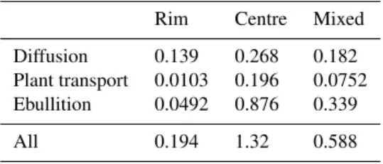
Figure 3.Modelled methane flux out of soil at(a)the rim,(b)the centre,(c)a mixed approach of 65 % rim plus 35 % centre, split into the different transport processes, and at(d)the rim, the centre and a mixed approach of 65 % rim plus 35 % centre combined, as a cumulative sum. Solid lines indicate 1 January; dashed lines indicate 1 April, 1 July and 1 October of the respective year. Please note the different scales. Table 1 gives the maximal values.
Table 1. Maximal values of the cumulative sums of modelled methane flux over the modelled time period for rim, centre and a mixed approach of 65 % rim plus 35 % centre for the different trans-port processes and combined in g C m−2, rounded to three non-zero digits.
Rim Centre Mixed
Diffusion 0.139 0.268 0.182 Plant transport 0.0103 0.196 0.0752 Ebullition 0.0492 0.876 0.339
All 0.194 1.32 0.588
3.2 Modelled methane flux in summer and winter The modelled methane fluxes at the rim and centre are differ-ent for the differdiffer-ent seasons (Fig. 2). While most of the mod-elled flux is positive (i.e. emission to the atmosphere), there are also uptake events. The spread of the flux is greater for the centre than for the rim in both summer and winter. While the majority of flux values in summer is positive at the cen-tre, it is more balanced at the rim. In winter, the methane flux is almost always zero, following the assumption that snow may hinder the exchange. However, at the centre, there are some rare events when uptake takes place. In the mixed ap-proach, which means 65 % rim and 35 % centre, the overall mean emission is about 0.0813 mg C m−2h−1 for the sum-mer period. The overall higher emissions at the centre are due to higher moisture and thus more favourable conditions for methane production in concert with lower methane oxi-dation rates.
3.3 Role of different transport processes
During most of the year, the diffusive methane flux is rather small at the rim (Fig. 3a) and sometimes slightly negative at the centre (Fig. 3b). The largest methane emissions, both at the rim and at the centre, occur during spring. In this season, the methane that is produced in the topsoil from late autumn on and accumulated during winter is released in the form of so-called spring bursts upon snow thaw.
emis-sions by ebullition and plant transport at the centre occur in this period (Fig. 3b).
In the mixed approach, only the diffusion of the rim alters the pattern of the emissions substantially (Fig. 3c). In total, the polygon centre accounts for a 6.8 times as large fraction of emissions as the rim due to the higher methane production under wetter conditions (Fig. 3d). This means a total share of 78.6 % of the methane emissions in the mixed approach is coming from the centre. Emissions at the rim are highest during spring, while they are highest at the centre during the mid and late season (Fig. 3d).
When comparing the total fluxes of the centre to the ones of the rim, diffusion is almost doubled, plant transport is 19 times as high, and ebullition is 18 times as high (Table 1). This results in almost 7 times higher total methane emissions at the centre than at the rim. At the rim, diffusion is more than 13 times as high as plant transport, while at the centre, it is just slightly higher than plant transport. Ebullition is about 4.5 times as high as plant transport both at the rim and at the centre. These differences are again due to the differences in soil moisture content, which allow more production un-der higher soil moisture and thus also lead to more methane emissions. On the other hand, plant transport is in principle a slower transport process than diffusion in water, but diffu-sion in water is much slower than diffudiffu-sion in air. Thus, un-der drier conditions, diffusion in air will transport the main portion of gas, but under wetter conditions, plant transport may increase relative to diffusion. With reduced soil air, the remaining velocity of the diffusion is almost of the same or-der of magnitude as the overall velocity of plant transport, in contrast to the velocity of diffusion mainly through air.
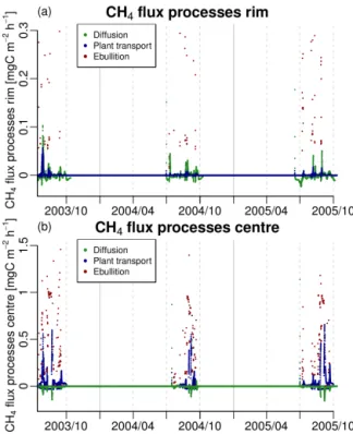
Splitting the total methane flux into several transport pro-cesses not only allows one to evaluate the relative contribu-tion of each process linked to rim or centre characteristics, but it is also possible to analyse differences in temporal pat-terns (Fig. 4a). As noted above, at the rim, the fluxes are much lower than at the centre (Fig. 4b), because less methane is produced under drier conditions, or methane becomes oxi-dised in the soil column. Ebullition makes up a large portion of the total budget at both microsites at isolated time steps, reflecting the nature of this process, while its total amount for the rim is rather small over longer time frames. At the rim, diffusion represents the second largest methane release but also substantial uptake during the season (Fig. 4a). The smallest flux portion at the rim is delivered by plant trans-port, which also shows some uptake. In contrast, at the cen-tre, plant transport plays a much more pronounced role, and diffusion fluxes are more negative. All these effects occur in the different hydrological regimes at the rim and at the cen-tre.
Furthermore, ebullition can only take place in soils with high soil moisture content, and this is more common at the centre than at the rim. Consequently, substantially more ebullition is found at the centre than at the rim. In the mixed approach, diffusion accounts for about 2.5 times of
Figure 4.Modelled methane flux out of the soil at the(a)rim and (b)centre, split into the different transport processes. Solid lines indicate 1 January; dashed lines indicate 1 April, 1 July and 1 Oc-tober of the respective year. Please note the different scales. Be-cause of the wide spread of high values, to as high as 39.3(a)and 86.6(b)mg C m−2h−1, a portion of 0.108 %(a)and 0.0609 %(b) values was cut to provide reasonable pictures. The minima of the values are−0.0234(a)and−0.158(b)mg C m−2h−1.
the emissions of plant transport, while ebullition accounts for 4.5 times of it. Overall, 0.588 g of carbon are emitted by each square metre during the modelled time period from 14 July 2003 to 11 October 2005.
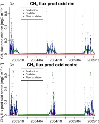
3.4 Production versus oxidation
Figure 5.Modelled methane amounts that get produced and oxi-dised at the(a)rim and(b)centre, split into the different processes. Solid lines indicate 1 January; dashed lines indicate 1 April, 1 July and 1 October of the respective year. Please note the different scales. The maxima of the values are 0.670(a)and 1.02(b)mgC m−2h−1.
Table 2. Change in the cumulative methane emissions over the modelled time period in %, when the parameter was modified by
±10 % compared to its default setting.
Parameter Lower range Upper range
fracCh4Anox −11.966 12.035 fracO2forOx+fracO2forPh −1.358 1.305
KmO2 −1.741 2.107
snowThresh 0.549 −0.090
resistRoot 0.024 0.195
thickExoderm 0.204 0.032
rootLength 0.024 0.195
rootDiam 0.024 0.195
tillerNumberMax 0.024 0.195 dominanceCarexAquatilis −0.151 0.344
3.5 Parameter sensitivity study
Results of the parameter sensitivity study are summarised in Table 2 and indicate that just one of the chosen param-eters, fracCH4Anox, has a major influence on the cumula-tive methane emissions when varied within a 10 % range. FracCh4Anox represents the fraction of methane produced under anoxic conditions compared to the total decomposition flux. For two more parameters, fracO2forOx+fracO2forPh and KmO2, the net effect was still larger than 1 %.
0.0
0.5
1.0
1.5
2.0
CH4 flux chamber2 summer
Rim Rim Centre Centre model 03−05 field 06 model 03−05 field 06
CH
4
flux chamber2 [mgC m
−
2 h
−
1]
Figure 6.Modelled methane flux out of soil at the rim and cen-tre compared to chamber measurements. Modelled values are only from the summer periods 2003 to 2005, which means less than 5 cm of snow are on the ground. Field measurements took place on 39 days from July to September 2006. Because of the wide spread of high modelled values, to as high as 86.8 mg C m−2h−1, a portion of 0.347 % modelled values was cut to provide a reasonable picture. The minimum of the modelled values is−0.0237 mg C m−2h−1.
FracO2forOx+fracO2forPh influences the available amount of oxygen for the methane oxidation, whereas KmO2 influ-ences the oxidation as the Michaelis–Menten constant for oxygen. For all remaining parameters, only negligible effects on the cumulative methane emissions were found.
3.6 Comparison to chamber measurements
Although the number of available field data is small and from a different year than the meteorological forcing data, the field measurements and model results are of the same order of magnitude (Fig. 6). Observations and model re-sults show higher centre values compared to the rim, but the model seems to underestimate occasional uptake events. For the rim, the model gives methane fluxes to the atmosphere of between−0.0237 and 39.3 mg C m−2h−1, with a mean of 0.0267 mg C m−2h−1, while the available field measure-ment values range from−0.111 to 0.881 mg C m−2h−1, with a mean of 0.154 mg C m−2h−1. For the centre, the model gives values between−0.0189 and 86.8 mg C m−2h−1, with a mean of 0.231 mg C m−2h−1, while the available field mea-surement values range from−0.0584 to 1.22 mg C m−2h−1, with a mean of 0.327 mg C m−2h−1. Besides higher mean values, the extremes are thus lower for the field measure-ments. This is due to the observation period excluding spring time, when the model calculates the highest emissions in the form of spring bursts.
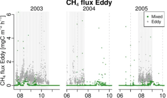
Figure 7.Modelled methane flux out of soil in a mixed approach of 65 % rim plus 35 % centre compared to eddy covariance mea-surements. Light grey background indicates measurement data cov-erage.Xaxes indicate the first day of the respective month of the year. Dashed lines indicate 1 July and 1 October of the respective year. Please note the cutouts in between the different years. Be-cause of the wide spread of high modelled values, to as high as 30.4 mg C m−2h−1, a portion of 0.0507 % modelled values was cut to provide a reasonable picture. The minimum of the modelled val-ues is−0.0235 mg C m−2h−1.
are highly variable in polygonal tundra environments and are of crucial importance for methane processes. Still, they may not be represented with the required detail by the model, so that the modelled conditions are the same as those at the mea-surement site. Thus, it is obvious that with coarser and dif-ferent hydrological conditions, the modelled methane fluxes per square metre for a 0.5◦grid cell cannot be identical to the point measurements of chambers. In particular, the low soil moisture in the hydrological conditions of the model may ex-plain the lower mean modelled methane fluxes compared to what is reported by chamber data.
3.7 Comparison to eddy measurements
Eddy covariance data had the best available data coverage of field measurements (light grey areas in Fig. 7). Overall model results are of the same order of magnitude as obser-vations, but there are also seasonal shifts between model results and measurements. This is due to a mismatch be-tween the real soil conditions at the measurement site and the modelled soil climate and hydrology that cannot be ex-pected to be the same as those in the field. The range of available measurements in the modelled period is 0.0233 to 4.59 mg C m−2h−1, with a mean of 0.609 mg C m−2h−1.
The range of modelled summer methane emissions in this time frame is−0.023 to 30.4 mg C m−2h−1, with a mean of 0.0813 mg C m−2h−1. If less than 5 cm of snow are on the ground, this is defined as summer time. Besides lower mean values, the model also shows higher extremes.
For this comparison, the same constraints hold like for the comparison to chamber data. The modelled fluxes differ from field measurements because of differences in thermal or
hydrological conditions. Critical are periods where observa-tions show substantial methane emissions while at the same time model results show only minor emissions, e.g. in au-tumn 2003 or spring 2004. During these periods, modelled soil temperature values below zero and snow cover result in modelled methane fluxes of virtually zero, while in reality soils might be warmer and gas diffusion through snow might be possible (see Sect. 4).
Still, Fig. 7 also shows some patterns that are present in both model results and observations, e.g. periods with in-creasing fluxes that are followed by a sudden decline in the fluxes in a cyclic manner during a single season. These pat-terns are linked to the changing soil moisture content. Unfor-tunately only the first season is covered well by field mea-surements, while the second misses the later part, and the third covers just a part within. The model shows the largest methane emissions during spring upon snow thaw for both rim and centre in the form of burst. There is still little ev-idence in field measurements of the occurrence and magni-tude of spring bursts, and to our knowledge no published data on this effect exist for Samoylov. In Sect. 4, we briefly re-view the evidence of spring bursts in other northern wetland areas to evaluate the representativeness of these events in the model results.
For additional results concerning modelled oxygen uptake, such as the mixed daily sum, seasonally split and cumulative sums, as well as transport process split, see Appendix B4.
4 Discussion
This paper aims to present the structure of a newly developed methane module for the JSBACH land surface scheme and evaluate its general performance against field observations. The new module itself is completely integrated into the larger framework of the JSBACH model; therefore, sensitivity tests can only be conducted using the full model and a clean sepa-ration between the existing structure and new components is not always possible. The interpretation and discussion of all findings should therefore consider that the functioning of the new methane module is to a large extent dependent on, and in many aspects limited by, the performance of the JSBACH model as a whole.
applied globally, certain limitations regarding the representa-tion of site-level observarepresenta-tions need to be taken into account. This situation is even aggravated due to the use of parameter settings from global fields, i.e. with a coarse spatial resolu-tion that aggregates condiresolu-tions over larger areas and thus nat-urally cannot provide the exact details for the field site where the reference fluxes were measured. Such systematic devia-tions in modelling framework and parameter configuradevia-tions will generate systematic differences between model output and site-level measurements. Accordingly, modelled hydro-logical conditions and amounts of decomposed carbon need to be considered when comparing modelled methane fluxes to the site-level observations and interpreting the spatiotem-poral differences.
As mentioned above, the JSBACH hydrology module has been designed for global applications and is not capable of capturing conditions in complex landscapes such as polygo-nal tundra. Therefore, for the Samoylov site, which we used for this site-level analysis, the modelled soil climate and hy-drology systematically deviate from those found in the field (Beer, 2016). We still chose to work at this site, because a highly valuable interdisciplinary dataset could be provided to evaluate different facets of the model output. To adapt the model to represent the complex hydrology, a mixed ap-proach of combining two different model runs was applied. This approximation implies a very simplified representation of the real hydrological conditions and cannot fully offset all site-level differences between model simulations and obser-vational datasets. Accordingly, systematic biases need to be considered when interpreting the findings. However, through this approach, we could demonstrate the paramount impor-tance of realistic hydrologic boundary conditions for simu-lations of the methane balance. In many aspects, details in the behaviour of the methane processes are tightly linked to the spatiotemporal variation of hydrological conditions; therefore, biases in hydrology are directly projected onto the methane processes.
Still, the authors believe that the comparison of methane simulations against selected site-level measurements is an important first step to evaluating the overall performance of the new module. It is obvious that the limitations of the observational database employed herein, i.e. using just one single observation site and focusing on the growing sea-son alone, cannot allow for a comprehensive assessment of the newly implemented algorithms. Accordingly, the lim-ited amount of available field measurements from chamber and eddy-covariance-based fluxes requires a careful inter-pretation when compared to model results, particularly re-garding the evaluation of JSBACH as a process-based global biosphere model. For the Arctic domain, methane emissions during shoulder and winter seasons have been shown to add considerably to the full annual budget, an aspect that we cannot evaluate based on the given database. Moreover, the question of temporal and spatial representativeness is com-plicated by the discontinuous nature of the methane fluxes
(e.g. Tokida et al., 2007a; Jackowicz-Korczy´nski et al., 2010; Tagesson et al., 2012). To overcome these limitations, in follow-up studies the authors plan to conduct model evalua-tions based on longer-term flux measurements, covering full annual cycles for multiple Arctic sites.
Even though eddy-covariance-based fluxes are regarded as the most reliable reference data source for longer-term site-level model evaluation, the influence of microsite variability in the area surrounding the tower clearly poses a challenge here. Particularly with respect to methane fluxes, pronounced variability in the distribution of soil organic matter and water content may lead to a mosaic of different source strengths. For the Samoylov domain, which is characterised by polygo-nal structures, the apparent differences between wet (centre) and moist (rim) areas were mimicked through the execution of two model runs with different settings. Still, the footprint composition of the eddy covariance tower might not match the mixed approach of 65 % rim and 35 % centre used for modelling (Sachs et al., 2010). Even though this mixture gen-erally captures the composition of the larger area surround-ing the tower, particularly when footprints are smaller dursurround-ing daytime, the reduced field of view of the sensors might focus on areas that are wetter or drier than the average. The concept of combining two separate model runs has to be regarded as an approximation to cope with the hydrological constraints of a global model on the one hand and the complex landscape on the other.
The model application for remote permafrost areas may also be limited by the availability of long-term and com-plete observations of meteorological data to be used as model forcing. Forcing data and methane fluxes are required for the same time period, which optimally lasts over 1 or more years. When going towards regional to global applications, this new model might be additionally compared to regional or global atmospheric inversion results (e.g. Bousquet et al., 2011; Berchet et al., 2015) or data-driven upscaling of eddy-covariance- or chamber-based observations (e.g. Christensen et al., 1995; Marushchak et al., 2016).
Within the methane module presented in this work, the discretisation as well as the pore volume are variable. This requires that the time step of calculation and the diffusion coefficients must fit to the thicknesses of the soil layers. If not set up properly, instabilities like oscillations or unrealis-tic behaviour like negative concentrations may occur. How-ever, because the new methane module has been designed to be flexible in this respect, adjustments can easily be made in case numerical problems arise.
A parameter sensitivity study (Sect. 3.5) shows that the uncertainty of the resulting methane emissions scales lin-early only for one parameter with the uncertainty of that pa-rameter. This parameter represents the amount of methane produced under anoxic conditions compared to the total de-composition flux of carbon dioxide and methane combined
[CH4]
[CO2]+[CH4]
methano-genesis chemical reaction equation and based on laboratory and field data (Segers, 1998), this parameter was chosen to be 0.5 in Eq. (2). In other models, this parameter is used as an effective parameter and has been tuned to match ultimate methane and carbon dioxide emissions from soil to the atmo-sphere in the absence of an explicit representation of oxygen and hence methanotrophy (Wania et al., 2010).
Regarding the assumptions concerning fluxes during win-ter time or plant transport, according to recent findings (Zona et al., 2016; Marushchak et al., 2016), the settings chosen within the context of this work might be oversimplifying the actual processes in the field. The implemented mecha-nism that prevents gas exchange with the atmosphere once the snow cover reaches a depth of 5 cm is a very crude ap-proximation of the snow cover influence. It resulted from bi-ases in the modelled hydrological conditions in winter, where freezing of relatively dry soils led to oxic soil conditions that facilitated methane transport into the soil. The next iteration of the model development will include a more sophisticated, process-based representation of methane diffusion through snow. This upgrade, however, needs to be coupled to a major restructuring of several model components and thus cannot be reconciled with the model version presented within the context of this study.
The implementation of the plant transport follows a mech-anistic approach, but its definition is limited by the avail-ability of observational evidence on e.g. diffusion velocities. Therefore, the parameter settings used in this study are sub-ject to high uncertainty. The value for the diffusion coeffi-cient in the exodermis was chosen to be 80 % of the diffusion coefficient in water (C. Knoblauch, personal communication, 2014). The subsequent gas transport within the aerenchyma is assumed to be as quick as diffusion in air. With this set-up, the effective barrier of the root exodermis will limit the plant transport efficiency and therefore act as a dominant control for this emission pathway. The thickness of this bar-rier has a large influence on plant transport as well; i.e. a thinner root exodermis would lead to increased plant trans-port. While this parameter is relatively easy to define, the cumulative surface area of all gas transporting roots in the soil column is difficult to constrain. Considering our basic assumption that plant transport is slower than diffusion in water, the general patterns of flux processes and soil moisture for rim and centre conditions appear plausible. Regarding the quantitative flux rates, however, the fraction of the total flux emitted through plant transport in the model tends to be too low. With larger root surface leading to increased plant trans-port, we therefore could use this setting as a tuning param-eter to improve this issue. However, the oxygen available to consume methane also plays another modulating role, par-ticularly for plant transport. Accordingly, new observational evidence would certainly improve the associated uncertain-ties; therefore, this issue is subject to ongoing investigations. With the new methane module, designed to be flexible
re-garding these kinds of settings, parameter adjustments with respect to newer findings can easily be implemented.
The contribution of labile root exudates to methane pro-duction and emission has been largely neglected in exist-ing model implementations and is also not considered in this model configuration. This is also an understudied process in field experiments and can only be estimated indirectly. The rate of root exudates is linked to the nutrient availability in soils, with more root exudates present in plants located in nutrient-poor wetland soils (Koelbener et al., 2010). The wet-land soils in Arctic tundra are known to be nitrogen-limited (Melle et al., 2015; Gurevitch et al., 2006). The plant growth in the polygonal lowland tundra of Indigirka, Russia, is co-limited by nitrogen and phosphorus, and only about 5 % of the total nitrogen soil content is active in the biological frac-tion (Beerman et al., 2015). The presence of vascular plants in Arctic wetlands supports the production of highly labile low molecular weight carbon compounds which can promote methane emissions through their methanogenic decomposi-tion (Ström et al., 2012). Indirect evidence of the role of root exudates in methane production in polygonal ponds and water-saturated soils in Samoylov is presented by Knoblauch et al. (2015). The authors found almost 4-fold higher poten-tial methane production rates in vegetated sites compared to the non-vegetated ones, both with the same C and N soil concentrations. Thus, the contribution to methane emissions from wetland soils in Arctic tundra due to the decomposi-tion of root exudates should be taken into account in models. This will allow the understanding of the role of root exudates under present climate conditions. On the other hand, the po-tential nutrient mobilisation in soils due to permafrost degra-dation under climate change (Kuhry et al., 2010) may reduce the role of root exudates in methane emissions. However, the current JSBACH configuration lacks a full soil nutrient cycle, and the assimilation of nutrients by plant roots, as well as the contribution of root exudates to the total methane emissions, cannot be modelled at this point.
In Samoylov, the minimum of modelled daily sums of methane emissions during summer is smaller and the max-imum much higher for rim and centre compared to measure-ments published by Kutzbach et al. (2004). However, these observations do not include spring bursts with very short but also very high emissions or even dry phases with small up-take. On the other hand, the mean of those measurements is 3 times as high for the rim and 3.5 times as high for the centre compared to the modelled daily sums in summer (Ta-ble 3). But such high modelled emissions are rather rare, and the general level of modelled values is lower than in obser-vations (Fig. 7).
Table 3.Modelled daily methane flux for the summer periods 2003 to 2005 for the rim, centre and a mixed approach of 65 % rim plus 35 % centre in mg CH4m−2d−1, rounded to three non-zero digits.
Summer means less than 5 cm of snow are on the ground. Please note the different unit here.
Min Mean Max
Rim −0.690 1.34 208 Centre −0.208 8.21 385 Mixed −0.521 2.90 135
Table 4. Modelled hourly methane flux for the summer periods 2003 to 2005 for the rim, centre and a mixed approach of 65 % rim plus 35 % centre in mg C m−2h−1, rounded to three non-zero digits. Summer means less than 5 cm of snow are on the ground.
Min Mean Max
Rim −0.0237 0.0267 39.3 Centre −0.0189 0.231 86.8 Mixed −0.0235 0.0813 30.4
Delta region is much colder and drier compared to these sites, suggesting that lower flux rates are indeed reasonable. Furthermore, the Samoylov site is characterised by mineral soils containing substantially lower organic carbon as a sub-strate for methane production than the organic soils at the BOREAS site and the mire in Abisko. Compared to mea-surements done by Desyatkin et al. (2009) on a thermokarst terrain at the Lena River near Yakutsk, our mean results are well within the measurement range when comparing our rim to the drier sites, our centre to the wetter sites, and our mixed approach to the entire ecosystem (Table 4). However, cli-mate and environmental conditions in this study were very different from those observed in Samoylov; thus, this com-parison can only be regarded as a rough guideline. Nakano et al. (2000) measured methane fluxes at Tiksi near the mouth of the Lena River. While our mean value at the rim is 4.5 times as high as the mean measurements in Tiksi, the mean at the centre is 5.5 times as high as our mean value (Table 3). The modelled minimum is lower for the centre but compara-ble for the rim.
The large methane spring burst simulated by the model at both the rim and centre may represent the release of methane that has been accumulated during winter in the topsoil below the snow layer. To our knowledge, there is no observational reference of spring bursts measured in Samoylov. However, evidence of these events have been presented for other wet-land areas using chambers and eddy covariance measure-ments, e.g. in northern Sweden (Jammet et al., 2015; Fri-borg et al., 1997), in Finland (Hargreaves et al., 2001), in northern Japan (Tokida et al., 2007b) and in Northeast China (Song et al., 2012). These studies suggest the presence of spring thaw emissions of methane that occur sporadically
over short periods in the form of bursts. The magnitude of the spring bursts can exceed the mean summer fluxes by a factor of 2 to 3. Although spring emissions can account for a large share of the total annual fluxes, their occurrence, du-ration and magnitude are still uncertain. To adequately char-acterise the spring bursts in Samoylov, it is necessary to per-form dedicated field measurements during the spring thaw period. These results will then help to evaluate the represen-tativeness of the modelled spring bursts. In future model it-erations, the spring bursts will also be evaluated for larger spatial scales.
In Zona et al. (2009), several measurements of methane emissions in the Arctic tundra are presented. Despite our mean values being located towards the lower end, our min-imum, mean and maximum values fit well within the given range. Bartlett et al. (1992) measured methane fluxes near Bethel in the Yukon–Kuskokwim Delta, Alaska. The pro-vided values for upland tundra compare well to our mean and minimum values. However, the model maximum fluxes are higher than the measurement values for upland tundra, but still well within the range of measured values for wet meadow, which has higher moisture contents than upland tundra. In fact, the highest values are calculated if soil mois-ture is highest, so despite being more on the lower end of this waterlogged landscape type’s emissions, they also fit well therein. In summary, the variability of results of this pan-Arctic survey indicates that methane budgets within all these places are influenced by different conditions in terms of weather, hydrology and carbon pools. Accordingly, the good agreement of our modelled values with these references confirms that our results are within a plausible range at the greater picture, but a detailed evaluation cannot be performed without in-depth analysis of the site-level conditions.
scheme of the current model version, it would be desirable to use other approaches like TOPMODEL (e.g. Kleinen et al., 2012) that would allow one to represent the fraction of the inundated area in a model grid cell based on the topography profile. This would provide a modelled wetland extent and a representation of the water table depth in saturated soils, especially for large-scale applications. This step has been considered and will be included in future model iterations. Despite being a complex process model, the interplay of the processes is consistent. Thus, the influence of climate and hy-drology on methane fluxes can be studied in detail. Knowing the dominating processes and environmental conditions pro-vides useful information about the complex behaviour of the methane dynamics in permafrost soils. To summarise, a lot of information can be gained from using this model that may all help understand the complex network of drivers, influenc-ing factors and constraints that govern the methane balance in periglacial landscapes.
5 Conclusions
The aim of this study was to develop a more detailed and consistent process-based methane module for a land sur-face scheme which is also reliable in permafrost ecosystems. Based on previous work by Wania et al. (2010) and Walter and Heimann (2000), the JSBACH land surface scheme of the MPI-ESM global Earth system model has been enhanced for this purpose. The new methane module of JSBACH-methane represents JSBACH-methane production, oxidation and trans-port. Methane transport has been represented via ebullition, diffusion and plant transport. Oxygen can be transported via diffusion through soil pores and plant tissue (aerenchyma). Two methane oxidation pathways are explicitly described: one takes the amount of soil oxygen into account and the other explicitly uses oxygen that is available via roots (rhi-zospheric oxidation). All methane-related processes respond
to different environmental conditions in their specific ways. They increase or decrease according to their requirements with changing soil moisture, temperature or ice content. The differences between the processes, seasonal differences as well as differences between the rim and centre microsites have been shown.
When combined with a module for water-saturated soil conditions like TOPMODEL (e.g. Kleinen et al., 2012), such a methane-advanced land surface scheme can be used to esti-mate the global methane land fluxes, including for periglacial landscapes. These regions are rich in soil carbon (Hugelius et al., 2014) and show good conditions for methane production (Schneider et al., 2009). However, they are often remote and rather hard to investigate. Thus, process-based modelling can contribute to understanding the role of methane emissions as long as widespread and long-term measurements remain scarce. In addition, the role of methane for future permafrost carbon feedbacks to climate change can be studied. For these reasons, the module in this study is also highly integrated with permafrost and wetland processes, e.g. changing pore space in the soil because of freezing and thawing or chang-ing water table depths due to changchang-ing soil water content. In a first comparison with site-level field measurements, suffi-ciently good agreements could be shown, despite the module not having been adjusted to site-specific processes or fea-tures. Coupling such a land surface scheme to atmosphere and ocean schemes in an Earth system model will provide the basis for studying methane-related feedback mechanisms to climate change.
6 Code availability