www.atmos-meas-tech.net/6/2521/2013/ doi:10.5194/amt-6-2521-2013
© Author(s) 2013. CC Attribution 3.0 License.
Atmospheric
Measurement
Techniques
Retrieval of nitric oxide in the mesosphere and lower thermosphere
from SCIAMACHY limb spectra
S. Bender1, M. Sinnhuber1, J. P. Burrows2, M. Langowski2, B. Funke3, and M. López-Puertas3 1Karlsruhe Institute of Technology, Karlsruhe, Germany
2University of Bremen, Bremen, Germany
3Instituto de Astrofísica de Andalucía, CSIC, Granada, Spain
Correspondence to:S. Bender ([email protected])
Received: 28 March 2013 – Published in Atmos. Meas. Tech. Discuss.: 12 April 2013 Revised: 20 August 2013 – Accepted: 20 August 2013 – Published: 27 September 2013
Abstract.We use the ultra-violet (UV) spectra in the range 230–300 nm from the SCanning Imaging Absorption spec-troMeter for Atmospheric CHartographY (SCIAMACHY) to retrieve the nitric oxide (NO) number densities from atmo-spheric emissions in the gamma-bands in the mesosphere and lower thermosphere. Using 3-D ray tracing, a 2-D retrieval grid, and regularisation with respect to altitude and latitude, we retrieve a whole semi-orbit simultaneously for the altitude range from 60 to 160 km.
We present details of the retrieval algorithm, first re-sults, and initial comparisons to data from the Michelson Interferometer for Passive Atmospheric Sounding (MIPAS). Our results agree on average well with MIPAS data and are in line with previously published measurements from other instruments. For the time of available measurements in 2008–2011, we achieve a vertical resolution of 5–10 km in the altitude range 70–140 km and a horizontal resolution of about 9◦ from 60◦S–60◦N. With this we have indepen-dent measurements of the NO densities in the mesosphere and lower thermosphere with approximately global coverage. This data can be further used to validate climate models or as input for them.
1 Introduction
Observations of a number of Antarctic and Arctic winters have shown that in polar regions, downwelling of nitric ox-ides (NOx = N, NO, NO2) from the upper mesosphere and
lower thermosphere can provide a significant source of NOx
in the polar upper and middle stratosphere, see, for
exam-ple, Siskind et al. (2000), Funke et al. (2005a), and Randall et al. (2009). However, it is not clear whether the source of these NOx intrusions is from auroral production in the
lower thermosphere, or due to local production in the meso-sphere by relativistic electrons, see, e.g. Callis et al. (1998) and Sinnhuber et al. (2011, 2012). The measurements with the SCanning Imaging Absorption spectroMeter for Atmo-spheric CHartographY (SCIAMACHY) on the European re-search satellite Envisat quantify this important coupling be-tween the sun and the upper atmosphere as they are the only measurements with a good sensitivity, temporal resolution, and global coverage in the middle and upper mesosphere (70–90 km).
measurements of the upwelling radiation at the top of the atmosphere on the sunlit side of the orbit. In phases A (feasi-bility study) and B (definition study), SCIAMACHY was de-scoped to one instrument making solar lunar occultation and alternate limb and nadir measurements (Burrows et al., 1995; Bovensmann et al., 1999). As a result of data rate limitations on Envisat, the limb scanning mode of SCIAMACHY was restricted from−2 km to about 93 km. However, in order to probe the mesosphere and thermosphere, the mesosphere and lower thermosphere (MLT) measurements mode was adopted as an additional limb mode since 2008. This manuscript ad-dresses studies using this measurements mode.
We use a part of SCIAMACHY’s UV channel 1 (214– 334 nm) to infer the NO number densities from atmospheric emissions of the gamma bands in the mesosphere and lower thermosphere. The gamma bands were already used in the retrieval of NO from rocket and satellite experiments. The rocket experiments (Cleary, 1986; Eparvier and Barth, 1992) have a very limited spatio-temporal coverage as they are re-stricted to single-day flights, in August 1982 (Cleary, 1986) and in March 1989 (Eparvier and Barth, 1992) and to the area close to the starting location, Poker Flat, Alaska, in both cases.
Satellite measurements of nitric oxide (NO) were first done with the SBUV spectrometer on board the Nimbus 7 satellite by Frederick and Serafino (1985) in nadir geometry using the NO (1,4) gamma emission at 255 nm. Further pre-vious satellite experiments using the NO gamma bands in the ultra-violet spectral range include the Student Nitric Oxide Explorer (SNOE, Barth et al., 2003) which measured nitric oxide in the thermosphere (97 to 150 km) from March 1998 until December 2003. Results are published until Septem-ber 2000 and are used by the NOEM empirical model of ni-tric oxide in the MLT region (Marsh et al., 2004). The Iono-spheric Spectroscopy and AtmoIono-spheric Chemistry (ISAAC, Minschwaner et al., 2004) satellite performed measurements at 80–200 km and results are published for November 1999– December 1999.
Measurements of NO in the mesosphere using microwaves were done by the Sub-Millimitre Radiometer (SMR) on board the Odin satellite. Infrared measurements were per-formed by the Optical Spectrograph and InfraRed Imaging System (OSIRIS) on board the Odin satellite which mea-sured nighttime NO from NO2 airglow emissions up to
100 km (Sheese et al., 2011). Further infrared instruments are the Atmospheric Chemistry Experiment Fourier trans-form spectrometer (ACE-FTS) (Kerzenmacher et al., 2008) and the Michelson Interferometer for Passive Atmospheric Sounding (MIPAS) also on the Envisat satellite. The MI-PAS instrument measures the vibrational–rotational emission lines of NO with its infrared spectrometer directly (Funke et al., 2005b; Bermejo-Pantaleón et al., 2011). It shares the satellite with SCIAMACHY but is oriented to view in the opposite direction. This means that MIPAS samples the air at approximately the same tangent points but with a delay of
about 50 min. With its special upper atmosphere (UA) mode which, however, is also not continuous, it provides another independent verification of our results.
This paper is organised as follows: we present some details about SCIAMACHY and its MLT mode in Sect. 2, Sect. 3 goes into detail about the NO gamma bands and the retrieval method. Finally, our results and the comparisons to MIPAS data and the NOEM model are shown in Sect. 4.
2 SCIAMACHY MLT mode
SCIAMACHY is a limb sounding experiment aboard the Eu-ropean Envisat satellite flying in a sun-synchronous orbit at approximately 800 km altitude since 2002 (Burrows et al., 1995; Bovensmann et al., 1999). The wavelength range of SCIAMACHY extends from UV to the near infrared (220– 2380 nm). From July 2008 to April 2012, SCIAMACHY performed observations in the mesosphere and lower ther-mosphere (MLT, 50–150 km) regularly twice per month; this limb mesosphere-thermosphere state was coordinated with the MIPAS upper atmosphere (UA) mode once every 30 days.
The MLT mode sampled the mesosphere and lower ther-mosphere at 30 limb points from 50 to 150 km with a vertical spacing of about 3 km. The scans were scheduled in place of the usual nominal mode limb scans from 0 to 90 km, so that the rest of the measurements within the orbit sequence remained unchanged and there were around 20 limb scans along a semi-orbit. This compares well with the MIPAS mea-surement sequence, which collects limb scans every four to five degrees and its UA mode scans from 50 to 170 km.
The use of the NO gamma bands for the SCIAMACHY retrieval, where the first electronic state needs to be excited, restricts the useful measurements to times with available sun-light for this excitation. That means we can only retrieve the NO densities at daytime with SCIAMACHY. In contrast to that, the use of the infrared bands by MIPAS allows them to measure the NO densities at night-time as well. We take this into account when comparing the measured densities from both instruments.
3 Retrieval algorithm
Table 1.NO emissivity parameters used in the paper for the three NO gamma bands used for the retrieval.
(0, 2) (1, 4) (1, 5)
λv′0[nm] 226.5 215.1 215.1
λv′v′′[nm] 247.4 255.4 267.4
fv′0[10−4] 3.559 7.010 7.010
ωv′v′′ 0.2341 0.1115 0.0971
NOEM model (Marsh et al., 2004) as the a priori data for the retrieval.
3.1 NO gamma bands
The NO gamma bands result from the electronic transition of the NO molecule from the first excited state,A26+, to the ground stateX25. The excitation happens by absorbing solar UV light, which restricts our retrieval to daytime nitric oxide, as discussed at the end of Sect. 2.
The various gamma bands have different advantages and disadvantages for retrieval. The ones to the vibrational ground state of the electronic ground state, e.g. the (1, 0), (2, 0) transitions, have the advantage of high emission rates and the disadvantage of self-absorption, see, for ex-ample, Eparvier and Barth (1992) and Stevens (1995). This makes the atmosphere optically thick with respect to these bands and the emissivity depends on the total slant column density along the line-of-sight (Eparvier and Barth, 1992). In contrast to that, transitions to a different vibrational state, e.g. the (0, 1), (0, 2), or (1, 4) transitions, have a lower emissivity, but the probability of self-absorption is greatly reduced. 3.2 NO emissivity calculation
The emissivities of the NO gamma bands are calculated following Stevens and others (Eparvier and Barth, 1992; Stevens, 1995). The emission rate factorsgv′v′′for the
transi-tion from the vibratransi-tional statev′of the electronically excited
state to the vibrational statev′′of the electronic ground state
are given by the sums over all rotational emission factors
gj′j′′ (see Eparvier and Barth, 1992 and references therein
and Stevens et al., 1997), which are given by
gj′j′′=
S(j′j′′)
2j′+1ωv′v′′
·
∞
X
j=|3+6|
π e2 mc2λ
2
j′jπ Fj′jfv′0
S(j′j )
2j+1
Nj
N0
. (1) Here,Sare the Hönl–London factors for the rotational tran-sitions (Earls, 1935; Schadee, 1964; Tatum, 1967),ωis the branching fraction,λ the transition wavelength, π F is the solar irradiance at that wavelength taken from Chance and Kurucz (2010), and f is the oscillator strength. Nj is the
NO population of the rotational level j and N0 the
popu-lation of the zero vibrational level of the electronic ground
240 245 250 255 260 265 270 275 280
wavelength [nm]
0.0
0.5
1.0
1.5
2.0
2.5
3.0
em
issi
vit
y [
10
-7
ph
/m
ole
c/s]
NO emissivity at 200 K
0-2
1-4
0-3
1-5
0-4
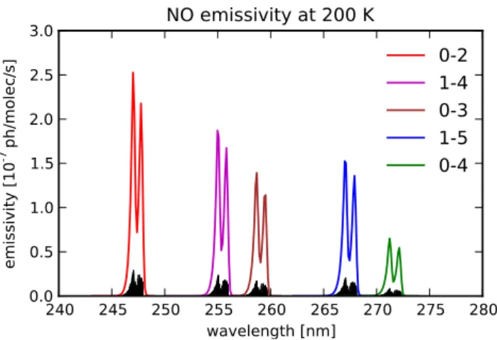
Fig. 1.NO emissivities calculated for a temperature of 200 K for a selected number of gamma bands. The small black lines indicate the individual rotational emission lines within the vibrational transi-tion bands and the coloured lines are the emissivity bands resulting from binning to the SCIAMACHY spectral resolution and convolv-ing with the respective spectral slit function.
state (Eparvier and Barth, 1992). The most important param-eters for the emissivity calculation are summarised in Ta-ble 1, listing the selected values from Luque and Crosley (1999). The molecular constants can be found in Table 2 of Eparvier and Barth (1992).
The calculated spectrum at 200 K for a selected number of gamma bands is shown in Fig. 1, where the small black lines indicate the individual rotational transitions and the larger envelope lines result from binning to the SCIAMACHY res-olution and the convres-olution with the spectral slit function of the instrument. The spectra are calculated using spec-troscopic data (oscillator strengths and branching fractions) from Luque and Crosley (1999).
The gamma bands shown in Fig. 1 are the ones that are visible in SCIAMACHY’s UV channel 1. For the retrieval we use the three gamma bands with the largest emissivities in that spectral range, which are the (0,2), the (1,4), and the (1,5) bands at 247, 255, and 267 nm, respectively. These are all non-resonant bands and the line-of-sight should be opti-cally thin. Additionally including the (0,3) band gives a neg-ligible improvement of the results but increases the memory needs and processing time because of the larger matrices in-volved in the retrieval.
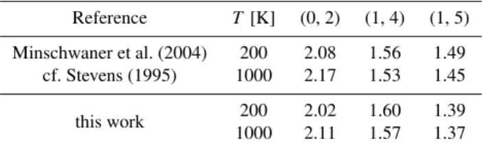
Table 2.NO band integrated emission rate factors (in 10−6ph s−1) at 200 and 1000 K for theγbands used in the retrieval. Top row: re-sults from Stevens (1995), using the parameters from Piper and Cowles (1986), and used for NO retrieval by Minschwaner et al. (2004). Bottom row: factors used in this work, using the parameters from Luque and Crosley (1999).
Reference T [K] (0, 2) (1, 4) (1, 5)
Minschwaner et al. (2004) 200 2.08 1.56 1.49 cf. Stevens (1995) 1000 2.17 1.53 1.45
this work 200 2.02 1.60 1.39 1000 2.11 1.57 1.37
The variation of the emissivity over the temperature range from 200 to 1000 K is smaller than five percent, see Ta-ble 2. The temperature range found in the thermosphere is smaller (200 K. . . 600 K) such that the error introduced by using model temperatures from NRLMSISE-00 (Picone et al., 2002) instead of temperatures measured by MI-PAS (Bermejo-Pantaleón et al., 2011) is small, although de-viations around thirty up to sixty percent from the model were found.
3.3 Radiative transfer
The general forward model is the functional relation
y=F (x) (2)
between the measurementsyand the quantities of interestx. In the case discussed in this paper, the measurements are the spectral irradiances at the frequencyν (or at wavelengthλ) at the satellite point,Iν. Of interest are the number densities
of NO at the retrieval points,x(s).
The measured irradianceIν at the frequencyνis given by
the radiative transfer equation as the integral over the line-of-sight:
Iν=
Z
LOS
(x(s)γν(s)Fν′(s)+σR̺air)e−τνds (3)
≈γ Fe−τ Z
LOS
x(s)ds=γ Fe−τ·̺sc, (4)
In Eq. (3),xis the number density of the species,γthe emis-sivity factor, andF the solar irradiance at the excitation fre-quencyν′. The Rayleigh part of the spectrum,σ
R̺air, is fitted
as a spectral background signal.
Since we use non-resonant transitions, the line-of-sight is optically thin with respect to self-absorption (Stevens et al., 1997). Retrieving number densities above 60 km has the ad-ditional advantage that quenching is negligible and the op-tical depth is mainly determined by the ozone and air ab-sorption along the line-of-sight and along the line from the
sun (Stevens et al., 1997). This absorption is independent of the NO number densityxand modifies the column emission rate as seen by the instrument by the constant factor e−τ. The
optical depthτ is given by
τ=X
i
Z
LOS
σiabs̺iabsds , (5)
where the sum includes all absorbing species along the line-of-sight. This leaves us with the linear relationship of the in-tensity to the slant column density̺scin Eq. (4).
3.4 Retrieval algorithm
The general problem is to invert Eq. (2) to extractxfromy, where there are usually a different number of measurements (y) than unknowns (x), which means that Eq. (2) is under-determined or overunder-determined. In the case of an overdeter-mined system, this inversion problem can be solved by min-imising
kKx−yk2, (6)
whereKis the Jacobian of the forward model Eq. (2). The measurementsy are the slant column densities from fitting the calculated NO spectra to the measured ones. We fit each NO gamma band individually to get three separate measure-ments (and errors) of the slant column density at the tan-gent points. The measurement vector y has the dimension 3×(number of tangent points) and the results from all three gamma bands are used simultaneously to retrieve the number densityx.
In the case of an underdetermined system, additional con-straints are needed. These are given by the a priori input, i.e. approximate knowledge of the solutionx. The minimisation problem then changes to
kKx−yk2
S−y1
+ kx−xak2S−1 a
, (7)
whereSare the covariance matrices and the subscript “a” in-dicates the a priori quantities. Doing a 2-D-retrieval, we ad-ditionally constrain the solutions to not vary too much with altitude and latitude by introducing regularisation matrices Ralt and Rlat, see Scharringhausen et al. (2008a) and
Lan-gowski et al. (2013). This then leads to the minimisation of kKx−yk2
S−y1
+ kx−xak2S−1 a
+λaltkRalt(x−xa)k2+λlatkRlat(x−xa)k2(8)
in our case. The a priori covariance matrixSais chosen asλaI
with an empirically tuned parameterλa. The regularisation
matricesRalt andRlat are discrete first derivative matrices
with respect to altitude and latitude. Their effect is a smooth-ing of the solution in these directions, preventsmooth-ing large oscil-lations by carefully choosingλaltandλlat. The regularisation
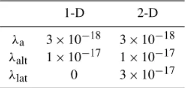
Table 3.Regularisation parameters as used in the NO retrieval from SCIAMACHY limb scans.
1-D 2-D
λa 3×10⁻¹⁸ 3×10⁻¹⁸
λalt 1×10⁻¹⁷ 1×10⁻¹⁷
λlat 0 3×10⁻¹⁷
The solution of Eq. (8) is obtained by an iterative algo-rithm. Defining a combined regularisation matrixRas R:=S−a1+λaltRTaltRalt+λlatRTlatRlat, (9)
the intermediate solution is given by (von Clarmann et al., 2003; Funke et al., 2005b)
xi+1=xi+
KTS−y1K+R−1
·hKTS−y1(y−yi(xi))+R(xa−xi)
i
.(10) 3.5 Model input
Our retrieval uses model input to provide an initial guess for the number density and to improve the convergence of the iteration. The a priori input stems from the NOEM model (Marsh et al., 2004), which is also used by the MI-PAS NO retrievals (Funke et al., 2005b). It is an empiri-cal model based on SNOE observations (Barth et al., 2003) and constructed for the altitude range from 100 to 150 km only (Marsh et al., 2004). The extension downwards and up-wards is done by using constant number densities indepen-dent of altitude. Hence, the use of the NOEM model for alti-tudes below 100 km is questionable, but we use it because of our direct comparisons to MIPAS data.
Another input necessary for the emissivity calculation of the NO rotational transitions are the atmospheric tem-peratures. These are calculated using the NRLMSISE-00 model (Picone et al., 2002) which has as main input parame-ters the geomagneticApindex and the solar radio fluxf10.7.
These data were taken from the Space Physics Interactive Data Resource (SPIDR) service (NGDC and NOAA, 2011) of the National Geophysical Data Center (NGDC) of the Na-tional Oceanic and Atmospheric Administration (NOAA).
4 Results
4.1 NO number density
To illustrate the results of our retrieval, we choose one exam-ple orbit, 41 467 from 3 February 2010, to show the individ-ual steps. For one selected tangent point, 71◦N, 105 km, the spectral fit for the NO (0,2) transition is shown in Fig. 2. This latitude and altitude were chosen such that the NO content in that region is supposed to be non-negligible as indicated by
245
246
247
248
249
wavelength [nm]
6
4
2
0
2
4
6
8
resi
du
al
rad
ian
ce
[p
h/c
m
2
/s/n
m]
1e9
scd: 3.121e+16 cm
-2error: 9.555e+15 cm
-2Orbit 41467, 02, Lat: 70.8 deg, Lon: 182 deg, Alt: 106 km.
Fig. 2.NO (0,2) spectral fit, showing the residual spectra (red) after dark-current subtraction and Rayleigh background fit, and the fitted NO spectrum (blue) with a low order polynomial as a baseline.
80 60 40 20 0 20 40 60 80
latitude [deg]
60
80
100
120
140
altitude [km]
2010-02-03 Orbit 41467, NO 02
-2
-1
0
1
2
3
4
5
6
sla
nt
co
lum
n d
en
sit
y [
10
16
/cm
2
]
Fig. 3.NO slant column densities for the (0,2) transition along the sample orbit (no. 41467, 3 February 2010).
previous measurements from SNOE (Barth et al., 2003). As the figure shows, the UV spectra can be noisy, i.e. the NO signal is near the noise threshold, introducing errors into the fitted slant column densities and reducing the signal-to-noise ratio (SNR). These errors are taken into account by the re-trieval algorithm as the covariance matrix Sy, see Eqs. (7)
and (8), giving less weight to points with a low SNR. The resulting slant column densities for the same orbit are shown in Fig. 3 for the (0,2) transition. The largest slant column densities for all three lines (the other two are not shown here) are observed at approximately the same tan-gent points, namely in the region from 60◦N–70◦N and at
altitudes around 100 km.
The zonal mean (60◦N–90◦N) for the line-of-sight
-2 -1 0 1 2 3 4 5 6 7 LOS emissivity [109photons/s/cm2]
40 60 80 100 120 140 160
altitude [km]
LOS emissivity 60N--90N
-5 0 5 10 15 20 25 30 35 40 slant column density [1015/cm2]
slant column density 60N--90N
-0.5 0.0 0.5 1.0 1.5 2.0 2.5 NO number density [108/cm3]
NO number density, 60N--90N NOEM apriori null apriori
Fig. 4.Zonal mean (60◦N–90◦N) integrated NO emissivity profile (3 February 2010) (left panel), zonal mean fitted slant column densities (middle panel), and zonal mean NO number densities (right panel) using the NOEM model as a priori input (blue line) and without prior assumptions (red line). The error bars show the 3σ confidence interval.
80 60 40 20 0 20 40 60 80
latitude [deg]
60
80
100
120
140
160
altitude [km]
2010-02-03 Orbit 41467, NO 02+14+15
0
1
2
3
4
nu
mb
er
de
nsi
ty
[10
8
/cm
3
]
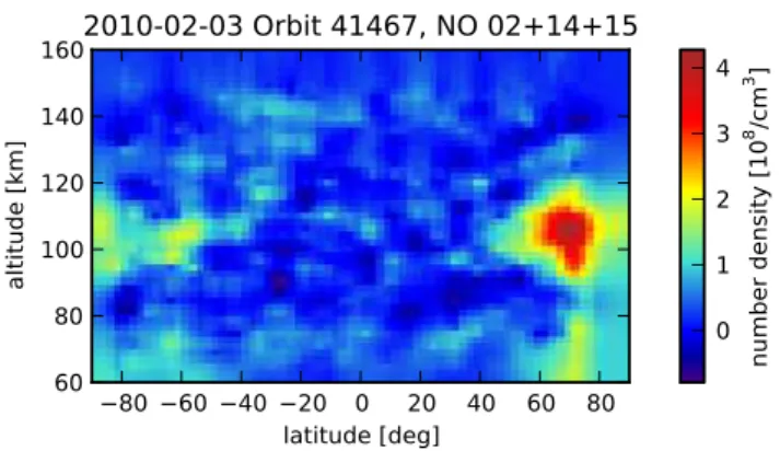
Fig. 5. Retrieved NO number densities along the sample orbit (no. 41467, 3 February 2010).
in the right panel of Fig. 4. It shows that the altitude of the largest number density is above the peak emissivity and peak slant column density. This is the result of the retrieval algo-rithm that takes into account that the slant column density is given by the total NO emission along the line-of-sight which is largest at a tangent point where the line-of-sight includes the whole NO layer in the thermosphere, i.e. slightly below 100 km.
Using the retrieval algorithm as described in Sect. 3, the calculated number density distribution along the orbit is shown in Fig. 5. As already indicated by the slant column densities and the number density profile in Fig. 4, the max-imum here is between 60◦N and 70◦N and at an altitude of around 100–110 km. In the northern winter there is polar night at latitudes north of 80◦, hence the retrieval of NO in this region is not possible.
0.1 0.0
0.1
0.2
0.3
AKM
60
80
100
120
140
160
altitude [km]
20100203: Orbit 41467, NO 02+14+15
AKM (alt) 71
Fig. 6.Altitude averaging kernel matrix elements for a sample orbit (no. 41467, 3 February 2010).
4.2 Resolution
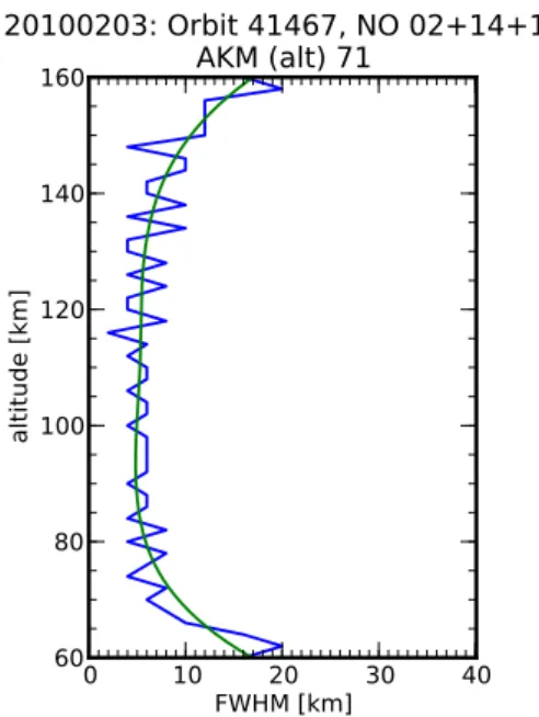
The vertical averaging kernel elements of our retrieval for a particular orbit are shown in Fig. 6. The respective full width at half maximum, fwhm, are shown in Fig. 7. The fwhm is used as a measure of the vertical resolution and is 10 km or better in the range from 70 to 150 km. A vertical resolution of about 5 km is achieved from 80 to 140 km.
0
10
20
30
40
FWHM [km]
60
80
100
120
140
160
altitude [km]
20100203: Orbit 41467, NO 02+14+15
AKM (alt) 71
Fig. 7.FWHM of the altitude averaging kernel matrix elements for a sample orbit (no. 41467, 3 February 2010) as an indicator of vertical resolution.
80 60 40 20 0
20 40 60 80
latitude [deg]
0.1
0.0
0.1
0.2
0.3
AKM
20100203: Orbit 41467, NO 02+14+15
AKM (lat) 106 km
Fig. 8.Latitude averaging kernel matrix elements for a sample orbit (no. 41467, 3 February 2010).
fwhm shown in Fig. 9. In the retrieval runs in this paper, the grid consists of 2.5◦latitude bins, which restricts the fwhm to the resolution within subsequent 2.5◦bins. This makes the horizontal resolution jump between 7.5◦ and 12.5◦ around the true value. The average is obtained by a cubic B-spline fit using a large smoothing constraint, and a similar figure is obtained by using a 13 or 15 point running mean. It shows that the real horizontal resolution, determined by the radia-tive transfer, is quite constant between 60◦S and 60◦N, be-ing that for 9◦.
60 40 20 0 20 40 60
latitude [deg] 6
7 8 9 10 11 12 13 14
FWHM [deg]
20100203: Orbit 41467, NO 02+14+15
AKM (lat) 106 km
Fig. 9.FWHM of the latitude averaging kernel matrix elements for a sample orbit (no. 41467, 3 February 2010). The apparent large variation is due to the grid spacing of 2.5◦. The green line is a smoothed cubic B-spline fit indicating an average latitudinal res-olution of about 9◦.
4.3 Comparison to one-dimensional retrieval
A common approach used in trace gas retrieval consists of using homogeneous atmosphere layers to invert only a sin-gle limb scan, resulting in a vertical profile at one geoloca-tion. This works well when the radiative paths through the atmospheric volumes for each scan are independent of one another, i.e. the distance between limb scans is larger than the optical path for a given tangent height and the gradient in NO is small. NO in the lower thermosphere and upper meso-sphere, however, has a steep horizontal gradient from high to mid-latitudes. Here, the two-dimensional approach allows us to take advantage of the closely spaced limb scans from SCIAMACHY, in particular in the northern polar region. The combined information from the overlapping limb scans along the line-of-sight helps to better represent the strong latitudi-nal gradient. The method is new, and is described in more de-tail in Langowski et al. (2013). To demonstrate the advantage of the 2-D, or more generally tomographic, retrieval over the 1-D retrieval, a comparison is presented.
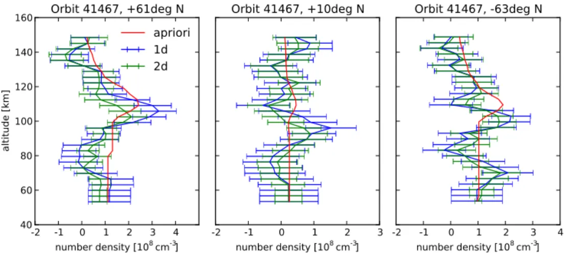
The 1-D version of the retrieval results in a vertical pro-file of the NO number density along a single limb scan. In the 2-D version of the retrieval, the latitude distribution of a limb scan spans three latitude bins of the retrieval grid. To compare those two methods, the number densities of the 2-D result have been interpolated to the limb scan’s latitudes. The vertical profiles in comparison are shown in Fig. 10 together with the a priori input. Results are shown for high northern latitude (61◦N), in the equatorial region (10◦N), and in the southern polar region (63◦S).
-2 -1 0 1 2 3 4
number density [108cm-3]
40 60 80 100 120 140 160
altitude [km]
Orbit 41467, +61deg N
apriori
1d
2d
-2 -1 0 1 2 3
number density [108cm-3]
Orbit 41467, +10deg N
-2 -1 0 1 2 3 4
number density [108cm-3]
Orbit 41467, -63deg N
Fig. 10.Comparison of retrieval methods, 1-D retrieval (blue line), 2-D retrieval (green line), and the respective a priori input (red line) for three geographic regions of the selected sample orbit (no. 41467, 3 February 2010).
are both, differences in the peak altitude and in the absolute value of the density. The 2-D results show a smaller measure-ment error due to the possible influence of neighbouring limb scans in the retrieval. However, to make both methods com-parable, the latitudinal regularisation was switched off for the 1-D version and the vertical parameter was slightly adjusted. This comparison gives confidence in the 2-D retrieval since the results are of the same quality or better than the 1-D re-sults. Thus, it is a valid method to measure the NO content in the middle atmosphere from SCIAMACHY UV spectra. 4.4 Comparison to MIPAS measurements
As MIPAS and SCIAMACHY both fly on Envisat, although viewing in the opposite direction, a direct comparison of the results is possible. Data products from the MIPAS instru-ment (Bermejo-Pantaleón et al., 2011) include the volume mixing ratio (vmr) rather than the number densities of NO. We have converted the MIPAS vmr values to number den-sities using their retrieved temperatures. Retrieved polar NO profiles have a vertical resolution of 5–10 km for highAp
val-ues, and degrade to 10–20 km for lowApconditions. Below
approximately 120 km, total retrieval errors are dominated by instrumental noise. The typical single measurement precision of NO abundances is 10–30% for highApvalues, increasing
to 20–50 % for lowApconditions. Above 120 km, systematic
errors due to uncertainties of the atomic oxygen profile used in the non-LTE modelling are the dominant error source.
We compare the vertical NO columns in the range of 70–140 km from MIPAS to the SCIAMACHY derived re-sults. This is the range of maximal vertical resolution of the SCIAMACHY retrieval. Both instruments have differ-ent vertical resolutions, and both are broad with respect to NO vertical variability. For this reason, column comparisons have been done. This, however, implies merging two differ-ent MIPAS NO products (below 100 km using temperature retrieved at 15 µm and above from a joint T-NO retrieval
80 60 40 20 0 20 40 60 80
latitude [deg] 0.0
0.5 1.0 1.5 2.0 2.5
vc ratio
2008: SCIAMACHY / MIPAS, 43 orbits
Fig. 11.Ratio of SCIAMACHY to MIPAS NO vertical columns (70–140 km), averaged in 20◦latitude bins from 43 coincident or-bits in 2008. The horizontal bars indicate the bins and the vertical bars the 3σconfidence interval.
at 5.3 µm) which may have different biases. Nevertheless, possible inconsistencies related to this merging are consid-ered to have a smaller impact on the column comparisons than the different vertical resolutions would have on pro-file comparisons. For our comparison, the vertical column ratios (SCIAMACHY/MIPAS) for orbits, where both instru-ments scanned the upper atmosphere are binned into 20◦
lat-itude bins and are shown for 2008 in Fig. 11 and for 2009 in Fig. 12. The MIPAS measurements are confined to those for daylight limb scans, selected by using the criterion that the solar zenith angle must be smaller than 95◦, since the com-parison goes down to 70 km.
80 60 40 20 0 20 40 60 80 latitude [deg]
0.0 0.5 1.0 1.5 2.0 2.5
vc ratio
2009: SCIAMACHY / MIPAS, 73 orbits
Fig. 12.Ratio of SCIAMACHY to MIPAS NO vertical columns (70–140 km), averaged in 20◦latitude bins from 73 coincident or-bits in 2009. The horizontal bars indicate the bins and the vertical bars the 3σconfidence interval.
1 Jan
2009
1 Jan
2010
1 Jan
2011
date
0
2
4
6
8
10
nu
mb
er
de
nsi
ty
[10
7
cm
-3]
daily mean NO density, 5S-5N, 106 km
SCIAMACHY
MIPAS
NOEM model
Fig. 13. Equatorial daily mean nitric oxide number density at 106 km, SCIAMACHY MLT (black) and MIPAS UA (blue) com-pared to the NOEM model (red) (Marsh et al., 2004) based on SNOE data (Barth et al., 2003). The grey shaded area shows the 3σ confidence interval of the SCIAMACHY daily means and the blue triangles indicate coincident SCIAMACHY MLT and MIPAS UA measurement days.
the MIPAS results, except for higher northern latitudes (in particular in 2008). One possible explanation might be the deficit of simultaneous measurements in that region. There are four times (2009) to ten times (2008) as many coincident points at middle to low latitudes as in the 80◦bins. This ratio
is about two in the−80◦ bins and although both retrievals use a similar regularisation, different biases can result when dealing with unavailable direct measurements. The a priori constraint in the SCIAMACHY retrieval,Sa, bends the
so-lution into the direction of the number density given by the model. In contrast, the MIPAS regularisation matrices have the effect of using the profile shape as a constraint for the
1 Jan
2009
1 Jan
2010
1 Jan
2011
date
0
5
10
15
20
25
30
35
40
nu
mb
er
de
nsi
ty
[10
7
cm
-3]
daily mean NO density, 60N-70N, 106 km
SCIAMACHY
MIPAS
NOEM model
Fig. 14.Auroral daily mean nitric oxide number density at 106 km, SCIAMACHY MLT (black) and MIPAS UA (blue) compared to the NOEM model (red) (Marsh et al., 2004) based on SNOE data (Barth et al., 2003). The grey shaded area shows the 3σconfidence interval of the SCIAMACHY daily means and the blue triangles indicate coincident SCIAMACHY MLT and MIPAS UA measurement days.
lution. This may explain part of the disagreement, but further research is required to establish the origin of the differences quantitatively.
4.5 Number density time series
For the MLT observations from July 2008 until March 2011, the NO number density at 106 km in the equatorial region (5◦S–5◦N) is shown in Fig. 13, in the auroral region (60◦N–
66◦N) in Fig. 14. We compare the results for NO, retrieved from SCIAMACHY with those from MIPAS and those from the NOEM model (Marsh et al., 2004) which is derived from SNOE measurements (Barth et al., 2003).
The patterns of the SCIAMACHY NO are similar to those from NOEM. However, the NOEM results are systematically higher than the SCIAMACHY data. This disagreement is largest in 2008 and 2009, during the deep solar minimum, when also the geomagnetic activity was very low; in 2010, when both solar and geomagnetic activity were beginning to increase again, the agreement is better. Nearly perfect agree-ment is reached in 2011 at high latitudes. The consistency among the MIPAS and SCIAMACHY data may hint at as-sumptions within the NOEM model, which was derived from SNOE observations during a period of continuous high solar and geomagnetic activity (1998–2000).
5 Conclusions
from the SCIAMACHY instrument aboard Envisat. The method is adapted from earlier work (cf. Scharringhausen et al., 2008b, a) and was extended to use the gamma bands of NO and the UV spectra of SCIAMACHY’s special MLT limb scans. The retrieval method is an adapted version of the MIPAS retrieval algorithm to be found in von Clarmann et al. (2003) and Funke et al. (2005b). Using 3-D ray tracing, a 2-D retrieval grid, and regularisation with respect to altitude and latitude yields the NO density for half an orbit simulta-neously for the altitude range from 60–160 km.
The retrieval of NO number densities from the fit of calcu-lated spectra for the NO gamma bands gives yields NO data, which are consistent with previous measurements from Barth et al. (2003) and Minschwaner et al. (2004). A first compari-son shows that they are also in reacompari-sonable agreement between 60◦N and 60◦S with the measurements of the MIPAS
instru-ment on board the same satellite for the orbits where both instruments scanned the upper atmosphere (50–150 km). For low geomagnetic activity (lowAp) in 2008–2010, we obtain
a vertical resolution of 5–10 km in the altitude range 70– 150 km and a horizontal resolution of about 9◦.
The current approach is successful in retrieving the NO number densities in the mesosphere and lower thermosphere with SCIAMACHY MLT limb scans. The results are in rea-sonable agreement with previous measurements from other instruments and provide an almost continuous data source for NO in that region from 2008 to 2012. The comparison to the empirical NOEM model shows that the largest devi-ations occur at times of low solar activity. The consistency among the measurements, however, indicates that the model assumptions, derived from NO observations at times of high solar activity, need further investigation. In the future, lati-tudinal and longilati-tudinal resolution can be further improved by using two-dimensional detector arrays on new missions. Similarly, such detectors provide longer integration times for the study of weak signals,
Continuous measurements in the MLT region over a long time span are essential to improve our knowledge and under-standing of the connection between solar activity and ther-mospheric NO. This is an important link in the atther-mospheric system controlling stratospheric ozone and thereby impact-ing on climate. Observations in the middle atmosphere also allow to follow the NO produced from solar particles in the region around 100 km downwards during the polar winter, in particular during extraordinary atmospheric events such as stratospheric warmings. This facilitates the attribution of an-thropogenic influences on the atmospheric composition from the changes resulting from the varying solar activity during a solar cycle. This is of particular value for the validation of climate models with respect to the production of NOxand its
transport.
Acknowledgements. S. Bender and M. Sinnhuber thank the
Helmholtz-society for funding this project under the grant number
VH-NG-624. The IAA team (M. López-Puertas and B. Funke) was supported by the Spanish MINECO under grant AYA2011-23552 and EC FEDER funds. The SCIAMACHY project was funded by German Aerospace (DLR), the Dutch Space Agency, SNO, and the Belgium ministry. ESA funded the Envisat project. The University of Bremen as Principal Investigator has led the scientific support and development of SCIAMACHY and the scientific exploitation of its data products. We acknowledge support by Deutsche Forschungsgemeinschaft and Open Access Publishing Fund of Karlsruhe Institute of Technology.
The service charges for this open access publication have been covered by a Research Centre of the Helmholtz Association.
Edited by: H. Worden
References
Barth, C. A., Mankoff, K. D., Bailey, S. M., and Solomon, S. C.: Global observations of nitric oxide in the thermosphere, J. Geo-phys. Res., 108, 1027, doi:10.1029/2002JA009458, 2003. Bermejo-Pantaleón, D., Funke, B., López-Puertas, M.,
García-Comas, M., Stiller, G. P., von Clarmann, T., Linden, A., Grabowski, U., Höpfner, M., Kiefer, M., Glatthor, N., Kellmann, S., and Lu, G.: Global observations of thermospheric tempera-ture and nitric oxide from MIPAS spectra at 5.3 µm, J. Geophys. Res., 116, A10313, doi:10.1029/2011JA016752, 2011.
Bovensmann, H., Burrows, J. P., Buchwitz, M., Frerick, J., Noël, S., Rozanov, V. V., Chance, K. V., and Goede, A. P. H.: SCIAMACHY: Mission Objectives and Measure-ment Modes, J. Atmos. Sci., 56, 127–150, doi:10.1175/1520-0469(1999)056<0127:SMOAMM>2.0.CO;2, 1999.
Burrows, J. P., Hölzle, E., Goede, A. P. H., Visser, H., and Fricke, W.: SCIAMACHY – scanning imaging absorption spectrome-ter for atmospheric chartography, Acta Astronaut., 35, 445–451, doi:10.1016/0094-5765(94)00278-T, 1995.
Callis, L. B., Natarajan, M., Evans, D. S., and Lambeth, J. D.: Solar atmospheric coupling by electrons (SOLACE): 1. Effects of the May 12, 1997 solar event on the middle atmosphere, J. Geophys. Res., 103, 28405–28419, doi:10.1029/98JD02408, 1998. Chance, K. and Kurucz, R.: An improved high-resolution solar
ref-erence spectrum for earth’s atmosphere measurements in the ul-traviolet, visible, and near infrared, J. Quant. Spectrosc. Ra., 111, 1289–1295, doi:10.1016/j.jqsrt.2010.01.036, 2010.
Cleary, D. D.: Daytime High-Latitude Rocket Observations of the NO γ, δ, and ε Bands, J. Geophys. Res., 91, 11337–11344, doi:10.1029/JA091iA10p11337, 1986.
Earls, L. T.: Intensities in 25−26 Transitions in Diatomic Molecules, Phys. Rev., 48, 423–424, doi:10.1103/PhysRev.48.423, 1935.
Eparvier, F. G. and Barth, C. A.: Self-Absorption Theory Applied to Rocket Measurements of the Nitric Oxide (1, 0)γ Band in the Daytime Thermosphere, J. Geophys. Res., 97, 13723–13731, doi:10.1029/92JA00993, 1992.
Funke, B., López-Puertas, M., Gil-López, S., von Clarmann, T., Stiller, G. P., Fischer, H., and Kellmann, S.: Downward transport of upper atmospheric NOx into the polar
strato-sphere and lower mesostrato-sphere during the Antarctic 2003 and Arctic 2002/2003 winters, J. Geophys. Res., 110, D24308, doi:10.1029/2005JD006463, 2005a.
Funke, B., López-Puertas, M., von Clarmann, T., Stiller, G. P., Fischer, H., Glatthor, N., Grabowski, U., Höpfner, M., Kell-mann, S., Kiefer, M., Linden, A., Mengistu Tsidu, G., Milz, M., Steck, T., and Wang, D. Y.: Retrieval of stratospheric NOxfrom
5.3 and 6.2 µm nonlocal thermodynamic equilibrium emissions measured by Michelson Interferometer for Passive Atmospheric Sounding (MIPAS) on Envisat, J. Geophys. Res., 110, D09302, doi:10.1029/2004JD005225, 2005b.
Kerzenmacher, T., Wolff, M. A., Strong, K., Dupuy, E., Walker, K. A., Amekudzi, L. K., Batchelor, R. L., Bernath, P. F., Berthet, G., Blumenstock, T., Boone, C. D., Bramstedt, K., Brogniez, C., Brohede, S., Burrows, J. P., Catoire, V., Dodion, J., Drummond, J. R., Dufour, D. G., Funke, B., Fussen, D., Goutail, F., Grif-fith, D. W. T., Haley, C. S., Hendrick, F., Höpfner, M., Huret, N., Jones, N., Kar, J., Kramer, I., Llewellyn, E. J., López-Puertas, M., Manney, G., McElroy, C. T., McLinden, C. A., Melo, S., Mikuteit, S., Murtagh, D., Nichitiu, F., Notholt, J., Nowlan, C., Piccolo, C., Pommereau, J.-P., Randall, C., Raspollini, P., Ri-dolfi, M., Richter, A., Schneider, M., Schrems, O., Silicani, M., Stiller, G. P., Taylor, J., Tétard, C., Toohey, M., Vanhellemont, F., Warneke, T., Zawodny, J. M., and Zou, J.: Validation of NO2and
NO from the Atmospheric Chemistry Experiment (ACE), At-mos. Chem. Phys., 8, 5801–5841, doi:10.5194/acp-8-5801-2008, 2008.
Langowski, M., Sinnhuber, M., Aikin, A. C., von Savigny, C., and Burrows, J. P.: Retrieval algorithm for densities of mesospheric and lower thermospheric metal and ion species from satellite borne limb emission signals, Atmos. Meas. Tech. Discuss., 6, 4445–4509, doi:10.5194/amtd-6-4445-2013, 2013.
Luque, J. and Crosley, D. R.: Transition probabilities and elec-tronic transition moments of the A26+–X25 and D26+– X25systems of nitric oxide, J. Chem. Phys., 111, 7405–7415, doi:10.1063/1.480064, 1999.
Marsh, D. R., Solomon, S. C., and Reynolds, A. E.: Empirical model of nitric oxide in the lower thermosphere, J. Geophys. Res., 109, A07301, doi:10.1029/2003JA010199, 2004.
Minschwaner, K., Bishop, J., Budzien, S. A., Dymond, K. F., Siskind, D. E., Stevens, M. H., and McCoy, R. P.: Middle and upper thermospheric odd nitrogen: 2. Measurements of nitric ox-ide from Ionospheric Spectroscopy and Atmospheric Chemistry (ISAAC) satellite observations of NOγ band emission, J. Geo-phys. Res., 109, A01304, doi:10.1029/2003JA009941, 2004. NGDC and NOAA: Space Physics Interactive Data Resource
(SPIDR), available at: http://spidr.ngdc.noaa.gov/spidr/ (last ac-cess: 17 February 2012), 2011.
Picone, J. M., Hedin, A. E., Drob, D. P., and Aikin, A. C.: NRLMSISE-00 empirical model of the atmosphere: Statistical comparisons and scientific issues, J. Geophys. Res., 107, 1468, doi:10.1029/2002JA009430, 2002.
Piper, L. G. and Cowles, L. M.: Einstein coefficients and transition moment variation for the NO(A26+–X25) transition, J. Chem. Phys., 85, 2419–2422, doi:10.1063/1.451098, 1986.
Randall, C. E., Harvey, V. L., Siskind, D. E., France, J., Bernath, P. F., Boone, C. D., and Walker, K. A.: NOxdescent in the
Arc-tic middle atmosphere in early 2009, Geophys. Res. Lett., 36, L18811, doi:10.1029/2009GL039706, 2009.
Rodgers, C. D.: Retrieval of atmospheric temperature and composi-tion from remote measurements of thermal radiacomposi-tion, Rev. Geo-phys., 14, 609–624, doi:10.1029/RG014i004p00609, 1976. Schadee, A.: The formation of molecular lines in the solar spectrum
(Errata: 17 537), B. Astron. Inst. Neth., 17, 311–357, 1964. Scharringhausen, M., Aikin, A. C., Burrows, J. P., and
Sinnhu-ber, M.: Global column density retrievals of mesospheric and thermospheric MgI and MgII from SCIAMACHY limb and nadir radiance data, J. Geophys. Res., 113, D13303, doi:10.1029/2007JD009043, 2008a.
Scharringhausen, M., Aikin, A. C., Burrows, J. P., and Sinnhu-ber, M.: Space-borne measurements of mesospheric magnesium species – a retrieval algorithm and preliminary profiles, At-mos. Chem. Phys., 8, 1963–1983, doi:10.5194/acp-8-1963-2008, 2008b.
Sheese, P. E., Gattinger, R. L., Llewellyn, E. J., Boone, C. D., and Strong, K.: Nighttime nitric oxide densities in the Southern Hemisphere mesosphere–lower thermosphere, Geophys. Res. Lett., 38, L15812, doi:10.1029/2011GL048054, 2011.
Sinnhuber, M., Kazeminejad, S., and Wissing, J. M.: Interannual variation of NOx from the lower thermosphere to the upper stratosphere in the years 1991–2005, J. Geophys. Res., 116, A02312, doi:10.1029/2010JA015825, 2011.
Sinnhuber, M., Nieder, H., and Wieters, N.: Energetic Particle Pre-cipitation and the Chemistry of the Mesosphere/Lower Ther-mosphere, Surv. Geophys., 33, 1281–1334, doi:10.1007/s10712-012-9201-3, 2012.
Siskind, D. E., Nedoluha, G. E., Randall, C. E., Fromm, M., and Russell, J. M.: An assessment of southern hemi-sphere stratospheric NOx enhancements due to transport from the upper atmosphere, Geophys. Res. Lett., 27, 329–332, doi:10.1029/1999GL010940, 2000.
Stevens, M. H.: Nitric Oxideγ Band Fluorescent Scattering and Self-Absorption in the Mesosphere and Lower Thermosphere, J. Geophys. Res., 100, 14735–14742, doi:10.1029/95JA01616, 1995.
Stevens, M. H., Siskind, D. E., Hilsenrath, E., Cebula, R. P., Leitch, J. W., Russell, J. M., and Gordley, L. L.: Shuttle solar backscat-ter UV observations of nitric oxide in the upper stratosphere, mesosphere, and thermosphere: Comparisons with the Halo-gen Occultation Experiment, J. Geophys. Res., 102, 9717–9727, doi:10.1029/97JA00326, 1997.
Tatum, J. B.: The Interpretation of Intensities in Diatomic Molecular Spectra, Astrophys. J. Suppl., 14, 21–55, doi:10.1086/190149, 1967.