SRef-ID: 1432-0576/ag/2004-22-3383 © European Geosciences Union 2004
Annales
Geophysicae
Effect of planetary waves on cooling the upper mesosphere and
lower thermosphere by the CO
2
15-
µ
m emission
G. M. Shved, V. P. Ogibalov, and A. I. Pogoreltsev
Dept. of Atmosph. Phys., Inst. of Phys., St. Petersburg State Univ., St. Petersburg-Petrodvorets 198504, Russia Received: 22 December 2003 – Revised: 17 June 2004 – Accepted: 24 June 2004 – Published: 3 November 2004
Abstract. The steady-state 2-D linearized model of global-scale waves, calibrated according to available observations, is used to evaluate planetary-wave perturbations of temper-ature from the surface up to the height of about 165 km. The maximum order of perturbation amplitudes in the up-per mesosphere and lower thermosphere is found to be 15 K for the ultra-fast Kelvin wave (UFKW) of the 3.5-day period, 8 K for the 10-day wave, 5 K for the 2- and 16-day waves, and 2 K for the 5-day wave. The wave-caused variation in heat in-flux in the CO215-µm band, averaged over the wave period, depends on both the amplitude of temperature and tempera-ture profile in the atmosphere unperturbed by the wave. An additional increase in radiative cooling is the prevailing ef-fect of planetary waves in the upper mesosphere and lower thermosphere. The UFKW results in an increasing cooling rate up to∼0.1 of the cooling rate in the unperturbed atmo-sphere. The tangible contributions of the 2-, 10-, and 16-day waves are questionable. The contribution of the 5-day wave is negligible.
Key words. Meteorology and atmospheric dynamics (waves and tides; radiative processes)
1 Introduction
The main mechanism for the cooling of the atmosphere up to the heights of 110–120 km is infrared radiative cooling (e.g. Roble, 1995). In the upper mesosphere/lower thermosphere (UMLT) region between ∼70 and 120 km the CO215-µm emission dominates in infrared cooling (e.g. Fomichev et al., 1986).
The population of atomic and molecular states, which give the atmospheric infrared emission, is controlled by thermal atomic/molecular collisions, either totally (local thermody-namic equilibrium (LTE) for a state of interest) or partially (non-LTE). The efficiency of collisional excitation increases with atmospheric temperature. As a result the rate of ra-diative cooling depends on temperature. This dependence
Correspondence to:G. M. Shved
is very complicated since the radiative influx of heat at an atmospheric level is determined as the difference between absorbed energy of the radiation emitted at other levels and energy emitted at the level considered. Thus, the radiative cooling rate depends in a complicated way on the features of vertical temperature profile in a layer of the atmosphere.
The observations show a strong spatial-temporal variabil-ity of temperature profile in the upper and middle atmo-sphere. Any temperature profile observed can be treated as the superposition of a smoothed climatological profile chang-ing with latitude and season and of a perturbation. The per-turbations are caused by waves and eddies. The scales of waves and eddies are extremely varied in time and space. That is why the evaluations of the radiative cooling rate are made as a rule for climatological profiles of temperature (e.g. Dickinson, 1984; Fomichev et al., 1986; Khvorostovskaya et al., 2002).
Ignoring the aforementioned perturbations in temperature results in an error in estimating the radiative cooling rate. For the first time, the effect of temperature perturbations in the UMLT region on this rate was analyzed by Kutepov and Shved (1978), who tested an influence of wave-caused per-turbations on cooling by the CO2 15-µm emission. Later, Fomichev et al. (1986) have shown an additional cooling in the 70–110 km layer, which is produced due to the effect of the 24- and 12-hour tides and internal gravity waves on the CO215-µm, O39.6-µm, and H2O rotational emissions.
Here we estimate the effect on UMLT radiative cooling of temperature perturbations caused by planetary waves (atmo-spheric normal modes and equatorial waves) (e.g. Ahlquist, 1985; Andrews et al., 1987). There are many modes of the planetary waves, which differ in zonal number and the pe-riod of the wave. We consider the modes which perturb the middle atmosphere most strongly. The 2-, 5-, 10-, and 16-day waves among normal modes and the ultra-fast Kelvin wave (UFKW) among equatorial waves have been therefore selected for analyzing.
-90 -60 -30 0 30 60 90
Latitude (deg) 10
11 12 13 14 15 16 17 18
ln
[1
000/
p(
h
P
a
)]
-90 -60 -30 0 30 60 90
Latitude (deg) 10
11 12 13 14 15 16 17 18
a)
b)
Fig. 1.Relationship between geometrical (in km) and log-pressure coordinates in the UMLT region for 16 March(a)and 1 July(b)from the MSISE-90 model (Hedin, 1991).
Ahlquist, 1985). That is why we estimate only a maxi-mum order-of-magnitude for the wave perturbation of radia-tive cooling rate. Taking into account the only CO215-µm emission is sufficient in our estimating, since this emission dominates in UMLT radiative cooling.
2 Planetary wave models
The steady-state 2-D linearized model of global-scale waves, described by Pogoreltsev (1996, 1999, 2001), has been used in this study to simulate wave perturbations of temperature
T. The model domain extends from the South Pole to the North Pole and from the surface up to the height of about 165 km. The planetary waves modeled are forced by vertical motions at the lower boundary with an arbitrary amplitude of vertical velocity. The solutions obtained are calibrated, i.e. the wave amplitude modeled is multiplied by an appropriate factor to reproduce the amplitudes of planetary-wave pertur-bations of the temperature, geopotential height, and/or wind, which are observed in the middle atmosphere.
The amplitude of the planetary wave in the UMLT region depends mainly on background zonal wind which varies with season. We have evaluated the wave perturbations ofT for two cases which differ considerably in the latitude-height distribution of background wind. We have taken the con-ditions of 1 July as characteristic for summer/winter. For spring/autumn the conditions of 16 March have been taken, since the zonal wind distribution near this date results in the strongest amplitude in the UMLT region for longer-period planetary waves. The springtime transition in atmospheric circulation of the Northern Hemisphere occurs near this date.
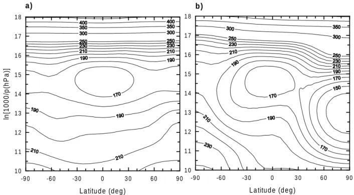
The background temperature and background zonal wind ve-locity have been taken from the MSISE-90 (Hedin, 1991) and HWM-93 (Hedin et al., 1996) empirical models, respec-tively. Figure 1 shows the relationship between geometrical heightzand dimensionless log-pressure height ln(1000/p), where p is the pressure in hPa. Figures 2 and 3 plot the background temperature and wind, respectively.
To reproduce the realistic conditions, the solution was cal-ibrated using the observed amplitudes of the considered plan-etary waves. The amplitude of temperature perturbations,
-9 0 -6 0 -3 0 0 3 0 6 0 9 0
L a titu de (d e g ) 1 0
1 1 1 2 1 3 1 4 1 5 1 6 1 7 1 8
ln
[10
00
/p
(h
P
a
)]
-9 0 -6 0 -3 0 0 3 0 6 0 9 0
L a titu d e (d e g ) 1 0
1 1 1 2 1 3 1 4 1 5 1 6 1 7 1 8
a)
b)
Fig. 2. Latitude-height distributions of background temperature in Kelvin in the UMLT region for 16 March(a)and 1 July(b)from the MSISE-90 model (Hedin, 1991).
-90 -60 -30 0 30 60 90
Latitude (deg)
02 4 6 8 10 12 14 16 18
ln
[1
0
0
0
/p
(h
P
a
)]
a)
-90 -60 -30 0 30 60 90
Latitude (deg)
02 4 6 8 10 12 14 16 18
ln
[1
0
0
0
/p
(h
P
a
)]
b)
Fig. 3.Latitude-height distributions of velocity of background zonal wind in m/s (positive eastward) for 16 March(a)and 1 July(b)from the HWM-93 model (Hedin et al., 1996), used in simulating the planetary waves.
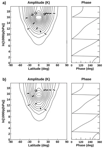
Figures 4–8 show the latitude-height distributions ofδT
and examples of phase progression for the planetary waves considered. The UFKW propagation results in the strongest perturbations ofT in the UMLT region (near the equator), providingδT up to∼15 K. Next, in order of magnitude, is
-90 -60 -30 0 30 60 90
Latitude (deg)
Amplitude (K)
0 2 4 6 8 10 12 14 16 18
ln
[1
0
0
0
/p
(h
P
a
)]
a)
0 120 240 360 Phase (deg)
Phase
-90 -60 -30 0 30 60 90
Latitude (deg)
Amplitude (K)
0 2 4 6 8 10 12 14 16 18
ln
[1
0
0
0
/p
(h
P
a
)]
b)
0 120 240 360 Phase (deg)
Phase
Fig. 4. Latitude-height distribution of amplitude (left) and phase (right) of temperature perturbations for the ultra-fast Kelvin wave for 16 March(a)and 1 July(b). The phases are shown at the equa-tor.
3 Method for calculating cooling
To evaluate heat influx in the CO215-µm band,hr, in the
UMLT region, the non-LTE for vibrational states of CO2 molecules should be taken into account (L´opez-Puertas and Taylor, 2001). The computational code used for evaluating
hr is outlined by Ogibalov et al. (2000). The code is based
on an optical model presented by Shved et al. (1998). The set of inelastic collisional transitions and their rate constants are also borrowed from Shved et al. (1998). The one exception is for the rate constant for quenching the CO2(0110) state by O atoms, which is taken from the recent laboratory measure-ment of Khvorostovskaya et al. (2002). The profiles of the O mixing ratio and the only profile of the CO2mixing ratio are borrowed from the models of Llewellyn and McDade (1996) and Shved et al. (1998), respectively. The latitude-height dis-tributions of climatological temperature,T0(z,ϕ), whereϕis the latitude, are taken from the MSISE-90 as for the plane-tary wave models.
To evaluatehr, we specify temperature as
T (z, ϕ, t )=T0(z, ϕ)+δT (z, ϕ)sin[2π t /τ+α(z, ϕ)], (1)
-90 -60 -30 0 30 60 90
Latitude (deg)
Amplitude (K)
0 2 4 6 8 10 12 14 16 18
ln
[1
0
0
0
/p
(h
P
a
)]
a)
0 120 240 360 Phase (deg)
Phase
-90 -60 -30 0 30 60 90
Latitude (deg)
Amplitude (K)
0 2 4 6 8 10 12 14 16 18
ln
[1
0
0
0
/p
(h
P
a
)]
b)
0 120 240 360 Phase (deg)
Phase
Fig. 5.As in Fig. 4, but for the 5-day wave. The phases are shown at 45◦S(a)and 45◦N(b).
wheret is the time,τ andαare the period and phase angle of the wave, respectively. We search for heat influx averaged overτ:
hr(z, ϕ) =
1
τ
τ
Z
0
hr(z, ϕ, t ) dt . (2)
(Here and below, the over-bar denotes an average overτ.) The calculation of the latitude-height distribution of heat in-flux forT0(z,ϕ),hr,0(z,ϕ), makes it possible to find a
wave-caused change in the heat influx:
1hr(z, ϕ) = hr(z, ϕ) −hr,0(z, ϕ) . (3) Figure 9 plotshr,0(z,ϕ) for 16 March and 1 July.
4 Theory
In this section we present an explanation for the effect of planetary waves on heat influx in the CO215-µm band. For clarity of explanation we simplify the structure of the band in comparison with its actual structure used in the computa-tional code for evaluatinghr (see Sect. 3). Our consideration
-90 -60 -30 0 30 60 90 Latitude (deg) Amplitude (K) 0 2 4 6 8 10 12 14 16 18 ln [1 0 0 0 /p (h P a )] a)
0 120 240 360 Phase (deg)
Phase
-90 -60 -30 0 30 60 90
Latitude (deg) Amplitude (K) 0 2 4 6 8 10 12 14 16 18 ln [1 0 0 0 /p (h P a )] b)
0 120 240 360 Phase (deg)
Phase
Fig. 6.As in Fig. 4, but for the 10-day wave. The phases are shown at 45◦N(a)and 45◦S(b).
main isotop12C16O2.This transition dominates absolutely in
radiative cooling of the lower thermosphere (L´opez-Puertas and Taylor, 2001).
The heat influx in the band is a result of molecular colli-sions which are accompanied by the transfer of vibrational energy to and from translational energy. Ignoring small dis-parities in energy of vibrational quanta corresponding differ-ent rovibrational transitions of the band,hr per one molecule
of air
hr =hν0cCO2(W2C21−W1C12), (4) wherehis Plank’s constant,ν0is the frequency of vibrational transition, cM is the volume mixing ratio for the gas
con-stituent M of the atmosphere,Wi is the probability of CO2
molecules (population) to be in the vibrational statei, and
Cij is the number of vibrational transitionsi→j in a unit
time per one molecule in the initial statei. Here, the states 0000 and 0110 are denoted by the subscripts 1 and 2, respec-tively. The coefficientCij is expressed as
Cij =n
X
M
kij,McM, (5)
wherenis the total concentration of molecules in the atmo-sphere, andkij,M is the rate constant for vibrational
transi--90 -60 -30 0 30 60 90
Latitude (deg) Amplitude (K) 0 2 4 6 8 10 12 14 16 18 ln [1 0 0 0 /p (h P a )] a)
0 120 240 360 Phase (deg)
Phase
-90 -60 -30 0 30 60 90
Latitude (deg) Amplitude (K) 0 2 4 6 8 10 12 14 16 18 ln [1 0 0 0 /p (h P a )] b)
0 120 240 360 Phase (deg)
Phase
Fig. 7.As in Fig. 4, but for the 16-day wave. The phases are shown at 45◦N(a)and 45◦S(b).
-90 -60 -30 0 30 60 90
Latitude (deg) Amplitude (K) 0 2 4 6 8 10 12 14 16 18 ln [1 0 0 0 /p (h P a )]
0 40 80 120
Phase (deg)
Phase
Fig. 8.As in Fig. 4, but for the 2-day wave and only for 1 July. The phase is shown at 45◦N.
-90 -60 -30 0 30 60 90
Latitude(deg) 10
11 12 13 14 15 16 17 18
ln
[1
000/
p(
h
P
a
)]
-90 -60 -30 0 30 60 90
Latitude (deg) 10
11 12 13 14 15 16 17 18
a)
b)
-35
Fig. 9.Latitude-height distributions of heat influx in the CO215-µm band in K/day in the UMLT region for 16 March(a)and 1 July(b), based on vertical profiles of temperature from the MSISE-90 model (Hedin, 1991). The dashed isolines correspond to atmospheric heating.
equation
g1k12,M = g2k21,Mexp
−hν0 kT
, (6)
wherekis the Boltzmann constant, andgi is the degeneracy
for a statei. Here,g1=1, andg2=2.
The non-LTE for the CO2 15-µm band occurs above 70 km (Khvorostovskaya et al., 2002). This means that ra-diative transitions are involved in the formation of the 0110 state population in the UMLT region, along with collisional transitions. Ignoring a small contribution by the induced pho-ton emission to the state population,W1andW2appear to be related by the equation
W2(A21+C21)=W1(B12ρr +C12), (7) where A21 and B12 are the Einstein coefficients of spon-taneous photon emission and photon absorption by CO2 molecules, respectively, andρr is the “effective” density of
photons (see below) for the 0000–0110 transitions. It is appropriate to consider two limiting cases:
A. The LTE case of dominating collisional transitions in the population formation (C21≫A21,C12≫B12ρr). In this
case, in accordance with Eqs. (4), (6), and (7), familiar ex-pressions are valid: Boltzmann’s law for state populations,
W2
W1
= g2 g1
exp
−hν0 kT
, (8)
and the expression forhr,
hr = hν0cCO2W1
B12ρr−
g2
g1
A21exp
−hν0 kT
. (9)
B. The case of dominating radiative transitions in the population formation (A21≫C21,B12ρr≫C12). In this case,
W2
W1
= B12ρr A21
, (10)
and
hr =
hν0cCO2W1C21 A21
B12ρr−
g2
g1
A21exp
−hν0 kT
. (11) It should be noted that the terms which represent the receipts and losses of heat influx, in every limiting case, are pro-portional to the same expressionsB12ρr and (g2/g1)A21exp (−hν0/kT), respectively. These expressions are combined in the square brackets in Eqs. (9) and (11).
The “effective” density of photons, ρr, is the sum over
band lines of the products of the photon’s density in a line by its relative strength in the band. The band lines considered differ in both the rotational quantum numberJ in the lower vibrational state of 0000–0110 transition and the belonging to a band branch denoted by the number1J=J′−J, where
J′is the rotational quantum number in the upper vibrational state. The P-, Q- and R-branches are numbered sequentially as 1J=−1, 0, and 1. According to Shved et al. (1984), the relative strength of the line is approximated by the prod-uctc1JwJ(T ), wherec−1=c1=1/4andc0=1/2,wJ(T )is the
Boltzmann probability of finding a linear molecule in the ro-tational stateJ,
wJ(T ) =
hBr
kT (2J+1) exp
−hBrJ (J+1) kT
, (12)
We use the monochromatic approximation in the radiative transfer theory, since the shape of the line contour is unre-lated to the explanation considered. Then, the radiance in photons for a line (J,1J) and a direction of radiative energy flux can be written as
IJ,1J = c1JA21 ∞ Z
0
dl cCO2 (l) n (l) W2(l) wJ+1J[T (l)]
exp
−c1JB12
l
Z
0
dl′cCO2 l ′
n l′
W1 l′wJT l′
, (13)
wherel is the length along a ray trajectory from the spatial point considered, andρr can be written as
ρr =
1
c
X
J,1J
c1JwJ[T (0)]
Z
(4π )
dω IJ,1J , (14)
wherecis the speed of light, and the integral is taken over the total solid angle.
Since the atmosphere is open to space, the atmospheric in-frared emission cools it. However, the inin-frared emission can also heat in the vicinity of a strong minimum in a vertical profile ofT, as shown in Fig. 9b. This infrared heating is caused by the following reasons, see Eq. (9) and Eq. (11). TheT-dependence of heat losses is determined by the expo-nential function exp(−hν0/kT). That is why the heat losses decrease strongly near the T minimum. The heat receipts are proportional toρr. Those decrease near theT minimum
much less, sinceρris formed by emission from a layer of the
atmosphere.
As is seen from Eq. (4), the wave-caused perturbations in
T impact onhr via theT-dependences ofk12,M,k21,M,W1,
andW2. However, the T variations of W1 are negligible, since the magnitude ofW1 is little different from 1 at at-mospheric temperatures. The quenching of the 0110 state by O atoms dominates in the thermosphere. That is grad-ually substituted by quenching during the CO2(0110)−N2 and CO2(0110)−O2 collisions with a decrease in z. The
T-dependence of k21,O is weak (Khvorostovskaya et al., 2002). However, those of k21,N2 and k21,O2 are tangible (e.g. Shved et al., 1998), though they are much weaker than theT-dependence represented by the factor exp (−hν0/kT). Hence, in accordance with Eq. (6), this factor governs mainly the T-dependence of k21,M. From Eqs. (7) and
(12)−(14), the T-dependence of W2 is very complicated. First, theT-dependences of the rate constantsk21,M, factor
exp (−hν0/kT), and function wJ (T )contribute to it.
Sec-ond,W2 is determined viaρr byT in a layer of the
atmo-sphere.
Since the factor exp (−hν0/kT) is nonlinear inT, its av-eraging overτ results in
exp (−hν0/ kT ) > exp (−hν0/ kT0) (15)
at atmospheric temperatures considered, ifT in Eq. (15) is given by Eq. (1) withδT≪T0. That is why the wave-caused perturbations lead universally to an increase in heat losses.
As is seen from Eqs. (9) and (11), the wave-caused pertur-bations in heat receipts are determined byρr averaged over
τ ,
ρr =
1
c
X
J,1J
c1J
wJ[T (0)] Z
(4π )
dω IJ,1J
. (16) From Eq. (16), the wave impacts on the population of rota-tional states and the photon density in lines in spatial point considered. However, the photon density, in accordance with Eq. (13), is the resultant effect of the wave on a layer of the atmosphere that makes the analysis of the wave impact on heat receipts difficult. Two inferences about wave effects on heat receipts can yet be made. First of all, due to a smooth-ing effect of integratsmooth-ing in Eq. (13) along a ray trajectory, the stronger that the phase of the wave varies withz,the weaker the wave-caused perturbations are inIJ,1J. Secondly, one
can understand the way in which the wave-caused local per-turbation in the rotational state populations acts on heat re-ceipts. As is seen from Eq. (12), an increase in T results in a nonlinear rise of the probabilitieswJ for large numbers
J at the decrease of ones for small numbersJ. This leads to enhancing of the radiation absorption in weak lines (large
J ) and to attenuating that in strong lines (smallJ ). From Eq. (13), the weaker the line, the farther from the height level under consideration the radiation absorbed is formed. Since the optical depth of the thermosphere in the lines of the CO2 15-µm band is less than one, the UMLT photon density in the band is mainly formed by the upward radiation. The rise ofT
down from the mesopause results in an associated increase in the relative population of 0110 state,W2/W1(Ogibalov et al., 1998; L´opez-Puertas and Taylor, 2001). Thus, the weaker a line, the moreW2/W1in the layer forming upward radiation. So, it is due to weak lines that the wave-caused perturbations lead to an increase in radiation absorption in the band at the height level under consideration and correspondingly to the rise in the UMLT heat receipts averaged overτ.
For the sake of discussion in Sect. 5, the following should be noted. As indicated above, there are two features in the lower thermosphere. First, the photon density in the CO2 15-µm band is virtually constant, as formed by the emis-sion of the underlaying atmosphere. Second, the coefficient
C21 depends on T slightly. From Eqs. (11) and (14), the
T-dependence of heat receipts in the lower thermosphere is therefore governed bywJ (T ).
5 Results and discussion
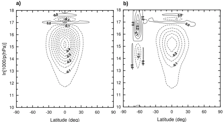
Figures 10–14 plot the UMLT distributions1hr(z,ϕ) from
Eq. (3) for the planetary waves considered.
-90 -60 -30 0 30 60 90
Latitude(deg) 10
11 12 13 14 15 16 17 18
ln
[1
000/
p(
h
P
a
)]
-90 -60 -30 0 30 60 90
Latitude (deg) 10
11 12 13 14 15 16 17 18
a)
b)
Fig. 10.Latitude-height distributions of change in heat influx in K/day due to perturbations of the CO215-µm emission during propagation of the ultra-fast Kelvin wave for 16 March(a)and 1 July(b). The dashed isolines correspond to increasing the cooling rate.
-90 -60 -30 0 30 60 90
Latitude(deg) 10
11 12 13 14 15 16 17 18
ln
[1
0
00
/p
(h
P
a
)]
-90 -60 -30 0 30 60 90
Latitude (deg) 10
11 12 13 14 15 16 17 18
a)
b)
0.001
-0.02 -0.01 0.01 0.02 0.03
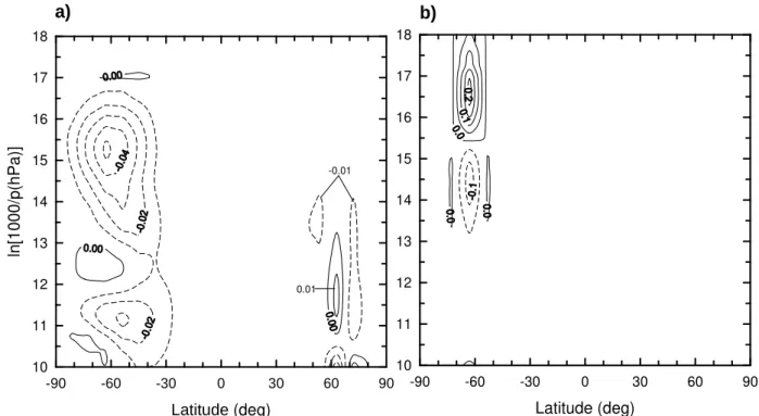
Fig. 11.As in Fig. 10, but for the 5-day wave.
cooling (1hr<0). Also similar to those estimations, the
ϕ-dependence of1hr reflects roughly that ofδT (Figs. 4–
8). Namely, the largerδT corresponds to the stronger cool-ing rate. The profilesδT(z) of the 2-, 5-, 10-, and 16-day waves in the UMLT region (Figs. 5–8) show maximums in the upper mesosphere and lower thermosphere. Those result
in maximums in the cooling rate in the 95–105 km layer of the thermosphere and near 75 km in the mesosphere. The
Table 1.Maximum order-of-magnitude of incrasing the CO215-µm band cooling rate in the upper mesosphere and lower thermosphere due to the temperature perturbations caused by a planetary wave.
Planetary Characteristic Cooling rate Cooling rate in wave (date) height (km) and in K/day Kelvin per
latitude of wave period maximum increase
in cooling rate
Ultra-fast
Kelvin wave 100, equator 0.5 3 (16 March)
2-day wave 75, 40◦N 0.02 0.5 (1 July) 100, 40◦N 0.03 0.5 5-day wave 75, 60◦S 0.001 0.005 (16 March) 100, 50◦S 0.003 0.015 10-day wave 75, 50◦S 0.05 0.5 (16 March) 100, 50◦S 0.1 1 16 day-wave 75, 50◦S 0.03 0.5 (16 March) 100, 60◦S 0.05 1
-90 -60 -30 0 30 60 90
Latitude(deg) 10
11 12 13 14 15 16 17 18
ln
[1
000/
p(
h
P
a
)]
-90 -60 -30 0 30 60 90
Latitude (deg) 10
11 12 13 14 15 16 17 18
a)
b)
Fig. 12.As in Fig. 10, but for the 10-day wave.
The maximum orders of both the rate of additional radia-tive cooling due to planetary waves and this cooling per wave period are shown in Table 1. Comparing the rate of the indi-cated “wave” cooling (Figs. 10–14) with the radiative cooling rate in the atmosphere, unperturbed by waves (Fig. 10), it is possible to conclude that the UFKW contributes maximally to all the waves to a cooling rate up to∼0.1 of the cooling rate unperturbed. In the lower thermosphere the other waves each contribute no more than∼0.01 of that. The latter asser-tion is even concerned with the 10-day wave with the
-90 -60 -30 0 30 60 90
Latitude(deg) 10
11 12 13 14 15 16 17 18
ln
[1
000/
p(
h
P
a
)]
-90 -60 -30 0 30 60 90
Latitude (deg) 10
11 12 13 14 15 16 17 18
a)
b)
-0.01
0.01
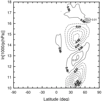
Fig. 13.As in Fig. 10, but for the 16-day wave.
Our estimates of1hr show that only the UFKW can
tan-gibly contribute to the radiative cooling of the UMLT region. The contribution of any one of the 2-, 10-, and 16-day waves does not exceed an error in estimating the radiative heat in-flux, which is certainly no less than 1%. The contribution of the 5-day wave is negligible at all.
There are T0-profiles at which heat receipts and losses compensate in fact for each other near the mesopause (see, for example, Fig. 9b), resulting in|1hr| ≥|hr,0|. At these
conditions the solar radiative heating is balanced by the ad-vection of cold and/or adiabatic cooling (Fomichev et al., 2002). The additional radiative cooling due to 2-, 5-, 10-, and 16-day waves is negligible in relation to the dynamic cooling indicated.
As is seen from Figs. 10–14, there are areas of additional heating in the CO2 15-µm band due to planetary waves (1hr>0). However, these areas are either relatively small in
volume or characterized by very small rates of heating. The “wave” heating is mainly caused by the effect of weak lines, described in Sect. 4. Their effect depends on the features of the profiles ofT0(z)andδT(z). Three cases of “wave” heat-ing are to be discussed:
1. For the 2-day wave, there is an area of heating in the upper mesosphere, centered at about 45◦N and log-pressure heightx=13 (Fig. 14). This area is configured as the area of reducedδT in Fig. 8. TheδT rise up and down from the latter area results in a sharp increase in the heat losses’ term in thehr expression. The sign of
1hr is correspondingly reversed. The case considered
shows clearly that1hr>0 can be realized only for
rela-tively little magnitudes ofδT.
2. The UFKW, 10-, and 16-day waves for 1 July and 50◦S–70◦S result in the areas of “wave” heating, which are closely configured and located in the lower thermo-sphere betweenx≈15.5 andx≈18 (Figs. 10b, 12b, and 13b). These areas coincide with the area in Fig. 9b, in which heat influx varies slightly in spite of the fact thatT0increases by a factor of∼2 in thex range indi-cated. In this case the thermospheric photon density in the CO215-µm band (see also the latter paragraph of Sect. 4) is such that a variation in thermosphericT, pro-ducing proper variations inwJ(T )and exp(−hν0/kT), does virtually not change the heat influx. The peculiar-ity in the photon denspeculiar-ity is caused by features in theT 0-profile belowx=15. The most prominent feature in the
T0-profiles under consideration is, in accordance with MSISE-90, a weak variation ofT0 with height in the range ofx≈13–15 (Fig. 2b). The case discussed is an-other example of the action of theT0-profile on 1hr.
This effect is not detected from the 2- and 5-day waves because theirδT are much weaker in the area consid-ered.
-90 -60 -30 0 30 60 90
Latitude(deg)
10 11 12 13 14 15 16 17 18
ln[
100
0/
p
(hP
a)
]
0.01
0.01
Fig. 14.As in Fig. 10, but for the 2-day wave and only for 1 July.
The distributions1hr(z,ϕ) represented only take into
ac-count theT-variation in the wave. This variation influences the radiative heat influx through theT-factor exp(−hν0/kT) of detailed balance Eq. (6), Boltzmann’s law Eq. (12) for the rotational state populations, the T-dependence of the rate constants for vibration-translation energy exchange in molecular collisions, and theT-dependence of the line shape. However, the propagation of the wave is also accompanied by the variation of air density. This variation results in an
n-variation with δn/n0∼δT/T0, where δn is the amplitude of change inn in the planetary wave, and n0 is the back-ground concentration of the air molecules. Similar to the
T-variation, the n-variation acts onhr via the coefficients
Cij, see Eqs. (4) and (5) both explicitly and implicitly. In the
latter case then-variations in a layer of the atmosphere are involved through the quantityW2, and the dependence ofhr
on those is very complicated, as is seen from Eqs. (7), (13), and (14).
It may be safe to suggest for general reasons that the wave
n-variation contributes little to 1hr as compared with the
waveT-variation. That results from the linear dependence ofCij onn, whereas the influence of theT-variation is
re-alized through nonlinear functions ofT. As was shown in our evaluations by the example of theT-variation impact, the principal influence of the wave perturbations is realized via the factors Cij in Eq. (4). However, if the averaging
overτ of the mainT-dependence in C12, specified by the factor exp(−hν0/kT), results in a tangible departure from exp(−hν0/kT0), the averaging ofngivesn0. As to the in-fluence of wave perturbations on1hr viaW2in Eq. (4), it is weak even for the T-variation. For the n-variation it is expected to be weaker.
It is seen from Eq. (13) that the rigorous consideration of
n-variation effect complicates the code for radiative transfer calculation. However, the complicating of the computational code is unlikely to be justified due to the small impact ex-pected.
6 Conclusions
1. According to the steady-state 2-D linearized model of global-scale waves, the maximum order of the wave ampli-tude of temperature in the UMLT region is equal to 15 K for UFKW, 8 K for the 10-day wave, 5 K for the 2- and 16-day waves, and 2 K for the 5-day wave.
2. The wave-caused variation in heat influx in the CO2
15-µm band, averaged over the wave period, depends on both the amplitude of temperature and the temperature profile in the atmosphere unperturbed by the wave. Although this vari-ation can be of any sign, an additional increase in radiative cooling is the prevailing effect of the planetary wave in the UMLT region. The UFKW results in an increasing of the cooling rate in the lower thermosphere up to ∼0.1 of the cooling rate in unperturbed atmosphere. The tangible con-tributions of the 2-, 10-, and 16-day waves are questionable, since their “wave” heat influxes, in accordance with our con-sideration, do not exceed an error in estimating the radiative heat influx. The contribution of the 5-day wave is negligible at all.
Acknowledgements. Our work was supported by the Russian Foun-dation for Basic Research under grant 03-05-64700 and Russian Ministry for Education under grant E02-8.0-42. V.P. Ogibalov was also partly supported by the Deutscher Akademischer Austauschdi-enst (DAAD) under grant A-03-06056 and the Wenner-Gren Foun-dation (Sweden).
Topical Editor U.-P. Hoppe thanks a referee for his help in eval-uating this paper.
References
Ahlquist, J. E.: Climatology of normal mode Rossby waves, J. At-mos. Sci., 42, 2059–2068, 1985.
Andrews, D. G., Holton, J. R., and Leovy, C. B.: Middle atmo-sphere dynamics, Academic Press, Orlando, Florida, 1987. Canziani, P. O., Holton, J. R., Fishbein, E., Froidevaux, L., and
Waters, J. W.: Equatorial Kelvin waves: A UARS MLS view, J. Atmos. Sci., 51, 3053–3076, 1994.
Dickinson, R. E.: Infrared radiative cooling in the mesosphere and lower thermosphere, J. Atmos. Terr. Phys., 46, 995–1008, 1984. Fedulina, I. N., Pogoreltsev, A. I., and Vaughan, G.: Seasonal,
inter-annual and short-term variability of planetary waves in Met Of-fice assimilated fields, Q. J. Roy. Meteorol. Soc., in press, 2004. Fomichev, V. I., Shved, G. M., and Kutepov, A. A.: Radiative cool-ing of the 30–110 km atmospheric layer, J. Atmos. Terr. Phys., 48, 529–544, 1986.
Fritts, D. C., Isler, J. R., Lieberman, R. S., Burrage, M. D., Marsh, D. R., Nakamura, T., Tsuda, T., Vincent, R. A., and Reid, I. M.: Two-day wave structure and mean flow interactions observed by radar and High Resolution Doppler Imager, J. Geophys. Res. (Sect. D), 104, 3953–3969, 1999.
Hedin, A. E.: Extension of the MSIS thermosphere model into the middle and lower atmosphere, J. Geophys. Res., A96, 1159– 1172, 1991.
Hedin, A. E., Fleming, E. L., Manson, A. H., Schmidlin, F. G., Avery, S. K., Clark, R. R., Franke, S. J., Franser, G. J., Tsuda, T., Vial, F., and Vincent, R. A.: Empirical wind model for the upper, middle and lower atmosphere, J. Atmos. Terr. Phys., 58, 1421–1447, 1996.
Khvorostovskaya, L. E., Potekhin, I. Yu., Shved, G. M., Ogibalov, V. P., and Uzyukova, T. V.: Measurement of the rate constant for quenching CO2(0110) by atomic oxygen at low temperatures: reassessment of the rate of cooling by the CO215-µm emission in the lower thermosphere, Izvestiya, Atmos. Ocean. Phys., Engl. Transl., 38, 613–624, 2002.
Kutepov, A. A. and Shved, G. M.: Radiative transfer in the 15µm CO2band with the breakdown of local thermodynamic equilib-rium in the Earth’s atmosphere, Atmos. Ocean. Phys., 14, 18–30, 1978.
Llewellyn, E. J. and McDade, I. C.: A reference model for atomic oxygen in the terrestrial atmosphere, Adv. Space Res., 18(9/10), 209–226, 1996.
Lindzen, R. S., Straus, D. M., and Katz, B.: An observational study of large-scale atmospheric Rossby waves during FGGE, J. At-mos. Sci., 41, 1320–1335, 1984.
L´opez-Puertas, M. and Taylor, F. W.: Non-LTE radiative transfer in the atmosphere, Word Scientific, Singapore, 2001.
Ogibalov, V. P., Kutepov, A. A., and Shved, G. M.: Non-local ther-modynamic equilibrium in CO2 in the middle atmosphere. II. Populations in theν1ν2mode manifold states, J. Atmos. Solar-Terr. Phys., 60, 315–329, 1998.
Ogibalov, V. P., Fomichev, V. I., and Kutepov, A. A.: Radiative heating effected by infrared CO2bands in the middle and upper atmosphere, Izvestiya, Atmos. Ocean. Phys., Engl. Transl., 36, 454–464, 2000.
Pogoreltsev, A. I.: Simulation of the influence of stationary plan-etary waves on the zonally averaged circulation of the meso-sphere/lower thermosphere region, J. Atmos. Terr. Phys., 58, 901–909, 1996.
Pogoreltsev, A. I.: Simulation of planetary waves and their influence on the zonally averaged circulation in the middle atmosphere, Earth, Planets and Space, 51, 773–784, 1999.
Pogoreltsev, A. I.: Numerical simulation of secondary planetary waves arising from the nonlinear interaction of the normal atmo-spheric modes, Phys. Chem. Earth (Part C), 26, 395–403, 2001. Roble, R. G.: Energetics of the mesosphere and thermosphere, in:
The upper mesosphere and lower thermosphere: A review of ex-periment and theory, (Ed) Johnson, R. M., and Killen, T. L., Geo-physical Monograph 87, 1–21, 1995.
Shved, G. M., Ishov, A. G., and Kutepov, A. A.: Universal func-tions for estimating total vibration-rotation band absorptance ? I. Linear molecules and spherical tops, J. Quant. Spectrosc. Radiat. Transfer, 31, 35–46, 1984.
Shved, G. M., Kutepov, A. A., and Ogibalov, V. P.: Non-local ther-modynamic equilibrium in CO2in the middle atmosphere. I. In-put data and populations of theν3mode manifold states, J. At-mos. Solar-Terr. Phys., 60, 289–314, 1998.
Smith, A. K., Preusse, P., and Oberheide, J.: Middle atmosphere Kelvin waves observed in Cryogenic Infrared Spectrometers and Telescopes for the Atmosphere (CRISTA) 1 and 2 tempera-ture and trace species, J. Geophys. Res., 107(D23), 8177, doi: 10.1029/2001JD000577, 2002.