Sensitivity of wetland methane emissions to model assumptions: application and model testing against site observations

(1)

BGD

8, 6095–6160, 2011

Sensitivity of wetland methane emissions

to model assumptions

L. Meng et al.

Title Page

Abstract Introduction

Conclusions References

Tables Figures

◭ ◮

Back Close

Full Screen / Esc

Printer-friendly Version Interactive Discussion

Discussion

P

a

per

|

Dis

cussion

P

a

per

|

Discussion

P

a

per

|

Discussio

n

P

a

per

|

Biogeosciences Discuss., 8, 6095–6160, 2011 www.biogeosciences-discuss.net/8/6095/2011/ doi:10.5194/bgd-8-6095-2011

Biogeosciences Discussions

This discussion paper is/has been under review for the journal Biogeosciences (BG). Please refer to the corresponding final paper in BG if available.

Sensitivity of wetland methane emissions

to model assumptions: application and

model testing against site observations

L. Meng1,2, P. G. M. Hess1, N. M. Mahowald2, J. B. Yavitt3, W. J. Riley4,

Z. M. Subin4, D. M. Lawrence5, S. C. Swenson5, J. Jauhiainen6, and D. R. Fuka1

1

Department of Biological and Environmental Engineering, Cornell University, Ithaca, NY 14850, USA

2

Department of Earth and Atmospheric Sciences, Cornell University, Ithaca, NY 14850, USA

3

Department of Natural Resources, Cornell University, Ithaca, NY 14850, USA

4

Earth Sciences Division, Lawrence Berkeley National Laboratory, Berkeley, CA 94720, USA

5

NCAR-CGD, P.O. Box 3000, Boulder, CO 80307, USA

6

Department of Forest Ecology, P.O. Box 27, University of Helsinki, Helsinki 00014, Finland

Received: 14 June 2011 – Accepted: 16 June 2011 – Published: 30 June 2011 Correspondence to: L. Meng (lm494@cornell.edu)

(2)

BGD

8, 6095–6160, 2011

L. Meng et al.

Title Page

Tables Figures

◭ ◮

Back Close

Full Screen / Esc

Discussion

P

a

per

|

Dis

cussion

P

a

per

|

Discussion

P

a

per

|

Discussio

n

P

a

per

|

Abstract

Methane emissions from natural wetlands and rice paddies constitute a large propor-tion of atmospheric methane, but the magnitude and year-to-year variapropor-tion of these methane sources is still unpredictable. Here we describe and evaluate the integration of a methane biogeochemical model (CLM4Me; Riley et al., 2011) into the Community

5

Land Model 4.0 (CLM4CN) in order to better explain spatial and temporal variations in methane emissions. We test new functions for soil pH and redox potential that im-pact microbial methane production in soils. We also constrain aerenchyma in plants in always-inundated areas in order to better represent wetland vegetation. Satellite

inundated fraction is explicitly prescribed in the model because there are large diff

er-10

ences between simulated fractional inundation and satellite observations. A rice paddy module is also incorporated into the model, where the fraction of land used for rice pro-duction is explicitly prescribed. The model is evaluated at the site level with vegetation cover and water table prescribed from measurements. Explicit site level evaluations

of simulated methane emissions are quite different than evaluating the grid cell

aver-15

aged emissions against available measurements. Using a baseline set of parameter values, our model-estimated average global wetland emissions for the period 1993–

2004 were 256 Tg CH4yr−

1

, and rice paddy emissions in the year 2000 were 42 Tg

CH4yr−

1

. Tropical wetlands contributed 201 Tg CH4yr−

1

, or 78 % of the global wetland

flux. Northern latitude (>50 N) systems contributed 12 Tg CH4yr−

1

. We expect this

20

latter number may be an underestimate due to the low high-latitude inundated area captured by satellites and unrealistically low high-latitude productivity and soil carbon

predicted by CLM4. Sensitivity analysis showed a large range (150–346 Tg CH4yr−

1

) in predicted global methane emissions. The large range was sensitive to: (1) the

amount of methane transported through aerenchyma, (2) soil pH (±100 Tg CH4yr−

1

),

25

and (3) redox inhibition (±45 Tg CH4yr−

1

(3)

BGD

8, 6095–6160, 2011

L. Meng et al.

Title Page

Tables Figures

◭ ◮

Back Close

Full Screen / Esc

Discussion

P

a

per

|

Dis

cussion

P

a

per

|

Discussion

P

a

per

|

Discussio

n

P

a

per

|

1 Introduction

Methane (CH4) is an important greenhouse gas and has made approximately a 12∼

15 % contribution to global warming (IPCC, 2007). Its atmospheric concentration has increased continuously since 1800 (Chappellaz et al., 1997; Etheridge et al., 1998; Rigby et al., 2008) with a relatively short period of decreases during 1999–2002

(Dlu-5

gokencky et al., 2003). Wetlands are the single largest source of atmospheric CH4,

although their estimated emissions vary from 80 to 260 Tg CH₄ annually (Matthews

and Fung, 1987; Bartlett et al., 1990; Hein et al., 1997; Walter et al., 2001; Whalen, 2005). In addition, the spatial distribution of methane emissions from wetlands is still unclear. For instance, some studies suggest that tropical regions (20 N–30 S) release

10

about 60 % of the total wetland emissions (Bartlett et al., 1990; Bartlett and Harriss, 1993), whereas other studies argue that northern wetlands contribute as much as 60 % of the total emissions (Matthews and Fung, 1987). For tropical regions, methane emis-sions are highly uncertain because (1) tropical wetlands have a large area (Matthews and Fung, 1987; Aselmann and Crutzen, 1989; Page et al., 2011) that fluctuates

sea-15

sonally and (2) methane fluxes vary significantly across different wetland types (Nahlik

and Mitsch, 2011). Rice paddies are human-made wetlands and are one of the largest anthropogenic sources of atmospheric methane. Methane emission rates from rice

paddies have been estimated to be 20 to 120 Tg CH₄yr−1 _{(Yan et al., 2009) with an}

average of 60 Tg CH₄yr−1

(Wuebbles and Hayhoe, 2002; Denman et al., 2007).

To-20

gether, rice paddies and wetlands can release 100–380 Tg CH4yr−

1

to the atmosphere. Further, recent studies identified a new source of tropical methane from non-wetland

plants that could add as much as 10–60 Tg CH₄yr−1 _{to the global budget (Keppler}

et al., 2006; Kirschbaum et al., 2006), although this source has been disputed and is still poorly quantified (Dueck et al., 2007).

25

(4)

BGD

8, 6095–6160, 2011

L. Meng et al.

Title Page

Tables Figures

◭ ◮

Back Close

Full Screen / Esc

Discussion

P

a

per

|

Dis

cussion

P

a

per

|

Discussion

P

a

per

|

Discussio

n

P

a

per

|

of wetland systems and the paucity of field and laboratory measurements to

con-strain process representations, these models used di_fferent approaches to simulate

the methane emissions. Zhuang et al. (2004) coupled a methane module to a process-based biogeochemistry model, the Terrestrial Ecosystem Model (TEM), with explicit calculation of methane production, oxidation, and transport in the soil and to the

atmo-5

sphere. Walter et al. (2001) integrated a process-based methane model with a simple hydrologic model to estimate methane emissions from wetlands with external forcing of net primary production. Cao et al. (1996) developed a methane model based on sub-strate supply by plant primary production and organic matter degradation. The most recent methane model developed by Wania et al. (2010) is fully coupled into a global

10

dynamic vegetation model designed specifically to simulate northern peatlands. This model avoids the use of some empirical relationships and parameters (such as the

Q10 temperature-dependence) used previously. As discussed above, these models

parameterize the biogeochemical processes and hydrological processes in di_fferent

ways and use different inputs (e.g., inundated area and NPP). Thus, it is not

surpris-15

ing that they produce a large range of emissions for the global methane budget. For instance, Cao et al. (1996) estimated the global methane emissions from wetlands to

be 92 Tg CH4yr−

1

while Walter et al. (2001) calculated an emission of 260 Tg CH4yr−

1

from global wetlands. This large range indicates a high degree of uncertainty in the

global methane budget. Here we attempt to understand this uncertainty and the

20

sources of this uncertainty by driving a complex process-based biogeochemical model with multiple observational constraints.

Here, and in a related article (Riley et al., 2011), we describe a process-based methane model that simulates the physical and biogeochemical processes regulat-ing terrestrial methane fluxes. Specifically, we include physical and biogeochemical

25

processes related to soil, hydrology, microbes and vegetation that account for micro-bial methane production, methane oxidation, methane and oxygen transport through

aerenchyma of wetland plants, ebullition, and methane and oxygen diffusion through

(5)

BGD

8, 6095–6160, 2011

L. Meng et al.

Title Page

Tables Figures

◭ ◮

Back Close

Full Screen / Esc

Discussion

P

a

per

|

Dis

cussion

P

a

per

|

Discussion

P

a

per

|

Discussio

n

P

a

per

|

in detail by Riley et al. (2011). Although CLM4Me can be operated as part of a fully-coupled carbon-climate-chemistry model, here we force the global methane emission model with the best available information for the current climate, including satellite de-rived inundation fraction (Prigent et al., 2007; Papa et al., 2010), rice paddy fraction (Portmann et al., 2010), soil pH, and observed meteorological forcing (Qian et al.,

5

2006). In contrast to the initial description of CLM4Me (Riley et al., 2011), we used satellite derived inundation, evaluated a new soil pH parameterization, and evaluated the predicted methane fluxes at wetland and rice paddy sites against site-level model simulations. We then extended our parameterization to the global scale and estimated the terrestrial methane flux and its sensitivities to model parameterization choices.

10

In this paper, Sect. 2 describes several new features of this model beyond those originally described in Riley et al. (2011). The data sets used to drive the model are described in Sect. 3. Model validation and comparisons with observations as well as sensitivity analysis are presented in Sect. 4. Discussion of the global methane flux is presented in Sect. 5 and conclusions are in Sect. 6.

15

2 Model descriptions and modifications

The methane biogeochemical component of CLM4 (CLM4Me) is composed of four processes: methane production, methane oxidation, methane ebullition, methane

transport through wetland plant aerenchyma, and methane diffusion through soil. In

CLM4Me, production of CH4below the water table (P mol C m−

2

s−1) is related to the

20

gridcell estimate of heterotrophic respiration from soil and litter (RH (mol C m−

2

s−1)),

soil temperature (Q′

10), pH (fpH), redox potential (fpE), and a factor accounting for the

portion of the gridcell that is seasonally inundated (S):

P=RHfCH₄Q′10SfpHfpE (1)

Here,fCH₄ is the ratio between CO2 and CH4 production which is currently set to 0.2

25

(6)

BGD

8, 6095–6160, 2011

L. Meng et al.

Title Page

Tables Figures

◭ ◮

Back Close

Full Screen / Esc

Discussion

P

a

per

|

Dis

cussion

P

a

per

|

Discussion

P

a

per

|

Discussio

n

P

a

per

|

using satellite inundation, pH, and temperature datasets. In CLM4Me,fpH and arefpE

set to 1. The pH and redox potential functions and other modifications from CLM4Me are described in detail in the following subsections, and together are referred to as

CLM4Me′.

2.1 Soil pH effects on methanogenesis

5

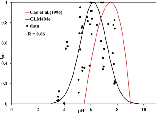
Soil pH has an important control on methane production with maximum rates at neutral pH conditions (Conrad and Schutz, 1988; Minami, 1989; Dunfield et al., 1993; Wang et al., 1993; Zhuang et al., 2004). We used the data from Dunfield et al. (1993) to

develop a new soil pH function (fpH):

fpH=10−0.2335 pH 2

+2.7727 pH−8.6 ₍₂₎

10

The maximum methane production occurs at pH∼6.2 (Fig. 1). Compared with other

functions used to specify the pH dependence of methane emissions (Cao et al., 1995; Zhuang et al., 2004) , the advantage of this new pH function is that it allows for small but finite methane production at acidic pH. Several studies have shown that methane can be produced in acidic conditions, e.g., at pH of 4.0 in northern bogs (Williams and

15

Crawford, 1985; Valentine et al., 1994). Another difference between our function and

that in Cao et al. (1995) is the optimal pH for methanogenesis, which is 7.5 in Cao et al. (1995) and 6.2 here.

2.2 Redox potential effects on methanogenesis

Methane is produced in anoxic soils only when all oxidized species such as NO−₃,

20

Fe(III), and SO2₄− are consumed because these chemical species fuel microbial

ac-tivities at the expense of methanogenesis (Lovley and Phillips, 1987). Theoretically,

methane production occurs only when redox potentials (Eh) in soil are below−200 mV

(7)

BGD

8, 6095–6160, 2011

L. Meng et al.

Title Page

Tables Figures

◭ ◮

Back Close

Full Screen / Esc

Discussion

P

a

per

|

Dis

cussion

P

a

per

|

Discussion

P

a

per

|

Discussio

n

P

a

per

|

acceptors (such as O2, NO−3, Fe

+3

, Mn4+, SO2₄−) which can suppress

methanogene-sis through the reduction of H2(Conrad, 2002) and supply more energy than available

through methanogenesis (Zehnder and Stumm, 1988). Once these alternative electron

acceptors have been depleted, H2 will increase to a level that methanogens can use

to produce methane. The duration of suppression of the alternative electron

accep-5

tors on methanogenesis will depend on their concentrations in soils and availability of

acetate and H2. The effect of redox potential has been incorporated in several

previ-ous methane models (e.g., Zhuang et al., 2004; Zhang et al., 2002; Li et al., 1999).

For instance, Zhuang et al. (2004) calculatedEh based on the status of soil

satura-tion assuming that O2 is the dominant alternative electron acceptor that suppresses

10

methanogenesis. Li et al. (1999) developed a simple dynamic model to estimate soil redox potential based on soil oxygen pressure which is calculated through soil oxygen

diffusion and consumption. In submerged soil, reducible Fe (III) is one of the most

abundant electron acceptors. Studies have suggested that methane production will not occur until a significant amount of Fe (III) has been reduced to Fe (II) (Conrad, 2002;

15

Cheng et al., 2007). Based on laboratory experiments, Cheng et al. (2007) developed an empirical model to include soil chemical properties (such as available N and Fe (II)) in predicting methane emissions from Japanese rice paddy soils. They showed that methane production is significantly related to reducible Fe and decomposable C and

found that methane production is delayed by 4–8 weeks for different types of soils due

20

to the abundance of reducible Fe. Due to the lack of globally available datasets for re-ducible Fe and other species, we do not estimate the delay time on a spatially explicit basis.

Here we developed a simple parameterization of the effects of redox potential by

assuming newly inundated wetlands will not produce methane initially because of the

25

existing electron acceptors (such as O2, SO−

2 4 , Fe

3+_{, etc) regenerated by O}

2 prior to

(8)

BGD

8, 6095–6160, 2011

L. Meng et al.

Title Page

Tables Figures

◭ ◮

Back Close

Full Screen / Esc

Discussion

P

a

per

|

Dis

cussion

P

a

per

|

Discussion

P

a

per

|

Discussio

n

P

a

per

|

of methane production. Such delayed impacts have been demonstrated in other stud-ies (Lovley and Phillips, 1987; van Bodegom and Stams, 1999; Conrad, 2002; Cheng et al., 2007). We incorporated the redox potential into CLM4Me in inundated fraction and non-inundated fractions separately.

In the inundated fraction, we modified the inundation fraction that produces methane.

5

In other words, we adjusted the fractional inundation in each grid cell to account for

changing redox potential. Therefore, the redox potential factorf_pE in Eq. (1) is

calcu-lated as follows:

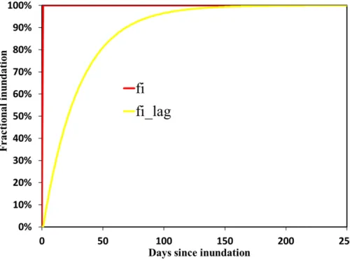
fi lag(t)=fi(t)−fredox(t) (3)

f_redox(t)=f_i(t)−fi(t−1)+fredox(t−1)·(1−∆t/τ) (4) 10

fpE=

fi lag(t)

fi(t)

(5)

wherefi(t) is the fractional inundation,fi lag(t) is the adjusted fractional inundation that

is producing methane,fredox(t) is the fraction of grid cell where alternative electron

ac-ceptors (such as O₂, NO−

3, Fe

+3

) are consumed (i.e., methane production is completely

inhibited),∆tis the time step, andτis the time constant currently set to 30 days. Thus

15

fredox(t) is equal to the newly inundated fraction of land plus a relaxation of the

previ-ously inundated fraction to zero. These are new equations that we derived based on current understanding of the impact of redox potential on methane production. Figure 2

shows the adjusted fractional inundation (fi lag) against original fractional inundation.

In the non-inundated fraction, we estimated the delay in methane production as the

20

water table depth increases by estimating an effective depth below which CH4

produc-tion can occur (Zi lag):

Zi lag(t)=Zi(t)−Zredox(t) (6)

Zredox(t)=Zi(t)−Zi(t−1)+Zredox(t−1)·(1−∆t/τ) (7)

whereZredoxis the depth of saturated water layer where alternative electron acceptors

25

(9)

BGD

8, 6095–6160, 2011

L. Meng et al.

Title Page

Tables Figures

◭ ◮

Back Close

Full Screen / Esc

Discussion

P

a

per

|

Dis

cussion

P

a

per

|

Discussion

P

a

per

|

Discussio

n

P

a

per

|

production in the unsaturated portion in each grid cell. This approach is a simplification

of the true dynamics of redox species concentrations and their impact on CH₄

pro-duction, which include vertical transport and multiple transformation processes. Future work in global-scale models should address this simplification.

2.3 Methane oxidation in the rhizosphere

5

In wetlands and rice paddies, plants develop aerenchyma to facilitate oxygen trans-port for root respiration and to suptrans-port microbial activity in the soil-root rhizosphere. However, aerenchyma can also serve as conduits for methane to escape to the atmo-sphere (Colmer, 2003). Studies suggest that aerenchyma can be a dominant pathway for plant-mediated transfer of methane from soil to the atmosphere with up to 90 %

10

of the total methane emissions via transport in the aerenchyma from the rhizosphere (Cicerone and Shetter, 1981; Nouchi et al., 1990). While the methane is escaping through aerenchyma, some of it can be oxidized by the available oxygen. Therefore, rhizospheric methane oxidation can have a large control on global methane budgets. In CLM4Me, competition of root respiration and methanotrophy for the available oxygen

15

determines the fraction of methane that is oxidized in the rhizosphere before being re-leased into the atmosphere through aerenchyma. The balance between transport and oxidation depends on the availability of oxygen in the rhizosphere (Riley et al., 2011).

The amount of O2 that can be brought to the root depends on several factors

includ-ing temperature, light intensity, water table change, and plant physiology (Whitinclud-ing and

20

Chanton, 1996; van der Nat and Middelburg, 1998). For instance, van der Nat and Mid-delburg (1998) investigated seasonal variation in rhizospheric methane oxidation of two common wetland plants (reed and bulrush) in a well-controlled environment and found that rhizospheric methane oxidation peaked during the early plant growth cycle and decreased after plants matured and root respiration decreased. We selected two sites

25

where field-measured rhizospheric oxidation fractions were measured for comparison with model predictions. A sensitivity analysis was also conducted to characterize the

(10)

BGD

8, 6095–6160, 2011

L. Meng et al.

Title Page

Tables Figures

◭ ◮

Back Close

Full Screen / Esc

Discussion

P

a

per

|

Dis

cussion

P

a

per

|

Discussion

P

a

per

|

Discussio

n

P

a

per

|

2.4 Existence of aerenchyma in mostly inundated wetlands

In this study, we assumed that plant aerenchyma develop only in plants restricted to continuously-inundated land. Although, aerenchyma represent one adaptation to

in-undation, there are other di_fferences between wetland plants and other plant types in

their ability to deal with inundation. Studies suggest that some plants in dry land do

5

not form aerenchyma (Voesenek et al., 1999), given the metabolic cost to construct and maintain tissue. Rather they adjust physiologically to seasonal flooding (Voesenek and Blom, 1989; Colmer, 2003). For instance, some cultivars of Brassica napus tend to develop new roots near the water surface in response to waterlogging (Daugherty et al., 1994; Voesenek et al., 1999). Because CLM4 does not have a wetland plant

10

functional type (pft), the methodology adapted here is designed to improve our ability to simulate soil methane dynamics without adding a new wetland pft (which in the long term is a better solution). Here we define the fraction of continuously-inundated land

(fm) as the long-term (1993–2004) mean NPP flux weighted fractional inundation (fi) at

each grid cell:

15

f_m= P

ifi·NPPi P

iNPPi

(8)

where NPP_i is the simulated average NPP at month i in the CLM4CN. To implement

this feature into the model, at each gridcell we decrease plant aerenchyma area (T)

evenly across all inundated area if current inundated fraction (f_i) is greater thanf_m as

follows:

20

T∗₌_T_·_f

aere (9)

faere=min

1,fm f_i

(10)

(11)

BGD

8, 6095–6160, 2011

L. Meng et al.

Title Page

Tables Figures

◭ ◮

Back Close

Full Screen / Esc

Discussion

P

a

per

|

Dis

cussion

P

a

per

|

Discussion

P

a

per

|

Discussio

n

P

a

per

|

increases, which agrees with other studies that show the increase of aerenchyma in wetland plants in response to flooding (Fabbri et al., 2005; Kolb and Joly, 2009). How-ever, this model feature may underestimate aerenchyma area in unflooded plants as formation of aerenchyma in some plants is not controlled by flooding conditions (Fabbri et al., 2005). This relationship only applies to natural wetlands since rice paddies are

5

assumed to always be inundated in this study.

2.5 NPP-adjusted methane flux

Uncertainties in simulated methane fluxes could possibly come from errors associated with simulated NPP. By comparing with observation-based estimate NPP, we adjusted simulated methane fluxes and evaluated how improved NPP could increase the

pre-10

dictability of methane emissions. We applied the following equation to predict simulated

methane flux (F_CH

4):

F′

CH₄=FCH4

NPPMODIS

NPP_model (11)

where F′

CH₄ is the NPP-adjusted daily methane flux (mg CH4m−

2

d−1), NPPMODIS is

the annual mean NPP derived from MODIS, and NPPmodel is the annual mean NPP

15

simulated in the CLM4CN. We applied this factor only to test the impact of substrate production uncertainty on methane emissions and not to modify our global emission estimates.

2.6 Modifications for rice paddies

In the model, the major differences between rice paddy and natural wetlands are that

20

(12)

BGD

8, 6095–6160, 2011

L. Meng et al.

Title Page

Tables Figures

◭ ◮

Back Close

Full Screen / Esc

Discussion

P

a

per

|

Dis

cussion

P

a

per

|

Discussion

P

a

per

|

Discussio

n

P

a

per

|

we used the year 2000 atmospheric forcing (Qian et al., 2006) with unlimited nitrogen to

spin-up the CLM4 model offline simulation. We also assumed only one crop pft in each

gridcell, so that the soil column would only contain rice; normally in CLM4, PFTs share a single soil column. This new spin-up is used to initialize the rice paddy simulation. In addition, only methane emissions from the inundated fraction in each gridcell are used

5

to calculate the gridcell mean emissions in the rice paddy simulations. The methane emissions from non-inundated fraction were excluded when calculating gridcell mean emissions in rice paddy module.

2.7 Model setup for point and global simulations

We compared simulated methane emissions to site level observations by running the

10

methane emission model in point simulations as well as at the global level. For point simulations, we used the atmospheric forcing data (Qian et al., 2006) from the over-lapping grid cell. Then we spun-up the model for each site by running CLM4CN as a single-point model for more than 1000 yr until the soil carbon stabilized. For these single-point simulations, we did not consider the grid-cell averaged flux for the

evalu-15

ation of our model. Instead, we calculated the methane emission fluxes from either the unsaturated or saturated portion of the grid cell depending on the local water table measurements at the site location. When the measured water table was above the surface we assumed the measured flux at the site was represented by the simulated flux in the saturated portion of the grid cell; when the measured water table is below

20

the surface we assumed the measured flux is represented by the simulated flux in the unsaturated portion of the grid cell, where the simulated water table position is taken to be the monthly water table position at the measurement location. The imposed wa-ter table level is used for the methane-related calculation of anaerobicity, production, oxidation, etc., but does not include the expected impact of water table on soil

tem-25

perature. For global wetland simulations, we used the spin-up described in Riley et al.

(2011) to initialize an o_ffline 1993–2004 run with observed meteorological forcing and

(13)

BGD

8, 6095–6160, 2011

L. Meng et al.

Title Page

Tables Figures

◭ ◮

Back Close

Full Screen / Esc

Discussion

P

a

per

|

Dis

cussion

P

a

per

|

Discussion

P

a

per

|

Discussio

n

P

a

per

|

the fraction of inundation was taken from the satellite measurements. For rice paddy

simulations, we used the spin-up described in Sect. 2.6 to initialize an o_ffline run for

year 2000.

2.8 Calculation of rhizospheric methane oxidation fraction

In order to calculate the fraction of methane oxidized in the rhizosphere, we conducted

5

two single-point simulations for each of the two sites with data on plant aerenchyma. One simulation assumed that all methane transported through aerenchyma from the rhizosphere was released into the atmosphere without loss (hereafter referred to as “NoLoss”), and the other considered methane oxidation loss in the rhizosphere before being emitted into the atmosphere (hereafter referred to as “WithLoss”). The

rhizo-10

spheric methane oxidation fraction was computed as the ratio of calculated methane

flux differences between NoLoss and WithLoss to methane flux that was transported

through aerenchyma in NoLoss. This method for calculating rhizospheric oxidation is comparable to the way it was calculated in the field experiment. In our model, we as-sumed that vegetation communities at these two sites include significant amount of

15

plants with aerenchyma.

2.9 Calculation of aerenchyma area

We also modified the Eq. (5) in Riley et al. (2011) to use fine root C instead of leaf area index in calculating aerenchyma area because fine root C calculated in CLM4-CN accounts for pft-specific and seasonal variations. This term better represents mass of

20

tiller used in Wania et al. (2010) to calculate aerenchyma area. The equation is as follows:

T=Frootc

0.22πR

2 ₍₁₂₎

whereFrootcis pft-specific fine root Carbon (g C m−

2

),R is the aerenchyma radius (2.9×

10−3

m); and the 0.22 factor represents the amount of C per tiller. We will conduct

(14)

BGD

8, 6095–6160, 2011

L. Meng et al.

Title Page

Tables Figures

◭ ◮

Back Close

Full Screen / Esc

Discussion

P

a

per

|

Dis

cussion

P

a

per

|

Discussion

P

a

per

|

Discussio

n

P

a

per

|

a sensitivity analysis to test the impact of this change on global methane budget relative to that calculated using leaf area index.

3 Datasets

We used the datasets described below to force the methane emission model to the extent possible with observed data.

5

3.1 Global distributions of wetlands and rice cultivation fields

We used satellite inundation data (1993–2004) provided by Prigent et al. (2007) and Papa et al. (2010) to represent the extent of natural wetlands and to include seasonal and interannual variability in our global simulations. As discussed in Prigent et al. (2007), the satellite inundation does not discriminate among inundated wetlands and

10

irrigated agriculture; therefore, we removed the irrigated agriculture from the satellite in-undation by assuming rice cultivation areas were inundated agricultural land. Monthly mean distributions of rice cultivation areas compiled by Portmann et al. (2010) were used to define rice location and area. Irrigated, rain-fed, and deepwater rice (Kende et al., 1998) areas are included in the rice cultivation areas. Due to the lack of

informa-15

tion on water management, draining, and re-flooding during the rice-growing season at the global scale, we assumed that rice fields were continuously flooded from the begin-ning of rice planting to the end of rice harvest. Overall, global coverage of rice paddies

totals 1.67×106km2, which is slightly larger than the areas estimated by Matthews and

Fung (1991) and Asemann and Crutzen (1989), which are 1.47×106and 1.3×106km2,

20

respectively. Rice growth areas peaked in July and August in this dataset (Fig. 3). Com-parison of satellite-derived inundated areas with wetland extents compiled from other sources shows a large deficiency (Fig. 4). On average, satellite derived inundated

areas in northern latitudes are∼37 % and∼45 % smaller than wetland extents

com-piled by Matthews and Fung (1987) (hereafter referred to as “MF”) and Aselmann and

(15)

BGD

8, 6095–6160, 2011

L. Meng et al.

Title Page

Tables Figures

◭ ◮

Back Close

Full Screen / Esc

Discussion

P

a

per

|

Dis

cussion

P

a

per

|

Discussion

P

a

per

|

Discussio

n

P

a

per

|

Crutzen (1989) (hereafter referred to as “AC”), respectively. The underestimation of the inundated area might be expected because satellites tend to underestimate small inland water bodies (inundated fraction less than 10 % of the pixels) that exist in high latitudes. Despite this weakness, the satellite-derived dataset provides a powerful tool to constrain methane emissions as it provides seasonal variations in inundated area

5

that have large impacts on the seasonal variation in methane emissions (and will be discussed below). Satellite inundated areas are 36 % and 77 % larger than MF and AC

wetland extents in temperate regions and are∼37 % and∼45 % smaller than MF and

AC wetland extents in tropical regions, respectively. As demonstrated below, the

as-sumption of wetland extent can result in large differences in simulated global methane

10

fluxes.

3.2 Global soil pH datasets

Global soil pH datasets for this study are from the global soil data set of IGBP-DIS distributed by the International Soil Reference and Information Centre (Tempel et al., 1966) (http://www.isric.org/) (Fig. 5). The original sources of these datasets are from

15

the combination of international soil reference and information center (ISRIC)’s soil information system (SIS) and CD-ROM of the Natural Resources Conservation Ser-vice (USDA-NRCS). The two datasets can be merged without issues of compatibility (Pleijsier, 1986). Note that this pH dataset does not necessarily represent wetland

con-ditions, although soil pH is thought to be an important control on wetland pH (Magdoff

20

(16)

BGD

8, 6095–6160, 2011

L. Meng et al.

Title Page

Tables Figures

◭ ◮

Back Close

Full Screen / Esc

Discussion

P

a

per

|

Dis

cussion

P

a

per

|

Discussion

P

a

per

|

Discussio

n

P

a

per

|

3.3 Observed meteorological forcing

The observed meteorological forcing dataset that is provided with CLM4 extends from

1948 to 2004 at 3-hourly temporal and T62 (∼1.875◦) spatial resolution. The dataset

is a combination of observed monthly precipitation and temperatures with model simu-lated intra-monthly variations from NCEP-NCAR 6-hourly reanalysis (Qian et al., 2006).

5

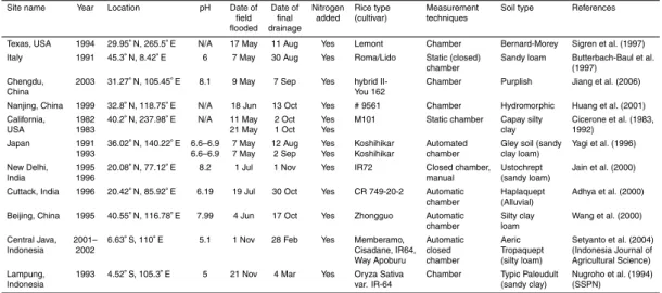
3.4 Rice paddies and wetland sites

A total of 11 rice paddy fields (Table 1) and 7 natural wetland sites (Table 2) were selected to test our model simulations. The rice paddy fields include sites in Italy, Chengdu (China), Nanjing (China), Japan, California (USA), Texas (USA), New Delhi (India), Cuttack (India), Beijing (China), Central Java (Indonesia), and Lampung

(In-10

donesia). The common feature of the selected rice growing seasons at these sites was that there was no drainage until harvest. At each location, the flooding and drainage dates were provided in their corresponding references (Table 1). The pH values were set to 6.2 (optimal pH) when not available. The soil types on paddies are mainly loam and clay. These sites were chosen to cover major rice growing regions with a focus on

15

Asia.

The wetland comparison includes sites in Panama, Indonesia, Florida, Minnesota, Michigan, Alberta (Canada), and Finland, covering the tropics, mid-latitudes, and high latitudes. Measured water table positions were integrated into the model to simulate methane emissions at these natural wetland sites (except the Panama site which used

20

modeled water table positions). We assumed that soil was inundated below the water table. These wetland sites usually have peat soils with varying depths underlain by mineral soil. Methane is produced in the wetlands from litter and dead vegetation rem-nants in anoxic conditions. For these site-level comparisons, we used NCEP-NCAR reanalysis atmospheric forcing (including precipitation, temperature, wind speeds, and

25

solar radiation) (Qian et al., 2006), pH from the site level measurement, and redox

(17)

BGD

8, 6095–6160, 2011

L. Meng et al.

Title Page

Tables Figures

◭ ◮

Back Close

Full Screen / Esc

Discussion

P

a

per

|

Dis

cussion

P

a

per

|

Discussion

P

a

per

|

Discussio

n

P

a

per

|

4 Results: model testing and sensitivity analysis

Here we discuss the comparisons of the model against site-level observations. The selected wetland sites (Table 2) have varying water table positions obtained from mea-surements (except Panama where simulated water table was used). At the northern latitude sites, water table level will not control methane emissions during winter when

5

the surface is frozen.

4.1 Net primary production (NPP)

The long-term annual mean NPP was derived from the MODerate Resolution Imaging Spectroradiometer (MODIS) and obtained from the Numerical Terradynamic Simulation Group (NTSG) (http://www.ntsg.umt.edu) (Zhao et al., 2005). At all sites, methane

10

production in the model is dependent on the model simulation of the carbon cycle. One measure of carbon uptake is net primary productivity or NPP, which is calculated by CLM4CN. Measured and simulated NPP are highly correlated, although the simulated NPP tends to overestimate observations, particularly at higher levels of NPP (Fig. 6), consistent with previous comparisons (Randerson et al., 2009).

15

4.2 Methane oxidation fraction in the rhizosphere

Simulations suggest that the model tends to overestimate the magnitude of rhizo-spheric methane oxidation fraction at the two sites with measurements (Alberta, Canada and Florida, USA) (Fig. 7). With no change in aerenchyma transport there are three ways to decrease the rhizospheric methane oxidation in the model: 1)

de-20

crease the maximum oxidation fraction (Ro,max); 2) increase the CH4 half-saturation

oxidation coefficient (KCH₄); and 3) increase the O2half-saturation oxidation coefficient

(KO₂). The values of these parameters are not well constrained and measurements

generally vary over 2 orders of magnitude (Riley et al., 2011). We found that the simulated methane flux responded similarly to the three parameters and was most

(18)

BGD

8, 6095–6160, 2011

L. Meng et al.

Title Page

Tables Figures

◭ ◮

Back Close

Full Screen / Esc

Discussion

P

a

per

|

Dis

cussion

P

a

per

|

Discussion

P

a

per

|

Discussio

n

P

a

per

|

sensitive toR_o,max. Therefore, we focused on R_o,max for our sensitivity analysis. We

decreasedR_o,maxfrom 1.25×10−5 to 1.25×10−6, still within the estimated parameter

uncertainty given in Riley et al. (2011), which led to a closer match of simulated rhi-zospheric methane oxidation fraction with observations (Fig. 7). We then tested the

sensitivity of global methane budget to this parameter and applied this lowerRo,max to

5

the global simulation. The model estimated a 12 % increase in global methane fluxes

using the lowerRo,max(Table 7). We also note that there is a spring peak in methane

emission at Alberta (Canada) and Michigan (USA) sites in Fig. 7. A detailed description of this phenomenon is provided in Appendix B (Fig. B).

4.3 Impacts of pH on methane emission

10

There are three sites that have pH values more acidic than neutral conditions, allowing us to test our pH function against observed methane fluxes. In each case the site level pH is obtained from local measurements.

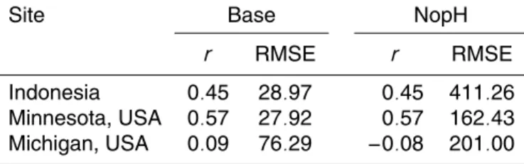
Soil pH plays an important role in constraining model simulations to the observa-tions at several sites where soils are acidic (Fig. 8, Table 2). For example, at the

In-15

donesian site, if we remove the pH impact, the model simulated methane emissions of

>300 mg CH₄m−2_d−1_{which is}_>_{30 to 80 times larger than the measurements}

(approx-imately 10 mg CH₄m−2

d−1

). Soil pH is also an important control on methane emissions at Minnesota and Michigan sites. Removal of the pH factor at these sites increases the methane emissions by a factor of 4–5. Including the pH factor allows for better

agree-20

ment with observations (Fig. 8). Table 3 shows thatfpH has reduced the RMSE at all

sites, although, fpH has negligible impacts on the ability to simulate the seasonal

cy-cle (seen in the correlation coefficient) (Table 3). These results suggest that pH is an

important control on regional methane budgets, and should be included in models to produce accurate spatial distribution and magnitudes of methane emission. A scatter

25

(19)

BGD

8, 6095–6160, 2011

L. Meng et al.

Title Page

Tables Figures

◭ ◮

Back Close

Full Screen / Esc

Discussion

P

a

per

|

Dis

cussion

P

a

per

|

Discussion

P

a

per

|

Discussio

n

P

a

per

|

4.4 Impact of redox potential on methane emissions

Our simulations suggest that redox potential does not have substantial impacts on methane emissions at the sites where we have observations of water table levels (not shown). This low sensitivity is because of the relatively small changes in water table fluctuation at these sites (for detailed information see the description of each site given

5

in the Table 2 references). At each individual site, the impact of redox potential on methane production is predominately through the change in water table levels. This

dependence is different from the large-scale simulation where the impact of redox

po-tential is largely seen through changes in the inundated fraction. In the large-scale simulation, the impact of redox potential in the unsaturated zone is through the change

10

in water table levels and is negligible since very little methane is produced and re-leased into the atmosphere. The redox potential factor does play an important role in large-scale methane emissions when the inundated fraction dramatically changes from season to season. Figure 9 shows the impact of redox potential on methane emission at a gridcell near Michigan extracted from a global CLM4 simulation. These

simula-15

tions suggest that modeled methane emissions are reduced due to the fact that the

inundated fraction that produces methane (fi lag, red dashed line) is much lower than

the actual inundated fraction (fi, blue dashed line). We want to emphasize that this

pro-posed mechanism has not been tested against observations but matches theoretical expectations.

20

4.5 Site simulations: rice paddies

We simulated the rice paddies as single-gridcell cases and assumed that the fields were submerged during the simulation period between initial flooding and final

drainage. In general, CLM4Me′as modified for rice paddies captures the magnitudes

and temporal variations of methane emissions during the growing season (Fig. 10).

25

(20)

BGD

8, 6095–6160, 2011

L. Meng et al.

Title Page

Tables Figures

◭ ◮

Back Close

Full Screen / Esc

Discussion

P

a

per

|

Dis

cussion

P

a

per

|

Discussion

P

a

per

|

Discussio

n

P

a

per

|

California and Japan (Fig. 10d–f), but not at the other sites, possibly due to the duration and frequency of measurements (i.e., once a week). The sudden increase in simu-lated methane emissions immediately after drainage can be attributed to the release of methane previously trapped in the soil and water. This flush of methane has also been demonstrated in other studies (Wassmann et al., 1994; Jain et al., 2000). On a

growing-5

season mean basis, the model performed relatively well for sites with observed mean

fluxes less than 200 mg CH₄m−2d−1, and less well for sites with greater than a mean of

200 mg CH₄m−2_d−1_{(Fig. 11a). Simulated maximum CH}

4emissions matched

observa-tions relatively well for sites with maximum daily fluxes less than 300 mg CH4m−

2

d−1,

but less well for sites with values greater than about 300 mg CH4m−

2

d−1 (Fig. 11b).

10

For the latter sites, the model has a low bias.

4.6 NPP-adjusted methane fluxes

Scatter plots show that the NPP-based adjustment to simulated methane emissions only slightly increased the correlation with the measurements and did not improve the RMSE (Fig. 11). For instance, the correlation between modeled and observed mean

15

fluxes increased from 0.5 to 0.61 using the NPP-based adjustment, primarily due to the adjustment at the Panama site (Fig. 11a). Overall, adjusting for NPP did not sig-nificantly improve model simulations at all other sites. This result suggests that the methane emission model biases are not just because of errors in the NPP.

4.7 Global simulations vs. observations

20

We note that our global simulations were forced with satellite inundation data and the same NCEP forcing data as used for the site simulations. To compare the global sim-ulation against site level measurements, we extracted methane fluxes from the satu-rated portion of the closest grid cells to both the natural wetlands and rice paddies in the global simulation and compared with site level observations. This is the best

25

(21)

BGD

8, 6095–6160, 2011

L. Meng et al.

Title Page

Tables Figures

◭ ◮

Back Close

Full Screen / Esc

Discussion

P

a

per

|

Dis

cussion

P

a

per

|

Discussion

P

a

per

|

Discussio

n

P

a

per

|

thus a commonly used approach. We used methane fluxes from the saturated portion because they are very close to site-level conditions where the water table level is close to the surface, as is the case at most of the sites.

Comparison between mean methane fluxes in the global simulation and observations

at sites shows a poor correlation (r=0.2) (Fig. 12). Comparing with Fig. 11 suggests

5

that the model’s performance is worse in simulating the magnitude of methane fluxes when comparing grid-cell methane fluxes obtained from global simulations with point

measurements. For instance, the correlation (r) decreased and the RMSE increased

in Fig. 12. This result is not unexpected because of spatial heterogeneity and the large

spatial resolution (1.9◦×2.5◦ resolution) used in the global simulation. We suggest

10

that model should be validated at the site level if localized information is available, ideally forced by local vegetation characteristics, water table depth, and near-surface meteorology.

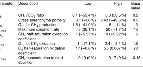
4.8 Sensitivity analysis at individual sites

Seven parameters were selected for sensitivity analysis (Table 4). The value for each

15

parameter was varied from the lower end to the higher end of its range in the references listed in Table 4 to test its impacts on modeled methane emissions. The Panama site was selected for this analysis. The percentage change in annually averaged methane emission rate relative to the base simulation is listed in parenthesis in Table 5 for each

parameter. TheQ10 for production, fCH₄, and the porosity of tillers have the most

sig-20

nificant impacts on simulated methane emissions at this site. This result is consistent with the sensitivity analysis conducted by Wania et al. (2010) and Riley et al. (2011).

The maximum oxidation rate (R_o,max) has a moderate impact on methane emissions.

Other parameters, includingKCH₄,Qo,10,Ko2, andCe,max, have smallest influences on

methane emissions. For instance, varyingCe,maxvalues within the range of current

es-25

timates negligibly affects methane emissions. Sensitivity analysis conducted at several

(22)

BGD

8, 6095–6160, 2011

L. Meng et al.

Title Page

Tables Figures

◭ ◮

Back Close

Full Screen / Esc

Discussion

P

a

per

|

Dis

cussion

P

a

per

|

Discussion

P

a

per

|

Discussio

n

P

a

per

|

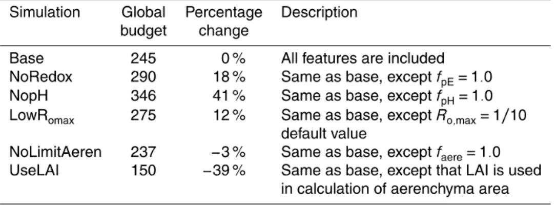
4.9 Sensitivity analysis on the global methane budget from natural wetlands

In this section, we focused our analysis on wetland emissions. For this sensitivity analysis, we conducted two year (1992–1993) simulations and used the second year for this analysis. We conducted the sensitivity analysis with the following parameters:

soil pH (fpH), redox potential (fpE), and the limitation on aerenchyma area (faere). The

5

processes these parameter impact have very different impacts on the global methane

budget. We note that uncertainties in model structure and other model parameters listed in Table 4 could also have significant impacts on global emissions. These uncer-tainties have been discussed in Riley et al. (2011) and are not included in this paper.

In general, the inclusion of soil pH (fpH) and redox potential (fpE) decreased methane

10

emissions. The limitation on aerenchyma area (faere) decreased methane oxidation,

causing an increase in methane emissions. Model results suggest that the impacts of these factors on the global and regional methane budget vary (Fig. 13). Soil pH has the largest impacts on methane emissions. On the global scale, exclusion of soil pH

in methane production (fpH=1.0) increased methane emissions by 100 Tg CH4yr−

1

,

15

an approximate 41 % increase from the base simulation (Table 7). Removal of redox

potential impacts (fpE=1.0) increases global methane emissions to 290 Tg CH4yr−

1

(a 18 % increase from the base simulation). Unlimited aerenchyma (faere=1.0) only

decreased the global methane budget by 3 %. At the regional scales, approximately 70 % of the global impacts of these factors occurred in the tropics (Fig. 13a), as

trop-20

ical regions account for 80 % of the global methane wetland emissions and soil pH is generally low there (Fig. 5).

Our simulations suggest that the rhizospheric methane oxidation fraction is generally higher in temperate regions and lower in the tropics and high latitudes (Fig. 13b). The rhizospheric oxidation fraction is approximately 11.4 %, 25.4 %, and 23 % in the tropics,

25

temperate, and high latitudes, respectively. On the global scale,∼15 % of methane was

(23)

BGD

8, 6095–6160, 2011

L. Meng et al.

Title Page

Tables Figures

◭ ◮

Back Close

Full Screen / Esc

Discussion

P

a

per

|

Dis

cussion

P

a

per

|

Discussion

P

a

per

|

Discussio

n

P

a

per

|

also develop conduits (Grosse et al., 1992). The default value for aerenchyma in trees is set to be 17 % of that in grasses. Adjusting this proportion from 1 % to 35 % changed

the methane flux by less than 25 Tg CH4yr−

1

(<10 % of global methane budget).

4.10 Fine root carbon (FROOTC) vs. leaf area index (LAI)

Our modeling results suggest that simulated global methane budget is very sensitive to

5

the way the aerenchyma area is calculated (Table 7). When the aerenchyma area was calculated based on FROOTC using Eq. (11) in this paper, the model’s methane

emis-sions are 245 Tg yr−1_{. When LAI is used to calculate aerenchyma area, the methane}

emissions were 150 Tg yr−1, an approximately 39 % decrease relative to FROOTC

method.

10

5 Estimation of global methane flux

5.1 Global simulations-wetlands

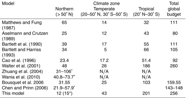
We estimated global wetland methane emissions of 256 Tg CH₄yr−1_{, which is close to}

the estimate of Walter et al. (2001), but higher than other estimates (Aselmann and Crutzen, 1989; Bartlett et al., 1990; Fung et al., 1991; Bartlett and Harriss, 1993)

15

(Table 6). Figure 14 shows the spatial distribution of mean methane flux for the period 1993–2004 from natural wetlands. A comparison of the global methane emissions

between CLM4Me′ and other models is compared in Fig. 15 (Matthews and Fung,

1987; Aselmann and Crutzen, 1989; Bartlett et al., 1990; Bartlett and Harriss, 1993; Cao et al., 1996; Walter et al., 2001; Bousquet et al., 2006; Riley et al., 2011). The

20

CLM4Me′estimate is at the low end of current estimates for high latitude wetlands and

at the high end for tropical and temperate wetlands.

Tropical wetlands released 201 Tg CH4yr−

1

(24)

BGD

8, 6095–6160, 2011

L. Meng et al.

Title Page

Tables Figures

◭ ◮

Back Close

Full Screen / Esc

Discussion

P

a

per

|

Dis

cussion

P

a

per

|

Discussion

P

a

per

|

Discussio

n

P

a

per

|

Bartlett and Harriss (1993) who calculated global wetland CH₄ emissions using

avail-able methane flux measurements and the wetland areas compiled by MF and AC. This high proportion occurs even though mean satellite inundated areas in the tropics are 31 % and 39 % lower than the MF and AC wetland extents, indicating that the methane

productivity in CLM4Me′is larger or oxidation is lower than other models. Higher

trop-5

ical production may be partially attributed to the fact that CLMCN overestimates gross primary production over the tropical regions (Bonan et al., 2011). It is also demon-strated in the Panama site (one of the tropical sites) where accurate NPP could im-prove model estimation against observation (Fig. 11a). For middle-latitude regions, the

CLM4Me′ estimate is approximately 2 times larger than other process-based models

10

(model 1–6 on Fig. 15) partially because satellite inundated areas are 48 % and 92 % larger than the MF and AC wetland extents used in other models.

CLM4Me′high latitude (>50◦N) wetlands released∼12 Tg CH4yr−

1

, which is much lower than other estimates. One of the primary reasons for the low high-latitude emis-sions could be that we assume a smaller inundation in the high latitudes, compared to

15

other estimates (Fig. 4). Another reason is that CLM4CN under-predicts high latitude vegetation productivity and soil carbon storage (Lawrence et al., 2011). There is still considerable uncertainty in the wetland extent in the high latitudes (Finlayson et al., 1999; Papa et al., 2010), and the satellite inundated area we use may not capture all of the relevant wetland area (Prigent et al., 2007). Reducing the uncertainty associated

20

with wetland extent might help further improve the estimation of the methane flux. For

pan-arctic regions (North of 45◦N), CLM4Me′ estimated 15 Tg CH4yr−

1

were released into the atmosphere. This value is lower than the estimates using various

process-based models (31–106 Tg CH4yr−

1

) (Cao et al., 1996; Walter et al., 2001; Zhuang et al., 2004; Wania et al., 2010) (Table 6), but is close to the estimate of Chen and

25

Prinn (2006) in an inverse calculation. Wania et al. (2010) calculated an emission of

21.9–57.9 Tg CH4yr−

1

from northern wetlands in Chen and Prinn’s inverse model

re-sults assuming a methane uptake of 6.9 Tg CH4yr−

1

(25)

BGD

8, 6095–6160, 2011

L. Meng et al.

Title Page

Tables Figures

◭ ◮

Back Close

Full Screen / Esc

Discussion

P

a

per

|

Dis

cussion

P

a

per

|

Discussion

P

a

per

|

Discussio

n

P

a

per

|

Seasonal variations of methane emissions in the tropics, temperate climatic zones, and northern latitudes generally follow the pattern of the inundated areas measured by satellite (Fig. 14a,b). This relationship occurs because satellite inundated areas were used to derive methane emissions in each gridcell. As can be seen in Fig. 14a,

sea-sonal variations between south and north of the equator have a different seasonality.

5

Peak methane emissions occur in the rainy season, which is generally from June to Oc-tober to the north of the equator and from OcOc-tober to March to the south of the equator. The seasonality of methane emissions in our model agrees well with that estimated in Cao et al. (1996) (their Fig. 3).

Even though our model simulated a low methane emission rate from northern

lati-10

tudes (>50◦_{N) in the summer, the seasonality of the satellite inundated areas is}

pro-nounced with maximum inundation in summer (Fig. 14b). The high inundated area in northern latitudes indicates that this region could potentially be a source of atmo-spheric methane that grows in importance because the duration and magnitude of methane production could increase as it experiences warming.

15

5.2 Global simulation of rice paddies

On average, our model estimates that global rice paddies emit approximately 42 Tg CH₄yr−1

into the atmosphere, assuming no mid-season drainage. Our estimate

is in the middle of current estimates of 26–120 Tg CH4yr−

1

(Fig. 13c) (Seiler et al., 1984; Holzapfelpschorn and Seiler, 1986; Bouwman, 1990; Sass, 1994; Cao et al.,

20

1995, 1998; Scheehle et al., 2002; Wuebbles and Hayhoe, 2002; Olivier et al., 2005; Chen and Prinn, 2006; Yan et al., 2009). For instance, Cao et al. (1998) estimated

global emissions from rice paddies to be ∼53 Tg CH4yr−

1

using MF rice paddy

ar-eas. On the regional scale, CLM4Me′ predicts 39 Tg CH₄yr−1 is released from rice

paddies in the Asian monsoon region (10◦_S–50◦_{N, 65}◦_E–145◦_{E) which contributes}

25

(26)

BGD

8, 6095–6160, 2011

L. Meng et al.

Title Page

Tables Figures

◭ ◮

Back Close

Full Screen / Esc

Discussion

P

a

per

|

Dis

cussion

P

a

per

|

Discussion

P

a

per

|

Discussio

n

P

a

per

|

forced with fractional rice cover compiled by Leff et al. (2004) (Spahni et al., 2011).

Chinese rice paddies release more CH4 than any other country. In our model,

Chi-nese rice paddies released∼10 Tg CH4yr−

1

, which is in the middle of other estimates

(7∼17 Tg CH4yr−

1

) derived using agricultural activity data and field measurements (Matthews et al., 2000; Li et al., 2004; Yan et al., 2009; Kai et al., 2010). For instance,

5

Yan et al. (2009) estimated the methane emissions from Chinese rice paddies to be

7.41 Tg CH4yr−

1

using the IPCC 2006 guidelines for national greenhouse gas invento-ries and methane emissions from rice paddies, and agricultural activity data for 2000.

Yan et al. (2003) estimated emissions of 7.67 Tg CH4yr−

1

in 1995 for China using

mea-surements and region-specific CH4emission factors. Recently, Kai et al. (2010) revised

10

the Huang model to include the effect of fertilizer use and water management and found

that methane emissions from Chinese rice fields peaked in 1982 with an emission of

∼11 Tg CH4yr−

1

in 2000. This estimate agrees with our estimates very well since we used the rice paddy fraction dataset developed by Portmann et al. (2010) for the year 2000.

15

Our model may overestimate methane emission from rice paddies for several

rea-sons. First, we assumed continuous flooding during the growing season.

Previ-ous studies have suggested that mid-season drainages have been critical to reduce methane emissions in rice paddy fields. For instance, Yan et al. (2009) showed that one-time drainage in continuously flooded fields will reduce methane emissions by

20

4.1 Tg CH₄yr−1

globally. Wassmann et al. (2000) suggested that mid-season drainage could reduce associated methane emissions by 7–80 %. On average only about 30– 40 % of rice paddies experience continuous flooding (Yan et al., 2009). Simulation with one time drainage in August in our model (not shown) decreased methane emissions

by 6 Tg CH4yr−

1

globally, or by about 14 % of the total methane emissions from rice

25