SHIMMER (1.0): a novel mathematical model for microbial and biogeochemical dynamics in glacier forefield ecosystems

(1)

GMDD

8, 6143–6216, 2015

SHIMMER (1.0): a novel mathematical

model

J. A. Bradley et al.

Title Page

Abstract Introduction

Conclusions References

Tables Figures

◭ ◮

Back Close

Full Screen / Esc

Printer-friendly Version

Interactive Discussion

Discussion

P

a

per

|

Discussion

P

a

per

|

Discussion

P

a

per

|

Discussion

P

a

per

|

Geosci. Model Dev. Discuss., 8, 6143–6216, 2015 www.geosci-model-dev-discuss.net/8/6143/2015/ doi:10.5194/gmdd-8-6143-2015

This discussion paper is/has been under review for the journal Geoscientific Model Development (GMD). Please refer to the corresponding final paper in GMD if available.

SHIMMER (1.0): a novel mathematical

model for microbial and biogeochemical

dynamics in glacier forefield ecosystems

J. A. Bradley1,2, A. M. Anesio1, J. S. Singarayer3, M. R. Heath4, and S. Arndt2

1

Bristol Glaciology Centre, School of Geographical Sciences, University of Bristol, Bristol, BS8 1SS, UK

2

BRIDGE, School of Geographical Sciences, University of Bristol, Bristol, BS8 1SS, UK

3

Department of Meteorology, University of Reading, Reading, RG6 6BB, UK

4

Department of Mathematics and Statistics, University of Strathclyde, Glasgow, G1 1XH, UK

Received: 9 July 2015 – Accepted: 15 July 2015 – Published: 6 August 2015

Correspondence to: J. A. Bradley ([email protected])

(2)

GMDD

8, 6143–6216, 2015

model

Title Page

Tables Figures

◭ ◮

Back Close

Full Screen / Esc

Discussion

P

a

per

|

Discussion

P

a

per

|

Discussion

P

a

per

|

Discussion

P

a

per

|

Abstract

SHIMMER (Soil biogeocHemIcal Model for Microbial Ecosystem Response) is a new numerical modelling framework which is developed as part of an interdisciplinary, itera-tive, model-data based approach fully integrating fieldwork and laboratory experiments with model development, testing, and application. SHIMMER is designed to simulate

5

the establishment of microbial biomass and associated biogeochemical cycling during the initial stages of ecosystem development in glacier forefield soils. However, it is also transferable to other extreme ecosystem types (such as desert soils or the surface of glaciers). The model mechanistically describes and predicts transformations in carbon, nitrogen and phosphorus through aggregated components of the microbial community

10

as a set of coupled ordinary di_fferential equations. The rationale for development of the model arises from decades of empirical observation on the initial stages of soil devel-opment in glacier forefields. SHIMMER enables a quantitative and process focussed approach to synthesising the existing empirical data and advancing understanding of microbial and biogeochemical dynamics. Here, we provide a detailed description of

15

SHIMMER. The performance of SHIMMER is then tested in two case studies using published data from the Damma Glacier forefield in Switzerland and the Athabasca Glacier in Canada. In addition, a sensitivity analysis helps identify the most sensitive and unconstrained model parameters. Results show that the accumulation of microbial biomass is highly dependent on variation in microbial growth and death rate constants,

20

Q₁₀ values, the active fraction of microbial biomass, and the reactivity of organic mat-ter. The model correctly predicts the rapid accumulation of microbial biomass observed during the initial stages of succession in the forefields of both the case study systems. Simulation results indicate that primary production is responsible for the initial build-up of substrate that subsequently supports heterotrophic growth. However, allochthonous

25

(3)

respon-GMDD

8, 6143–6216, 2015

model

Title Page

Tables Figures

◭ ◮

Back Close

Full Screen / Esc

Discussion

P

a

per

|

Discussion

P

a

per

|

Discussion

P

a

per

|

Discussion

P

a

per

|

sible for the initial accumulation of available nitrates in the soil. Biogeochemical rates are highly seasonal, as observed in experimental data. The development and appli-cation of SHIMMER not only provides important new insights into forefield dynamics, but also highlights aspects of these systems that require further field and laboratory research. The most pressing advances need to come in quantifying nutrient budgets

5

and biogeochemical rates, in exploring seasonality, the fate of allochthonous deposition in relation to autochthonous production, and empirical studies of microbial growth and cell death, to increase understanding of how glacier forefield development contributes to the global biogeochemical cycling and climate in the future.

1 Introduction

10

Ice fronts in polar and alpine regions are retreating as a result of climate warming, and as a consequence, glacier forefield areas in high latitude and high altitude regions are rapidly expanding (Graversen et al., 2008; ACIA, 2005). Glacier coverage in upland Alpine regions in Europe have declined by up to 30 % from the 1970s to 2003, expos-ing roughly 860 km2 of previously ice-covered land area (Paul et al., 2011). Similarly,

15

rapid glacial retreat has been observed in Iceland (Staines et al., 2014), North America (Insam and Haselwandter, 1989; Hahn and Quideau, 2013; Ohtonen et al., 1999; Sat-tin et al., 2009), Asia (Liu et al., 2012) and Svalbard (Moreau et al., 2008). These vast expanses of newly uncovered land have been locked under ice for tens of thousands of years, are typically highly oligotrophic, with low nutrient budgets and are subject to

20

harsh and rapidly fluctuating environmental conditions. They have potentially signifi-cant yet largely unexplored roles on large scale biogeochemical cycling and climate (Dessert et al., 2003; Anderson et al., 2000; Smittenberg et al., 2012; Berner et al., 1983), global methane budgets (Kirschke et al., 2013), the global phosphorus cycle (Filippelli, 2002; Follmi et al., 2009) and the productivity of downstream and coastal

25

(4)

GMDD

8, 6143–6216, 2015

model

Title Page

Tables Figures

◭ ◮

Back Close

Full Screen / Esc

Discussion

P

a

per

|

Discussion

P

a

per

|

Discussion

P

a

per

|

Discussion

P

a

per

|

soils is fundamental to understanding life in extreme environments, which may serve as an analogue for survival and habitability of environments currently assumed devoid of life on this planet and others.

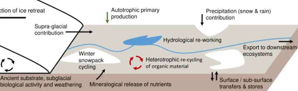
Microbial communities are the primary colonisers of recently exposed soils, and are thought to be fundamental in soil stabilisation, the build-up of carbon and nutrient pools,

5

creating a favourable habitat and facilitating the establishment of higher order plants (Schulz et al., 2013; Bradley et al., 2014). A conceptual overview of forefield nutrient cycling is presented in Fig. 1. Recently de-glaciated soils vary in their mineralogical and microbial compositions. Total Organic Carbon (TOC), Total Nitrogen (TN), and To-tal Phosphorus (TP) content of newly exposed glacial forefield soils is low, in the range

10

of 0.1–40.0 mg C g−1, 0.1–2.0 mg N g−1, and 2–8 µg P g−1 (Bradley et al., 2014). How-ever, these typically increase by 1 to 2 orders of magnitude with ageing from newly exposed to well-developed (decades old) soil. Three distinct sources contribute carbon to recently exposed soils: autochthonous primary production by autotrophic microor-ganisms, allochthonous material deposited on the soil surface (from wind, hydrology,

15

biology and precipitation) and ancient organic pools derived from under the glacier. Organic matter accumulation from all three sources supports the development of het-erotrophic communities, yet their relative significance remains unknown. The continual autotrophic production, heterotrophic re-working and allochthonous deposition lead to the accumulation of organic material, which supports higher abundances and

diver-20

sity of microorganisms (Bradley et al., 2014; Schulz et al., 2013). Nitrogen is derived from active nitrogen-fixing organisms, allochthonous deposition, and degradation of or-ganic substrate. Bioavailable phosphorus is usually abundant in the topsoil or bedrock of glaciated regions from weathering of the mineral surface, and can also be liberated due to the degradation of organic molecules.

25

(5)

GMDD

8, 6143–6216, 2015

model

Title Page

Tables Figures

◭ ◮

Back Close

Full Screen / Esc

Discussion

P

a

per

|

Discussion

P

a

per

|

Discussion

P

a

per

|

Discussion

P

a

per

|

contribution to global nutrient pathways and our ability to predict how these rapidly expanding ecosystems may respond in the future, including their potential impact on atmospheric CO₂, global climate, and downstream productivity.

This lack of understanding can be partly attributed to the difficulty of quantifying the different external organic matter and nutrient fluxes, as well as disentangling the

5

complexity of biogeochemical processes underlying the microbial dynamics and soil carbon and nutrient build-up along the chronosequence by observations and/or lab-oratory experiments alone. Numerical models are useful tools in this context as they can not only help to disentangle the complex process interplay, diagnose the fluxes be-tween ecosystem components and, ultimately, predict the sensitivity and response of

10

an environment to changing environmental and climatic conditions, but can also help identify important data and knowledge gaps and hence guide the design of e_fficient field campaigns and laboratory studies directly targeted at closing these gaps. Never-theless, a modelling framework that could be used to explore microbial dynamics and associated nutrient cycling in glacier forefields currently does not exist.

15

The development of soil models has been common in the past and important in informing soil management, policy and prediction (McGill, 2007, 1996), for example in understanding the contribution of Soil Organic Matter (SOM) to the formation of stable aggregate soils, the ease of soil cultivation, water holding characteristics, and the decreased risk of physical damage and compaction. The explicit inclusion of soil

20

microbial dynamics has been shown to drastically improve the performance of these models (Wieder et al., 2013). There are many di_fferent types of soil models in use today across a range of scales and purposes, such as informing agricultural policy, understanding biogeochemical cycling and soil food webs, and the feedbacks between soil processes, hydrology and the atmosphere (Stapleton et al., 2005; Blagodatsky and

25

(6)

GMDD

8, 6143–6216, 2015

model

Title Page

Tables Figures

◭ ◮

Back Close

Full Screen / Esc

Discussion

P

a

per

|

Discussion

P

a

per

|

Discussion

P

a

per

|

Discussion

P

a

per

|

Moorhead and Sinsabaugh, 2006; Panikov and Sizova, 1996; Toal et al., 2000; Zelenev et al., 2000; Scott et al., 1995). However, although these models include an explicit microbial component, SOM models are tailored towards research questions that are focused on geochemistry and specifically organic matter dynamics rather than biology. The models presented in the literature quickly become complex and thus require

5

comprehensive data sets for set-up, calibration and evaluation. Many of their param-eters cannot be constrained on the basis of information available for glacier forefield ecosystems, thus resulting in large uncertainties, making subsequent analysis di_ffi -cult and results sometimes unclear (Hellweger and Bucci, 2009; Beven and Binley, 1992). Accordingly, their model structure is not suitable for the study of glacial

fore-10

fields. Unique nutrient cycles, extreme and highly variable environmental conditions and rapidly changing compositions of microbial communities interact to form chronose-quence dynamics often seen only in forefield ecosystems (Bradley et al., 2014). There is not a single model that incorporates all of the necessary conditions to model fore-field development without an unacceptable level of abstraction and simplification of the

15

system.

Therefore, we developed the new model framework SHIMMER (Soil biogeocHemIcal Model for Microbial Ecosystem Response) to quantitatively simulate the initial stages of ecosystem development and assess biogeochemical processes in the forefield of glaciers. The code is written and executed in the free open source computing

envi-20

ronment and programming language R, which is available to download on the web (http://www.r-project.org/). SHIMMER is not only a new model framework, but is also part of an interdisciplinary, iterative, open-source, model-data based approach fully in-tegrating fieldwork and laboratory experiments with model development, testing, and application. More specifically, the model scope and complexity of the first version of

25

(7)

GMDD

8, 6143–6216, 2015

model

Title Page

Tables Figures

◭ ◮

Back Close

Full Screen / Esc

Discussion

P

a

per

|

Discussion

P

a

per

|

Discussion

P

a

per

|

Discussion

P

a

per

|

of a retreating Svalbard glacier. The model framework is aimed at identifying the dom-inant processes and biogeochemical controls on glaciated forefield ecosystem de-velopment. The model is kept as general as possible, thus is easily transferable to other microbial ecosystems such as desert soils or glacier surfaces. Simplifications are made to account for the quality and availability of observational data and processes

5

will be resolved at greater detail once suitable data becomes available. However, the model is dynamically sufficient, i.e. the minimum processes that are needed to re-solve the system and provide useful output are included. Some additional processes are included such as the ability of soil microbes to fix atmospheric nitrogen or assimi-late nitrate depending on soil Dissolved Inorganic Nitrogen (DIN) levels, allochthonous

10

substrate and nutrient inputs, varying levels of substrate bioavailability, and the micro-bial response to daily and seasonally varying environmental fluctuations. An important feature of the first version of the SHIMMER model is the inclusion of multiple pools of microbial biomass, each with certain functions and characteristics, to represent the diversity of species commonly found in a glacier forefield (Bradley et al., 2014). The

15

current version of the model is designed to represent the microbial community prior to the establishment of plants, and therefore only the initial stages of chronosequence development will be assessed. Microbial communities may be heavily structured by establishing vegetation (Brown and Jumpponen, 2014), and the physical properties of vegetated soils are considerably di_fferent in terms of water retention, ultra-violet

ex-20

posure, temperature fluctuations (Ensign et al., 2006; King et al., 2008), and nutrient status (Kastovska et al., 2005; Schutte et al., 2009).

This paper provides a comprehensive description of the modelling framework. The newly developed model presented here is then used to conduct an extensive parameter sensitivity study. In addition, a first model performance test is conducted on the basis

25

(8)

in-GMDD

8, 6143–6216, 2015

model

Title Page

Tables Figures

◭ ◮

Back Close

Full Screen / Esc

Discussion

P

a

per

|

Discussion

P

a

per

|

Discussion

P

a

per

|

Discussion

P

a

per

|

form a series of future laboratory experiments that will help constrain the most sensitive and/or unconstrained model parameters for our study site. Furthermore, the sensitiv-ity study and the test case studies will inform the design of additional fieldwork that will help further quantify important processes and model forcings. It is expected that the model scope and complexity will increase as more field data becomes available.

5

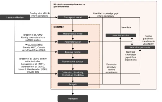
In addition, it is intended that new model developments will guide and inform future field and laboratory studies so that subsequent versions of the model will run with nar-rower plausible ranges of parameters, and explicitly resolve processes that currently cannot be constrained on the basis of available data. SHIMMER can thus be consid-ered as the first step of an interdisciplinary, iterative approach (illustrated in Fig. 2 and

10

Table 1) where new data informs new model developments that will result in new in-sights, which in turn will inform new laboratory and field experiments and so forth. It thus not only contributes to more accurate quantitative predictions that enable a deeper understanding of the processes that control microbial communities, their role on global biogeochemical cycles and their response to climate variations, but also provides an

15

ideal platform for the synthesis and exchange of knowledge and information across di_fferent disciplines.

The final developed model presented here is:

– Structurally (i.e. spatial resolution, number of species, processes included) and mechanistically (i.e. process formulation) complex enough to describe the

re-20

quired properties for carbon, nitrogen and phosphorus turnover necessary to ad-dress the questions identified in the main aims (Table 1).

– Structurally and mechanistically simple enough to constrain and validate param-eters and simulation results by available data and literature.

– Able to operate with numerical efficiency on various timescales from days to

25

decades, in order to represent an entire chronosequence development in su_ffi -cient detail.

(9)

GMDD

8, 6143–6216, 2015

model

Title Page

Tables Figures

◭ ◮

Back Close

Full Screen / Esc

Discussion

P

a

per

|

Discussion

P

a

per

|

Discussion

P

a

per

|

Discussion

P

a

per

|

– Structurally stable, conserves mass and provides robust numerical output.

2 Model description

The following sections provide a detailed description of SHIMMER and its implementa-tion. A conceptual model diagram is presented in Fig. 3. The state-variables are listed in Table 2. Derived variables are included in the model to quantify mass budgets and

5

transfers between pools. These are listed in Table 3, along with their formulation. The mathematical formulation of the model is presented in Table 4. Parameters are sum-marized in Table 5.

2.1 Physical support

The model support of SHIMMER (1.0) is 0-D; i.e. there is no specific spatial

discretiza-10

tion (e.g. depth). This choice is informed by the quality of observational data. The model can be easily expanded into higher dimensions by including transport terms. The model represents the top centimetre of the soil surface as a homogeneous mix, and light, tem-perature, nutrients, organic compounds and microbial biomass are thus assumed to be evenly distributed. External nutrient inputs and leaching are additions to and

subtrac-15

tions from an external environment.

2.2 Model components

The model contains pools of microbial biomass, organic matter and both dissolved inorganic and organic nitrogen and phosphorus (Table 2). A system of coupled ordi-nary differential equations describes the transfers and transformations of these pools

20

(10)

GMDD

8, 6143–6216, 2015

model

Title Page

Tables Figures

◭ ◮

Back Close

Full Screen / Esc

Discussion

P

a

per

|

Discussion

P

a

per

|

Discussion

P

a

per

|

Discussion

P

a

per

|

2.2.1 Microbial dynamics

In its current form, SHIMMER distinguishes between autotrophic (A) and heterotrophic (H) microbial communities, which are further subdivided into three categories (A₁−3, H₁−3) (Table 2) to account for the different metabolic needs and physiological pathways

of microbial organisms commonly found in glacier forefields, but remain manageable

5

in terms of validating the model behaviour with existing datasets.A₁ andH₁represent microbes derived residually from the subglacial environment, and will be referred to as “subglacial microbes”.A₁ represents chemolithoautotrophic microbes such as the genusThiobacillus, andH₁ represents heterotrophic subglacial microbes such as the family Comamonadaceae.A₂ and H₂ represent microbes commonly found in glacier

10

forefield soils with no “special” characteristics, such asLeptolyngbyaand Sphingopy-xisrespectively, and will be referred to as “soil microbes”. Whereas the soil-derived mi-crobes are intended to maintain a state of high metabolic versatility, subglacial species are represented in SHIMMER as more energy conserving, and adapted to the extreme environmental conditions. In addition,A₃ and H₃ are able to fix atmospheric N₂ gas

15

as a source of nitrogen when DIN stocks become limiting, giving them a competitive advantage. Examples ofA₃ and H₃are Nostocand Rhizobiales respectively, and will be referred to as “nitrogen fixing microbes” or “nitrogen fixers”. The growth of all other microbial groups depends on the availability of dissolved inorganic nitrogen and phos-phorus in the soil.

20

The overall rate of change of autotrophic and heterotrophic communities is described by:

dAi

dt =UAi −GAi−XAi (1)

dHi

dt =UHi−GHi −XHi (2)

Microbial dynamics are thus governed by three terms: growth (U), losses (G), and the

25

(11)

GMDD

8, 6143–6216, 2015

model

Title Page

Tables Figures

◭ ◮

Back Close

Full Screen / Esc

Discussion

P

a

per

|

Discussion

P

a

per

|

Discussion

P

a

per

|

Discussion

P

a

per

|

GrowthU

Microbial biomass is created by chemolithoautotrophic (U_A

1), photo-autotrophic (UA2 and UA₃), and heterotrophic (UH₁−3) growth. Subglacial chemolithoautotrophs (A1) ac-quire their energy through chemical synthesis of mineral compounds. Autotrophic soil species (A₂ and A₃) acquire energy through photosynthesis, and accordingly require

5

light in order to grow. Chemolithoautotrophic growth (Eq. 3) and photoautotrophic growth (Eq. 4) are described as:

UA₁=A1×Tf×d×psub×ImaxA×

DIN DIN₊(K_n×k_sub)

× DIP

DIP+ K_p×k_sub !

(3)

UA₂=A2×Tf×d×ImaxA×

L

L+K_L

×

_DIN

DIN₊K_n

× DIP

DIP₊K_p !

(4)

where autotrophic growth is calculated according to a maximum growth rate (I_max) (at

10

temperature (T) =T_ref) which is further affected by substrate availability, temperature, photosynthetically available radiation (PAR), and nutrient concentrations (Mur et al., 1999; Van Liere and Walsby, 1982). Temperature dependency is described by a tem-perature response factor (T_f) with aQ₁₀ formulation (Table 4) effectively slowing down or speeding up all life processes (Soetaert and Herman, 2009; Yoshitake et al., 2010;

15

Schipper et al., 2014).T represents the temperature of the soil. The reference temper-ature (T_ref) is the temperature at which rates (I_maxandα) are described. The response of growth rates to temperature allows microorganisms to contend with harsh environ-mental conditions and promotes their overall longevity in a transient natural setting. The typical response of phototrophic growth (A₂and A₃) to PAR is a saturation curve.

20

(12)

GMDD

8, 6143–6216, 2015

model

Title Page

Tables Figures

◭ ◮

Back Close

Full Screen / Esc

Discussion

P

a

per

|

Discussion

P

a

per

|

Discussion

P

a

per

|

Discussion

P

a

per

|

and Herman, 2009)). PAR sensitivity of photo-autotrophs is described by Monod kinet-ics, and a half-saturation constantK_L is fitted to adjust growth rate with PAR. Nutrient (nitrogen and phosphorus) limitation is also expressed as Monod kinetics, with half-saturation (K_NandK_P) expressions.

Subglacial species (A₁ andH₁) are represented in SHIMMER as more energy

con-5

serving and adapted to harsh environmental conditions. Accordingly, their maximum growth rate (I_max) is reduced (by a factor p_Sub), and their nutrient limitation response (expressed by the half-saturation constants K_S, K_N and K_P) is reduced (by a factor

k_Sub).

The nitrogen fixing groups (A₃ and H₃) have the ability to fix atmospheric nitrogen

10

gas under nitrogen-limiting conditions, or assimilate DIN. Bacteria in environmental samples do not usually fix nitrogen in the presence of available DIN sources (Bottomley and Myrold, 2007; Holl and Montoya, 2005) because nitrogen fixation is an energeti-cally expensive process (Liu et al., 2011; Cannell and Thornley, 2000; Phillips, 1980). However, even at very high concentrations of nitrate, there may not be total inhibition

15

of nitrogen fixation, and simultaneous nitrogen fixation and nitrate assimilation may oc-cur (Holl and Montoya, 2005). The inhibition of nitrogen fixation with DIN in SHIMMER thus follows Monod-kinetics (Table 4) (Holl and Montoya, 2005; Rabouille et al., 2006; Goebel et al., 2008). To account for the additional energy expenditure of nitrogen fix-ation, the growth e_fficiency (Y_A andY_H) and maximum growth rates (I_max) of nitrogen

20

fixers whilst fixing nitrogen (UA₃_N2andUH₃_N2) is multiplied by an adjustable reduction

factor (n_f) (Breitbarth et al., 2008; LaRoche and Breitbarth, 2005). Whilst nitrogen fixers are actively fixing atmospheric nitrogen, soil DIN concentration is not a limiting factor on their growth rate and accordingly, the growth-limiting half-saturation expression for soil DIN (K_n) is discounted fromUA₃_N2 andUH₃_N2. Similarly, whilst nitrogen fixers are

us-25

(13)

GMDD

8, 6143–6216, 2015

model

Title Page

Tables Figures

◭ ◮

Back Close

Full Screen / Esc

Discussion

P

a

per

|

Discussion

P

a

per

|

Discussion

P

a

per

|

Discussion

P

a

per

|

Heterotrophic microbes (H₁−3) acquire their energy through the degradation of

or-ganic substrate (S₁ and S₂) rather than by photosynthetic or chemolithoautotrophic processes. Their growth from labile (UH₂L) and refractory (UH₂R) organic matter is

for-mulated in a similar way to Eqs. (3) and (4) but depends on the bioavailability of organic matter rather than light:

5

UH₂L=H2×Tf×d×ImaxH×

JS₁×

S₁

S₁₊K_s

×

DIN DIN₊K_n

× DIP

DIP₊K_p !

(5)

UH₂R=H2×Tf×d×ImaxH×

JS₂×

S₂

S₂+K_s

×

_DIN

DIN₊K_n

× DIP

DIP₊K_p !

(6)

The model distinguishes between two pools of organic matter: a highly reactive pool (S₁) and less reactive pool (S₂). The highly reactive pool comprises highly available and fresh organic compounds that are preferentially degraded by microorganisms and

10

therefore may respond quickly to changing external conditions and inputs. The less reactive pool represents the bulk of substrate present in the non-living organic com-ponent of soil. This organic matter degrades over longer timescales and therefore ac-cumulates and may respond more slowly to changes in the environment. In order to express a preference of labile substrate, the parameters J_S

1 and JS2 (with JS1> JS2)

15

represent factors that scale the maximum rate at which labile carbon substrate (S₁) and refractory substrate (S₂) are utilised, respectively.

In natural environments, most microorganisms live under fluctuating conditions, and as such their growth is inhibited in response to suboptimal conditions (Cowan et al., 2004). Organisms commonly reduce their metabolic activity and lower their energy

ex-20

penditure in order to endure adverse environmental conditions. Accordingly, a large fraction of microorganisms in any environmental sample are in a metabolically inactive state (Lennon and Jones, 2011). The active fraction of microbial biomass is repre-sented by parameter d. This parameter is affixed to both the growth expression and the loss expression.

(14)

GMDD

8, 6143–6216, 2015

model

Title Page

Tables Figures

◭ ◮

Back Close

Full Screen / Esc

Discussion

P

a

per

|

Discussion

P

a

per

|

Discussion

P

a

per

|

Discussion

P

a

per

|

LossG

The loss terms (G_A

i and GHi) represent the net removal of biomass from the living biomass pools (A₁−3 and H1−3). These are integral measures of natural death, viral

lysis and grazing, which are lumped together in order to reduce complexity, to keep the number of parameters in a feasible and manageable range, and appropriate to

5

the current availability of data and understanding of the system. The loss terms (GA_i

and GH_i) are density dependant, and are also sensitive to variations in soil

tempera-ture (T), the active fractiond and adjustable rate parametersα_A (autotrophs) andα_H

(heterotrophs):

G_A

i =Tf×d×αA×A

2

i (7)

10

GH_i =Tf×d×αH×Hi2 (8)

It is assumed that losses (G_A

i andGHi) form insoluble microbial necromass (organic matter), comprising of organic carbon substrate (S), organic nitrogen (ON) and organic phosphorus (OP), which enters the surrounding soil and is immediately available as substrate for heterotrophic growth.

15

Exudate productionX

Exudate production by autotrophs (XA_i) and heterotrophs (XH_i) (Eqs. 9 and 10) is

pro-portional to growth rates (Allison, 2005), and is modulated by the exudation constants

ex_A(autotrophs) andex_H (heterotrophs):

XA_i =exA×UA_i (9)

20

X_H

i =exH×UHi (10)

(15)

GMDD

8, 6143–6216, 2015

model

Title Page

Tables Figures

◭ ◮

Back Close

Full Screen / Esc

Discussion

P

a

per

|

Discussion

P

a

per

|

Discussion

P

a

per

|

Discussion

P

a

per

|

2.2.2 Organic matter dynamics

Organic matter dynamics are described by equations:

dS₁

dt =vSub×IS1+q×GAi +q×GHi+XA+XH−US1Hi−WS1 (11) dS₂

dt =vSub×IS2+(1−q)×GAi +(1−q)×GHi−US2Hi −WS2 (12) Organic matter accumulates in the soil due to additions from microbial loss (GA_i 5

andG_H

i), exudate and EPS production (XAi and XHi) and allochthonous external car-bon substrate inputs (IS₁ and IS₂), and is depleted due to heterotrophic growth (US₁H_i

and US₂H_i) and leaching (WS_i). Substrate leaching (WS_i) is proportional to the mass

of substrate and an adjustable parameterg_S

i. The coupling of substrate degradation to biomass growth (US₁H_i and US₂H_i) is governed by the yield YH, describing bacterial 10

growth efficiency (biomass increase per unit of carbon substrate consumed). The re-mainder is respired as Dissolved Inorganic Carbon (DIC). The adjustable parameterq

represents the partitioning of substrate into the labile fraction (q) and refractory fraction (1−q).

2.2.3 Nitrogen and phosphorus

15

The model accounts for DIN and DIP, as well as ON and OP species. The nitrogen and phosphorus components of living and dead microbial biomass are stoichiometrically coupled to microbial carbon (A₁−3 and H1−3) and organic matter (S1 and S2) pools,

respectively, by the N : C and P : C ratios of soil bacteria (Bernasconi et al., 2011). DIN dynamics are described as:

20

dDIN

dt =vDIN×IDIN−DINConsumed+DINReleased−WDIN (13)

(16)

GMDD

8, 6143–6216, 2015

model

Title Page

Tables Figures

◭ ◮

Back Close

Full Screen / Esc

Discussion

P

a

per

|

Discussion

P

a

per

|

Discussion

P

a

per

|

Discussion

P

a

per

|

potentially important processes in the nitrogen cycle in forefield soils (Williams et al., 2009; Brooks and Williams, 1999; Schimel et al., 2004). Phosphorus dynamics are represented in an almost identical way (however, note the absence of atmospheric fixation).

3 Implementation

5

3.1 Numerical solution

The model is written and solved in the R statistical environment, an open source com-puting environment and programming language. Due to the non-linear and complex nature of the equations which comprise the model, they must be solved numerically rather than analytically. SHIMMER uses the adaptive time-step solver “lsoda” from the

10

deSolve package (Soetaert et al., 2010) to calculate the numerical solution. Results are provided at daily time steps. On a standard desktop computer running R, the model usually takes less than 1 min to simulate 10 years of succession.

3.2 Forcing and initial conditions

The following external forcings drive and regulate the system’s dynamics:

15

– PAR (wavelength of approximately 400–700 nm) (W m−2). – Snow depth (m).

– Soil temperature (◦

C).

– Allochthonous nutrient inputs (µg g−1d−1). – Nutrient leaching rate.

(17)

GMDD

8, 6143–6216, 2015

model

Title Page

Tables Figures

◭ ◮

Back Close

Full Screen / Esc

Discussion

P

a

per

|

Discussion

P

a

per

|

Discussion

P

a

per

|

Discussion

P

a

per

|

The presence of snow attenuates sunlight and inhibits PAR from reaching the soil surface. This is accounted for in pre-processing of forcing data according to the equa-tion:

n=n₀e−mx ₍₁₄₎

whereby n is the irradiance (W m−2), x is the snow depth (m) and m is the

extinc-5

tion coefficient for snow. The extinction coefficients for various types of snow can be measured and an estimate of 6 is used in this instance to represent snow in glacier forefields (Greenfell and Maykut, 1977).

External forcing and initial conditions for the Damma Glacier and Athabasca Glacier are presented in Fig. 4 and Table 2, respectively. They are directly informed from field

10

studies (Sect. 4.3.1 and 4.3.2). The sensitivity and uncertainty analysis is forced with data from the Damma Glacier, since results can be interpreted alongside the more detailed contextual observations.

4 Model runs 4.1 Nominal

15

The model is run with nominal parameters for a period representing 75 years of succes-sion (the approximate length of the test datasets), starting on the 1 January, in order to provide a baseline model output from which parameters are varied to determine sensitivity. Model output is available in a number of forms: daily output from the entire model run, the “sample day” of each year (7 September/day 244), cumulative totals,

20

(18)

GMDD

8, 6143–6216, 2015

model

Title Page

Tables Figures

◭ ◮

Back Close

Full Screen / Esc

Discussion

P

a

per

|

Discussion

P

a

per

|

Discussion

P

a

per

|

Discussion

P

a

per

|

4.2 Sensitivity and uncertainty analysis

A sensitivity study involving 24 model parameters is carried out to assess the stability of model output given variation in all key parameters. This is important when account-ing for uncertainty, since high sensitivity of key parameters that have a relatively wide plausible range of values would lead to large uncertainties in predictions. Sensitivity

5

analysis is considered across all state variables to assess the extent to which param-eter variation influences whole model behaviour or only single variables. The model is run for 75 years under each sensitivity scenario, starting on 1 January, with daily output. The following model output (X) is explored:

– Total autotrophic biomass (average over the entire simulation run).

10

– Total heterotrophic biomass (average over the entire simulation run). – Total C substrate (average over the entire simulation run).

– DIN (average over the entire simulation run). – DIP (average over the entire simulation run). – Total ON (average over the entire simulation run).

15

– Total OP (average over the entire simulation run). – Total nitrogen fixed (cumulative).

– Seasonal variation in microbial biomass (final year of simulation).

Plausible ranges for model parameter values are constrained from values in pub-lished literature (Table 5). Many of the parameters show considerable variation, but

20

(19)

GMDD

8, 6143–6216, 2015

model

Title Page

Tables Figures

◭ ◮

Back Close

Full Screen / Esc

Discussion

P

a

per

|

Discussion

P

a

per

|

Discussion

P

a

per

|

Discussion

P

a

per

|

split into tenths, and simulations are run sequentially through all eleven possible values for each parameter.

Sensitivity around nominal values is quantified using a variation on the method pre-sented in Xenakis et al. (2008). The relative sensitivity (λ) of a certain model output (X) to a parameter (p) is estimated according to:

5

λ(X,p)₌ p

X ×

δX

δp (15)

wherep is the nominal value for the parameter, X is the model output from nominal parameter values,δp is the di_fference in parameter value either side of the nominal value, andδX is the change in model output (simulated over the range of parameters identified in δp). The resulting estimate for sensitivity (λ) quantifies the relation

be-10

tween the model output and variation in a single parameter as a first derivative of their relationship either side of the nominal value, and is normalised based on the magnitude of parameter and model output values. Thus,λindicates the sensitivity of model output to parameter variation and also the direction (sign) of the change. A positiveλvalue in-dicates that an increase in the parameter value yields an increased value in the model

15

output, whereas a negativeλvalue indicates that an increase in the parameter causes a decrease in the value of the model output. Values ofλfurther from zero indicate that the model output is highly sensitive to variation in the parameter.

The calculation of λ may yield a “false-negative” result (i.e. a value close to zero) when the variation in model output either side of the nominal value has an opposite

20

sign (i.e. a parabolic relationship between the parameter value and model output). In this instance, aλvalue close to zero would indicate little sensitivity, however the model may actually be highly sensitive. To test for this “false-negative”, model output with vari-ation in a parameter is assessed graphically. Either a linear or non-linear relvari-ationship is attributed to the change in model output in response to the change in parameter value,

25

(20)

GMDD

8, 6143–6216, 2015

model

Title Page

Tables Figures

◭ ◮

Back Close

Full Screen / Esc

Discussion

P

a

per

|

Discussion

P

a

per

|

Discussion

P

a

per

|

Discussion

P

a

per

|

has implications in interpreting the model output. If parameters are most sensitive near to the nominal values, there is a higher potential variation in model output and therefore potentially greater uncertainty in interpreting results.

To explore uncertainty (∅) associated with each parameter, the percentage variation in model output is calculated according to:

5

∅=Xmax

−X_min

X ×100 (16)

where X_max and X_min are the highest and lowest values for model output over the entire plausible range in parameter variation, andX is the model output given nominal parameters.

4.3 Optimization

10

Model parameters implicitly account for all processes that are not explicitly accounted for in the model and, therefore, may vary across different environments. Based on the outcome of the sensitivity and uncertainty analysis, parameters are adjusted in an optimisation exercises to improve model fit to the validation datasets. Parameters are varied incrementally to determine the effect on the accumulation of microbial biomass

15

and averaged squared error is calculated with each model run. Parameters J_S

1 and

JS₂ (the relative bioavailability of labile and refractory substrate) are artefacts of the

SHIMMER modelling structure. Therefore, these two parameters are the primary free parameters, which are adjusted to reduce mean squared error. Once a known optimum range for these parameters has been determined, the parameters that yield the highest

20

sensitivity, uncertainty and non-linearity are adjusted. Parameters for which we have a high degree of confidence (narrow plausible ranges, lower sensitivity, linear behaviour and low uncertainty) are not adjusted in the optimisation exercise, since even relatively large changes in their value would cause only a small change in model output.

Given the wealth of physical, biological, genomic and chemical data available for the

25

(21)

GMDD

8, 6143–6216, 2015

model

Title Page

Tables Figures

◭ ◮

Back Close

Full Screen / Esc

Discussion

P

a

per

|

Discussion

P

a

per

|

Discussion

P

a

per

|

Discussion

P

a

per

|

Damma Glacier dataset is unique in this sense. However, data from the Athabasca Glacier forefield provides additional support that the model can respond dynamically to predict the development of soils from a range of environments and study sites. This dataset is more representative of the type of data that is typically available for de-glaciated forefields.

5

4.3.1 Case study 1: Damma Glacier, Switzerland

Published data sets of the biogeochemical development of the Damma Glacier forefield in Canton Uri, Switzerland (46.6◦N, 8.5◦E) are used to test and validate the model, and explore detailed model behaviour (Bernasconi et al., 2011). Over the last two decades, plant and microbial succession at this site has been extensively studied, because of

10

its gradual retreat and the resulting ideal study conditions. Comprehensive data sets have been collected as part of the BigLink project (Bernasconi et al., 2011), with further detailed studies on nutrient cycling (Brankatschk et al., 2011; Bernasconi et al., 2011; Guelland et al., 2013a; Göransson et al., 2014; Smittenberg et al., 2012; Tamburini et al., 2012), microbial community composition (Duc et al., 2009; Frey et al., 2013;

Laz-15

zaro et al., 2012; Meola et al., 2014; Sigler and Zeyer, 2002; Zumsteg et al., 2012), soil depths (Rime et al., 2014), and soil activity (Göransson et al., 2011; Guelland et al., 2013b; Zumsteg et al., 2011) across the forefield. Therefore, the site is highly appro-priate to gain insight into model behaviour and various biogeochemical processes.

The forefield chronosequence is roughly 650 m long and represents a range of soil

20

ages from zero years old to around 120 years old (Brankatschk et al., 2011). The under-lying bedrock is mainly granitic gneiss (Frey et al., 2010) with a silty, sandy soil texture (Lazzaro et al., 2009). The site has a northeast exposition (Bernasconi et al., 2011) and an inclination of 25 % (Sigler and Zeyer, 2002). Soil pH decreases from pH 5.1 in initial soils (10 years ice free) to 4.1 in developed soils (ice free for 2000 years) and

25

(22)

GMDD

8, 6143–6216, 2015

model

Title Page

Tables Figures

◭ ◮

Back Close

Full Screen / Esc

Discussion

P

a

per

|

Discussion

P

a

per

|

Discussion

P

a

per

|

Discussion

P

a

per

|

(ice-free for 60 to 80 years) are characterised by increasing vegetation cover and soil structure resembling a typical soil profile. The old sites (ice-free for roughly 120 years) are fully vegetated, with clearly visible soil horizons (Bernasconi et al., 2011). Molecular characterisation suggests that both specialised heterotrophs (α-,β-,γ-Proteobacteria), autotrophs (Cyanobacteria) and other nitrogen fixing species are found in all samples

5

from all ages (Duc et al., 2009). There is a clear increase in TOC with soil age along the Damma Glacier forefield (Bernasconi et al., 2011) from around 700 µg C g−1 in re-cently exposed soils to around 30 000 µg C g−1 in developed soils. Similarly, microbial biomass, TN and phosphorus increase by roughly an order of magnitude from recently exposed soils to developed soils (Bernasconi et al., 2011; Göransson et al., 2011).

10

The model is evaluated using least-squares error against 4 chemical analyses pre-sented in the BigLink dataset (Bernasconi et al., 2011):

– Total microbial biomass (A₁+A₂+A₃+H₁+H₂+H₃): presented as C_mic. – Carbon substrate (S₁+S₂): calculated as TOC-C_mic.

– ON (ON₁₊ON₂): calculated as TN-N_mic.

15

– Available DIP: presented as P_resin.

Observational data was collected on 7 September (day 244 of the year), and is therefore compared to model output from day 244 of each year. The omission of sites older than 77 years (due to vegetation influence) leaves 16 samples ranging from 5 to 77 years since ice retreat. The 5 year data is used as initial conditions, leaving three

20

data-points in the “early soils” category and 12 from later stages of succession where there is relatively high plat abundance. A secondary dataset of DIP accumulation com-plements the BigLink dataset (Göransson et al., 2011). Least-square error calculation and minimisation of errors are done only on those data points. The remaining data points from the later stages of succession are used as a test to see if microbial

abun-25

(23)

GMDD

8, 6143–6216, 2015

model

Title Page

Tables Figures

◭ ◮

Back Close

Full Screen / Esc

Discussion

P

a

per

|

Discussion

P

a

per

|

Discussion

P

a

per

|

Discussion

P

a

per

|

Initial conditions are informed by data from the BigLink project (Bernasconi et al., 2011) at the 5 year old site. Initial microbial biomass is assumed to be evenly dis-tributed between all microbial groups of autotrophs and heterotrophs, and initial sub-strate bioavailability is assumed to be 40 % labile and 60 % refractory. Initial values for OP were not presented in the BigLink dataset (Bernasconi et al., 2011), but were

as-5

sumed to follow a stoichiometric ratio (Bernasconi et al., 2011). An initial value for DIN was taken from Brankatschk et al. (2011).

PAR, snow depth, and soil temperature at 3 cm depth (collected by an automatic weather station in the Damma Glacier forefield) was provided by the WSL Institute for Snow and Avalanche Research SLF, Switzerland. Light intensity is provided in units

10

of photons (µmol m−2s−1) which is converted to PAR (W m−2) by a conversion factor (0.219). PAR (W m−2), snow depth (m) and soil temperature (◦C) is averaged to provide daily forcing to the model, and linear interpolation is used between any (very infrequent) missing data points. The seasonal dataset is repeated for the duration of the model run (75 years) (Fig. 4).

15

Allochthonous inputs to the Damma Glacier forefield are estimated in Brankatschk et al. (2011) based on chemical analyses of the snow pack and model simulations:

– Carbon substrate: 75 µg C cm−2_yr−1_.

– DIN: 80 µg N cm−2yr−1. – ON: 6.3 µg N cm−2yr−1.

20

Inputs of OP are assumed to be stoichiometrically linked to carbon substrate ac-cording to the measured C : P ratio of microbial biomass (Bernasconi et al., 2011). Allochthonous substrate input is assumed to be 30 % labile and 70 % refractory. Sev-eral additional assumptions are required to convert units of deposition per surface area to units of weight, which are applicable to the model. The typical density of soil in the

25

(24)

GMDD

8, 6143–6216, 2015

model

Title Page

Tables Figures

◭ ◮

Back Close

Full Screen / Esc

Discussion

P

a

per

|

Discussion

P

a

per

|

Discussion

P

a

per

|

Discussion

P

a

per

|

is prescribed evenly over 10 days when there is significant snowmelt: days 158–167 (7–16 May). DIP is typically liberated by rock weathering, however Frey et al. (2010) analysed the minerals liberated from the weathering of the granitic Damma Glacier bedrock material and did not find any traceable amounts of phosphorus. However, dif-ferent mineralogy is likely to considerably alter the importance of rock weathering as

5

a source of phosphorus between locations, increasing the uncertainty for the amount of DIP generated by weathering processes. The annual input of DIP is prescribed as 80 µg P cm−2yr−1 (equal to DIN input), but this release is spread evenly over the first snow-free months of each year, from day 167–206 (16 June–25 July). Prescribed al-lochthonous inputs are presented in Table 6. The proportion of the alal-lochthonous

nutri-10

ent input that is available to the soil represented by the model is adjusted by parameters

v_Sub (for all substrate pools),v_DIN(for DIN) andv_DIP(for DIP).

4.3.2 Case study 2: Athabasca Glacier, Canada

Published data from the Athabasca Glacier forefield, Canada (52.2◦N, 117.2◦W) are used as a second case study in the validation exercise (Insam and Haselwandter,

15

1989). The Athabasca Glacier forefield is a high altitude (2740 m) site with soil ages from 5 to 225 years. The mineralogy is medium textured, mostly calcareous and neutral to slightly alkaline pH, with relatively slow plant colonisation (Insam and Haselwandter, 1989). The Athabasca glacier forefield is less intensively studied, and accordingly there is less contextual information on the biogeochemical development of soils than the

20

Damma Glacier. However, the soils in the earlier stages of development (<100 years) provide a robust test of model behaviour and underlying system dynamics due to the sparseness of vegetation and lack of interference in the microbial signal from vascular plants.

The model is evaluated using least-squares error against two observed bulk

biogeo-25

chemical variables (Insam and Haselwandter, 1989):

(25)

GMDD

8, 6143–6216, 2015

model

Title Page

Tables Figures

◭ ◮

Back Close

Full Screen / Esc

Discussion

P

a

per

|

Discussion

P

a

per

|

Discussion

P

a

per

|

Discussion

P

a

per

|

– Carbon substrate (S₁+S₂): calculated as C_org– Microbial Biomass.

Observational data was collected in July and is compared to model output from day 196 of each year. Sites older than 50 years should be interpreted cautiously due to the influence of establishing vegetation. The 5 year data is used as initial conditions. Initial microbial biomass is assumed to be evenly distributed between all microbial groups

5

of autotrophs and heterotrophs, and initial substrate bioavailability is assumed to be 30 % labile and 70 % refractory. Since there are no quantitative estimates of DIN, DIP, ON and OP, initial inorganic nutrient concentrations are assumed to follow the same ratio as the Damma Glacier case study, and organic material follows a stoichiometric ratio (Bernasconi et al., 2011). Annual profiles of monthly average soil temperature

10

(at 5 cm depth) and snow depth are obtained from published literature (Achu_ff and Coen, 1980) and linearly interpolated to provide daily forcing data (Fig. 4). Daily solar irradiance data from 2014 is obtained from the Alberta Agriculture and Rural Devel-opment Agroclimatic Information Service for a nearby meteorological station (Stavely AAFC, 1360 m, 50.2◦

N, 113.9◦

NW). These are repeated year-on-year for the duration

15

of the model run. There is no observational, experimental or modelled data of sufficient quality to provide forcings of allochthonous inputs to the Athabasca Glacier forefield. Therefore estimations from the Damma Glacier are used and parameters v_Sub, v_DIN

andv_DIPare adjusted.

As with Case study 1, optimisation is carried out based on the results of the

sensitiv-20

(26)

GMDD

8, 6143–6216, 2015

model

Title Page

Tables Figures

◭ ◮

Back Close

Full Screen / Esc

Discussion

P

a

per

|

Discussion

P

a

per

|

Discussion

P

a

per

|

Discussion

P

a

per

|

5 Results and discussion 5.1 Nominal

The model behaviour under nominal parameters, and forced with meteorological data and initial conditions from the Damma Glacier is presented in Fig. 6. Total microbial biomass is initially stable at roughly 3.4 µg C g−1 (year 1), followed by an

exponen-5

tial growth phase to 46.8 µg C g−1 (year 15), and then a decline to near-steady-state around 31.0 µg C g−1_{, varying seasonally by roughly 12.0 µg C g}−1_{. By the final year of}

simulation (year 75), the community has evolved (from an even split 16.7 % per pool) such that the most dominant pool is soil autotrophs (A₂₌35.8 %), followed by nitrogen fixing autotrophs (A₃=27.4 %) and subglacial chemoautotrophs (A₁=12.3 %), with all

10

heterotrophic biomass (H₁−3) making up the remaining 24.5 %. Total bacterial

produc-tion rises steadily from 0.3 µg C g−1yr−1 (year 1) to 114.2 µg C g−1yr−1(year 15), after which (year 31 onwards) bacterial production declines by roughly a half. Autotrophs are consistently the highest producers, responsible for between 72.6 to 89.2 % of the total bacterial production, and heterotrophs are responsible for 10.8 to 27.4 % of the

15

total bacterial production.

There is a steady accumulation of carbon substrate throughout the entire simulation, from 735.4 µg C g−1 (year 1) to 4129.2 µg C g−1(year 75). Labile carbon substrate ac-cumulates during the first 7 years of succession from 290.0 µg C g−1to 337.5 µg C g−1, after which (years 7 to 20) there is a sharp decline to a minimum of 129.0 µg C g−1

20

(year 20), as substrate stocks become more refractory (39.4 % labile in year 1 to 3.7 % in year 75). ON and OP follow similar dynamics to carbon substrate (S₁ andS₂). The accumulation of substrate is derived from autotrophic activity, the build-up of micro-bial necromass and allochthonous deposition. DIN and DIP accumulate during the first 14 years of the simulation. Following the initial increase, DIN stocks continue to

accu-25

(27)

GMDD

8, 6143–6216, 2015

model

Title Page

Tables Figures

◭ ◮

Back Close

Full Screen / Esc

Discussion

P

a

per

|

Discussion

P

a

per

|

Discussion

P

a

per

|

Discussion

P

a

per

|

5.2 Sensitivity and linearity 5.2.1 Sensitivity

Sensitivity analysis is presented in Fig. 7. The accumulation of autotrophic and het-erotrophic biomass is most sensitive to variation in theQ₁₀ value (λ≥0.70). Biomass

accumulation is also highly sensitive to adjustments in the active fraction (d) (λ=−0.55

5

and λ₌−0.52 respectively), the bioavailability of refractory substrate (J_S

2) (λ=0.44 andλ=0.64 respectively), the partitioning of microbial necromass into labile and re-fractory pools (q) (λ=0.31 andλ=0.45 respectively) and microbial growth rates (I_max) (−0.55≤λ≤0.67). Biomass accumulation is moderately sensitive to death rates (α_A

andαH), the efficiency of heterotrophic growth (YH), and the allochthonous substrate 10

input (v_Sub) (±0.15≤λ≤ ±0.41). Biomass accumulation has relatively low sensitivity (λ≤ ±0.15) to variation in half saturation constants (K_L, K_S, K_N and K_P), parameters

a_ffecting only the dynamics of subglacial microbes (A₁ and H₁) (p_Sub and k_Sub) and nitrogen fixers (A₃andH₃) (n_f,K_N2), the bioavailability of labile substrate (JS₁), exudate

rates (ex_A and ex_H), the input of allochthonous nutrients (v_DIN and v_DIP) and the effi

-15

ciency of autotrophic growth (YA). Variation in the half saturation for nitrogen (KN) and

phosphorus (K_P) causes little change to the accumulation of biomass (−0.02≤λ≤0.00 and−0.05≤λ≤0.03 respectively), but has a proportionally large effect on the

accumu-lation of DIN, DIP and total nitrogen fixation (0.22≤λ≤0.95). Similarly, the reduction of

efficiency and growth rates (n_f) for nitrogen fixers whilst fixing nitrogen (rather than

as-20

similating DIN) has a relatively minor effect on the accumulation of biomass (λ≤ ±0.09)

but strongly a_ffects DIN, DIP and total nitrogen fixed (λ=0.96,λ=−0.96 andλ=0.60 respectively).

Microbial communities alter their metabolic state (through the Q₁₀ formulation) to persist during long periods of cold. At cold temperatures typical of glacier forefield

25