Inflation and occupational choices

•

•

•

•

•

•

•

•

•

•

•

_•

•

•

•

•

•

•

•

•

•

•

•

_•

•

_•

•

•

•

•

•

•

•

•

•

•

_•

•

•

•

•

_•

•

•

•

•

•

_•

•

Inflation and Occupational Choices

RENATO FRAGELLI CARDOSO

&

SAMUEL DE ABREU PESSOA

Escola de Pós Graduação em Economia

FUndação Getulio Vargas (EPGFrFGV)

Praia de Botafogo 190, sala 1125

22253-900, Rio de Janeiro,

RJ,

BRAZIL

tel: (55-21)559-5832

fax: (55-21)553-8821

fragelli@fgv.br

March 2001

Abstract

This paper studies the impact of (high rates) of infiation on ocupational choices in a model where the demand for labor is derived from a production technology that uses capital, productive labor, and managerial services done by administrative labor and money; while the supply of both kinds of labor is rigid in the short-run due to irreversible professional choices. The dynamic path of the economy after stabilization plans exhibits the main sty!ized facts reported in the literature inc1uding an initial consumption boon followed by a gradual adjustment. In its open economy version, the initial phase of the transitional dynamics exhibits capital infiight. The model also generates an increase of income inequality during the trasitional dynamics.

JEL c1assification: E31, E40.

Key Words: Money, Infiation, Income Inequality, Stabilization.

1 Introduction

This paper studies the impact of (high rates) of inflation on ocupational choices in a model where the demand for labor is derived from a production technology that uses capital, productive labor, and managerial services done by administrative

•

•

•

•

•

•

_•

•

•

•

•

•

•

•

•

•

_•

•

•

•

•

•

•

•

•

•

•

•

_•

•

•

•

•

•

_•

•

_•

•

•

•

•

_•

•

•

_•

•

_•

•

•

labor and moneyj while the supply of both kinds of labor is rigid in the short-run due to irreversible professional choices.

One of the economic costs of high inflationary processes is the distorted allo-cation of resources within firms and its consequences on the labor market. By a high rate of inflation we mean annual rates above 20%. For three digit annual rates of inflation, these administrative tasks become the vital ones. After alI, why should a firm be worried about increasing real productivity by 5% a year in its assembly line, when the gains brough about can be swiftly wiped out by a simple two-days delay of the receipt of a simple bill?

When inflation is high firms are forced to bloat their administrative and fi-nance departments in order to perform activities that would not be necessary if price stability prevailed. We give some examples of administrative costs caused by inflation: price lists must be redrawn periodicallyj nominal contracts with sup-pliers have frequently to be renegotiatedj wage bargains are not only frequent but also involves real as well as merely nominal corrections, which tend to protract discussionsj and, the actual cost of inventories must be recalculated continuously. The four examples cited above are adminstrative tasks closely related to the fact that, in the real world, relative prices vary a lot when the rate of inflation is high. These tasks are amplified when the rate of inflation is not only high but also random. These tasks are reflect the fact that when inflation is high money tends to loose its role as a unit of account. They explain why, for a given leveI of production, a higher rate of inflation requires firms to augment the amount of administrative workers. Modelling these administrative costs would require a complex model which should allow for relative price changes or stochastic infla-tion. This is not done in the present single good model.

Another group of examples is linked to the need to economize on the use of non interest bearing working capital. The administrative tasks done by the financial departments of firms are made more difficult when less money is used as working capital. Delays in the receipts of nominally denominated bills must desperately be avoided, while the payments of nominally denominated bills should be post-poned to the very last day. Cash and cheque payments must be transformed into interest bearing bonds in the shortest possible time. These administrative tasks are present even in an economy with a single good traded at a single price and when inflation is perfectly foresighted. These tasks are reflect the fact that when inflation is high money tends to loose its role as a means of exchange.

For tractability, it is assumed that the only administrative tasks affected by inflation are those performed by financial departments. This is done assuming that the technology of performing managerial services uses administrative labor and money. Since in the model there is one single good and no uncertainty, extra administrative costs due to relative price variability or stochastic inflation are ignored here. Hence, the model underestimates a large gamut of other adminis-trative tasks generated by inflation.

The extra administrative costs associated with the dire need toget rid of cash

•

•

•

•

•

•

•

•

•

•

•

•

_•

•

•

_•

•

•

•

•

•

•

•

•

•

•

•

_•

•

•

•

•

_•

•

_•

•

_•

•

•

•

•

_•

•

•

_•

•

•

_•

•

balances as soon as possible, however, are reasonably well modelled with the as-sumption that the availability of non interest bearing working capital facilitates administrative tasks. This is equivalent to assuming that inflation increases ad-ministrative costs only indirectly when it increases the oportunity cost of holding liquid assets, thus forcing firms to substitute administrative workers who work in financiaI departments for non interest bearing assets. This is a mere short-cut which provides a mechanism that endogenously increases the demand for administrative labor whenever inflation increases.

As far as we know, the literature on stabilization policies assume that there is one unique kind of labor. Examples are Van Der Ploeg and Alogoskoufis (1994), Lacker and Schreft (1996), Aiagary, Braun and Ecstein (1998), English (1999), Lucas (2000), and Hence, a household can supply work either as a productive or as an administrative worker.

However, in the real world, specialization of the workforce requires professional choices made by the youth that are not easily reversed later. It takes a few years to form a good financiaI manager who can not be transformed into an experienced mechanic engeneer the day after a successful stabilization programo The lower inflation reduces the need to use as little working capital as possible, thus reducing the demand for financial managers. Likewise, when inflation rises permanently an experienced engeneer can not be transformed into a seasoned financiaI manager. When the youth make their professional choices, they do so according to the wages paid in the different labor markets. After a stabilization plan that reduces the need for financial managers, potential students of business administration tend to be lured to engeneering schools. In the short run the supply of enge-neers is rigid but it can be increased in the medium run as schools pruduce new engeneers. This creates a rigidity in the labor market that has important conse-quences whenever the rate of inflation changes significantly and is perceived as permanent.

Modelling the consequences of this phenomenon is the main contribution of this paper. It is shown that the distortions brought about by prolonged infla-tionary processes tend to generate long lasting rigidities in the labor market that can account for the path followed by some macro variables in countries that have implemented successful stabilization plans. The model also predict reasonably well the path followed by the same macro variables following a permanent rise of the rate of inflation. It is shown that these two phenomena are not symmetric.

The technology represented by the production function requires physical, pro-ductive labor and administrative services. The propro-ductive workers are those di-rectly engaged in the production of goods. Hence the mo deI adopts the money in the production function approach to monetary theory 1. Administrative

ser-lSee Fischer (1974) for a list of references. Se also Finnerty (1980). Empirical papers include Dennis and Smith (1978), Short (1979), Boyes and Kavanaugh (1979), Sinai and Stokes (1972), (1975), (1977), (1981), Kanh and Kouri (1975), Kahn and Ahmad (1985), Nguyen (1986).

•

•

•

•

•

•

_•

•

•

_•

•

•

_•

•

•

_•

•

•

•

•

•

•

•

_•

•

_•

•

•

•

•

•

•

•

_•

•

•

_•

•

_•

•

•

_•

•

•

•

•

_•

•

•

vices are performed both by money used as working capital and administrative workers. For tractability, it is assumed that there is a fixed proportion between the amount of labor directly employed in production and the amount of admin-istrative services that must be performed to keep the productive activities going smoothly.

Firms optimally rent capital, hire both kinds of labor and demand money to be used as working capital. Households work inelasticly, and optimally consume and save in order to maximize the present value of their inter temporal utility. Each agent takes as given the prices above when making its choices.

The labor market dynamics is built with the help of the model of perpetuaI youth of Blanchard (1985). In this model the population is constant for the number of households that die at each moment is equal to those that are bom. The labor marked dynamics arises from the assumption that the newly bom make their professional choices and these choices can not be reversed thereafter. The perpetual youth model is used just to build a tractable endogenous labor market dynamics.

In order to replace a dying group by an equally wealthy newly bom group, there is no annuitity market nor bequests. 80 when a household dies its wealth is inherited by the governrnent and immediately transferred to the newly bom. This is merely a trick to replace old workers that cannot reverse their professional choices by new workers who can choose whether to work as a productive or as an administrative worker. The average wealth of those that die is identical to that of the newly bom. Therefore, unlike in the Blanchard model and others like Marini and van der Ploeg (1988), it is assumed that there is no actuarially fair premium added to the real rate of retum on accumulated savings.

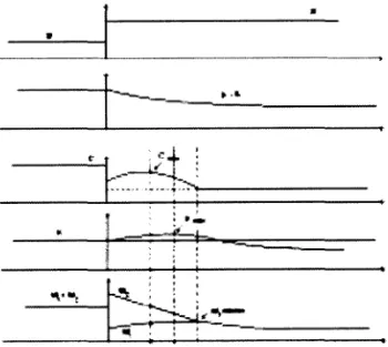
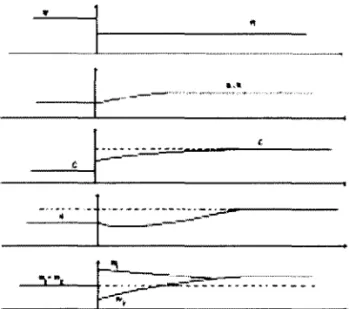
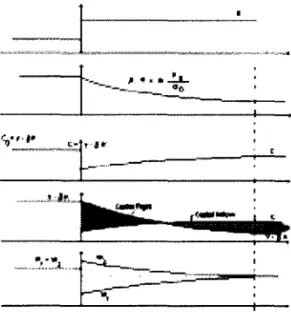
Four dynamics are studied. Firstly one studies what happens after a perma-nent rise of the rate of inflation in a closed economy. 8econdly, what occurs after a falI of inflation in a closed economy. The third and fourth dynamics are the open economy versions of the first and second dynamics. It is shown that the response of the economy to a rise of the inflation is not symmetric to its response to a falI.

The results of a permanent rise of the rate of inflation can be described starting from a long run steady state with low inflation. In the closed economy, the sudden unexpected rise of rate of inflation increases the cost of using money as working capital which induces firms to substitute administrative labor for money used as working capital. 8ince the supply of administra tive labor is fixed in the short run, there is no short run reduction in the real demand for money but there is a rise of administrative wages. 8ince the cost of administrative services increases, the demand for productive workers falls, producing a falI of productive wages. Consumption falls in response to a lower permanent income. As a result there is a positive accumulation of capital in the first phase of the transitional dynamics. During the transition to the new long run steady state, while the wage paid to administrative workers reamain above the wage of productive ones, alI the newly

•

•

•

•

•

_•

•

•

•

_•

•

•

_•

•

•

•

•

•

•

•

•

•

•

•

•

•

•

•

•

•

•

•

_•

•

•

•

_•

•

_•

•

•

•

•

•

•

•

_•

•

•

bom chose to become administrative workers. The excess supply of productive workers dampens the demand for capital, thus reducing its rate of return, which tends to increase consumption and gradually revert the positive accumulation of capital. As the supply of administrative workers is continuously increased and that of productive workers decreased, the wage deferential is gradually reduced down to zero. The average wage falIs as capital is depreciated.

As the economy approaches its new steady state with lower capital, the real return on capital tends to rise again to its previous steady state leveI. In the steady state with high infiation, the economy is poorer for the capital stock was reduced. The new leveI of wages and of consumption is lower, and a larger share of the work force is doing administrative services.

The model also casts some líght on the polítical economy of prolonged in-flationary processes. This issue is not the focus of the paper but arises as a subsidiary consequence of its results. Although in the long run all individuals lose with a higher rate of inflation, in the short run some groups profit from it. Starting at the long run non inflationary equilibrium, if (due to an exogenous reason) the group that gains with the rise of inflation gets the polítical power, inflation wiIl rise. For some time the members of this group are benefited. As time passes by however, new generations are lured to the activities that are ben-efited by infiation, thus reducing their attractiveness. As the group that benefits from infiation is enlarged in size their political clout tends to augment. More-over, as the individual gains absorbed by each of its members is whittled down by competition within the group due to its enlargement, the incentive press for rising the rate of inflation even further increases. This creates an upward in-flationary bias in which the longest the inin-flationary period the smallest is the polítical willingness to curb it. Monetary stabilization would occur only after a long period of infiation, when the economy is so impoverished that the long run gains from curbing inflation outstrips the short run loss of the group that gains with infiation.

The growth of the banking sector in inflationary economies has already been documented and modeled theoreticaIly. But high rates of inflation generate extra administrative tasks within non banking firms as weIl.

The paper is organized in 5 sections including this introduction. In the sec-ond section one presents the basic framework of the model. In the third one studies the behavior of firms and of households. In the fourth, one describes the determination of prices and the time evolution of state variables and studies the general equilibrium of the model. In the fifth section one studies the dynamic adjustment of the economy in response to changes of the rate of infiation. In the sixt section one concludes the paper.

•

•

•

•

•

•

_•

•

•

•

•

•

_•

•

•

_•

•

•

•

•

•

•

•

•

•

•

•

•

•

•

•

•

_•

•

_•

•

•

•

•

_•

•

_•

•

•

•

•

_•

•

•

2 Economic Environment

The economy is modeled in continuous time. There are three kinds of infinitely lived economic agents: the governrnent, households and firms. There is only one good that can be consumed or saved to be used as physical capital. The good is produced by firms that use as inputs physical capital, productive labor, administrative labor and money (working capital). There are two kinds oflabor: administrative and productive labor. Each household supplies labor inelasticly in one of the two labor markets. Households do not use money.

There are five competitive markets: of money, of the consumption good, of productive labor, of administrative labor, and of capital. In each of the five markets there is one price that equals supply and demando Normalizing these five prices so that the price of money is one, there remains four prices to be expressed in monetary units: the price of the consumption good

P(t) ,

the wage of productive workers

W1(t)

=

P(t)WI(t),

the wage of administrative workers

W2(t)

=

P(t)W2(t),

and the nominal rental

R(t)

=

P(t)r(t).

These four prices are fully flexible and willlater be determined in general equilibrium.

The information structure is very simple. The model has one main exogenous variable, the rate of inflation 7r, which is defined by the govemment. At any

instant

t

the prevailing rate of inflation is the best prediction for the future rates of inflation. For simplicity, instead of assuming, as is the wont in the monetary literature, that the nominal monetary supply follows an exogenous path and the rate of inflation is endogenously determined, it was assumed that the reverse holds. In the subsections below one presents the formal characterization of the economic environrnent faced by agents.

2.1 Firms

The only good of the economy is produced by competitive firms whose technol-ogy of production uses physical capital K, productive workers LI, administrative workers L2 and real money m = M/ P employed as working capital. For

simplic-ity, it is assumed that there is substitutability between capital and productive labor, but that there is a fixed proportion between productive labor and ad-ministrative services

S.

The flow of goods

Y(t)

produced at instant

t

is given by

Y(t)

= F

(K(t),

min{L1(t),

S(m(t),

L

_2(t))})

where the function F : ~2 ~ ~ describes the amount of goods produced with a given amount of physical capital and productive workers when the amount of administrative services is not binding. The technology of providing administrative services S : ~2 ~ ~ uses administrative labor and working capital represented by real money balances which will simply be called money. Both F and S are

•

•

•

•

•

•

_•

•

•

_•

•

•

_•

•

•

_•

•

•

•

•

•

•

•

_•

•

_•

•

•

•

•

•

•

•

_•

•

•

_•

•

•

•

•

•

_•

•

•

•

_•

•

•

assumed to be homogeneous of degree one, twice continuously differentiable and to satisfy the INADA conditions. Capital depreciates at the instantaneous rate 8.

2.2 Households

At each instant of time

t

a large cohort of size ÀL is bom. Each household of this cohort has a constant instantaneous probability À of dying. This implies that the probability that a household bom at instant s is alive at instant

t ,

s ~

t,

is given

by e->'(t-s). By the Law of Large Numbers, the size of the cohort s as of date

t ,

s ~

t,

is thus ÀLe->.(t-s). Hence, the size of the population at instant

t

is given by

J~oo ÀLe->.(t-s)ds

=

L. This shows that although the size of each cohort declines continuously at the rate À, the size of the population is constant.

Household receive two kinds of lump sum transfers from the govemment dur-ing its life time. The first is a once-and-for-all lump sum transfer received when the household is bom that is equal to the average wealth of those who die at that instant. The second is a continuous lump sum transfer of money that is equal to the per capita seigneurage.

Each household takes two kinds of decisions. The first decision is its career choice which is chosen at birth. This choice is irreversible thereafter. The second decision is taken continuously. It concerns its consumption and savings pattem that is determined according to the expected present value of its lifetime utility. Each household inelasticly supplies one unit of labor while alive.

Letting p

>

O stand for the instantaneous rate of time preference, the flow of consumption

c(t)

at instant

t,t

~ s, yields the flow of utility

U(c(t))

=

lnc(t).

Hence the expected present value of the household's lifetime utility is

3

Economic Choices

In this section one studies how firms and households take their economic decisions in partial equilibrium, Le., taking as given the prices of goods

P(t),

the wage of productive workers

W

1

(t)

=

P(t)Wl(t),

the wage of administrative workers

W

2(t)

=

P(t)W2(t),

and the nominal rental

R(t)

=

P(t)r(t).

The definition and study of the general equilibrium of the model is left for the next section.

3.1 Firms

Firms operate competitively. Defining the auxiliary functions

f(k)

==

F(k,

1) and s(x)

==

S(x, 1), one can determine the instantaneous flow of nominal profits that can be transferred to firms' owners. It is the difference between nominal

•

•

•

•

•

•

_•

•

•

_•

•

•

_•

•

•

_•

•

•

•

•

•

•

•

_•

•

•

•

•

•

•

•

•

•

_•

•

•

_•

•

_•

•

•

•

_•

•

_•

•

•

_•

~

revenues and nominal expenditures with capital and labor net of increases of nominal money:

where L2

(t)

is implicit1y given by

L1(t)

=

L2(t)s(m(t)j L2(t))

and M(t) denotes the increase in nominal money demando From the definition of the rate of inflation ?(t)j P(t)

=

7r, one can write M(t)j P(t)

=

m(t)

+

7rm(t). Maximization of the present value of transferable real profits at instant

t

=

T

is written as:

where the time variable

t

has been dropped from

K,

LI, L2, m,

P,

wI, W2 and r to avoid cluttering the notation.

Let KD, LP, L? and mD stand for the demands for capital, productive labor, administrative labor and real money. Optimization with respect to the capital stock yields:

(1)

where the symbol ", " represents the first derivative of the underlying func-tion.

Optimization with respect to money implies:

7r

+

r W2

s '(mD j L?) - s(mD j L?) - mD j L? s '(mD j L?)

(2)

The left hand side of (2) represents the (opportunity) cost of producing an additional unit of administrative service using more money; whilst the right hand side is that cost when more administrative labor is chosen. The necessary condi-tion for cost minimizacondi-tion is that the cost of an addicondi-tional unit of administrative service must be the same for both factors of production.

The optimum choice of productive labor gives:

( KD) KD , (KD) W2

f

Lp - Lp

f

Lp = WI

+

s(mD j L?) - mD j L? s '(mD j L?) (3)

The left hand side of (3) is the amount of goods produced by and additional productive worker, whilst the right hand side is the sum of the wage paid to the additional productive worker with the cost of an additional administrative

•

•

•

_•

•

•

•

•

•

_•

•

•

_•

•

•

_•

•

•

•

•

•

_•

•

•

•

_•

•

•

•

•

•

•

•

_•

•

•

_•

•

_•

•

•

•

_•

•

•

•

_•

•

_•

service

as

seen in (2). This equation reflects the assumption that there is a fixed proportion between productive labor and administrative services.

The demand for administrative labor is implicitly given by

(4)

3.2

Households

The first decision of a household is its career choice. Let

(3( s)

stand for the share of the cohort bom at instant s that chooses to be productive workers.

If the real wage Wl (s) of administrative workers is higher than the real wage

W2 (s)

of productive ones, alI the newly bom wiIl prefer to be productive workers, i.e., (3(s)

=

1. When

Wl(S)

<

W2(S)

alI the newly bom will prefer to be an administrative workers, i.e., (3(s)

=

O. When

Wl(S)

=

W2(S),

the new cohort will be divided between productive and administrative workers in such a way

as

to keep the two wages equal.

The mathematical expression of the share of workers that keeps both wages equal will be determined later in the section where one studies the general equi-librium. The fraction

a(t)

of the labor force that work

as

productive workers at instant

t,

is the sum of all productive workers of past cohorts that are still alive at instant t:

a(t)

=

[~

Àe->.(t-s){3(s)ds

(5)

The consumption choice at instant

t

~ S of each household of type i

=

1, 2 of

cohort S is subject to the budget constraint

8Vi(S, t)/at

=

r(t)vi(S, t)

+

Wi(S, t)

+

cp(t) - Ci(S, t),

with

Vi(S,

s) = 'IjJ(s) (6)

where

Vi(S, t)

is its wealth or accumulated net savings,

r(t)

is the real rate of return on accumulated net savings,

Wi(S, t)

is its flow of labor income,

Ci(S, t)

is its flow of consumption,

cp(

t)

is the inflationary flow of lump sum transfer received from the government, and 'IjJ( s) is the amount of reallump sum transfers received from the government at birth. The amount of these two transfers wiIl later be defined in order to coherently dose the general equilibrium of the model.

The optimal consumption choice is described by

l\(S, t)

=

Ci(S, t)[r(t) - (p

+

À)]

(7)

where the dot over a variable will denote its time derivative.

From (7) and (6), the consumption of a household of cohort S

as

of instant

t

is given by

Ci(S, t)

=

(p

+

À)

[Vi(

s,

t)

+

hi(t)

+

x(t)]

(8)

•

•

•

•

•

•

_•

•

•

_•

•

•

_•

•

•

_•

•

•

•

•

•

_•

•

•

•

•

•

•

•

•

•

•

•

_•

•

•

_•

•

•

_•

•

•

_•

•

•

•

_•

•

_•

and the condition

where

lim

e-

ft t1

r(t2)dt2Vi (S, tI)

= O

tl-+oe

(9)

hi(t)

=

hi(s, t)

=

1

0e

e-

ft

t1

r(t2)dt2Wi (S, tl)dtl

=

1

0e

e-

ft

t1

r(t2)dt2Wi(tl)dtl

(10)

is the present value of its future labor income, and

(11)

is the present value of its future inflationary transfers. Note that

hi(s,

t)

is in-variant of s since members of different cohorts that have the same occupation get the same wage.

The wealth of the cohort bom at instant s as of instant

t , v(s),

is given by

v(s)

=

(3(S)VI(S, t)

+

(1-

(3(S))V2(S, t).

The aggregate wealth

V(t)

at instant

t

is given by the sum over all cohorts alive at instant

t :

V(t)

=

L [toe v(s, t)>"e->.(t-s)ds

=

L

[~

{(3(S)VI(S, t)+(1-(3(S))V2(S, t)}>"e->.(t-s)ds

(12) Deriving (12) with respect to time, and recalling that the newly bom are equally wealthy, Le.,

VI(t, t)

=

V2(t, t)

=

'IjJ(t) ,

one gets

V(t)

=

>'L'IjJ(t) - >"V(t)

+

(13)

+L [toe {(3(s)

âVI~'

t)

+

(1 _

(3(s))

âV2~'

t) }>"e->.(t-s)ds

The first term of (13) represents the lump sum transfer to the newly bom and the second the wealth of those who die. The assumption that the wealth of those who die at instant

t

is equally divided among those who are bom at the same instant of time implies that the first two terms of (13) cancel out. Substituting (6) into (13) one gets:

V(t)

=

r(t)V(t)

+

W(t)

+

X(t) - C(t)

(14)

where

X(t)

=

x(t)L

represents the aggregate inflationary transfer to households at instant

t, W(t)

stand for the aggregate labor income at instant

t

W(t)

=

L [toe >"e->.(t-s){(3(S)WI(t)

+

(1 -

(3(s))w2(t)}ds

(15)

and

C(t)

for the aggregate consumption at instant

t

•

•

_•

•

•

•

•

•

•

_•

•

•

_•

•

•

•

_•

•

•

•

•

_•

•

_•

•

_•

•

•

_•

•

•

•

•

_•

•

•

_•

•

_•

•

•

•

_•

•

_•

•

_•

•

_•

The present value of the aggregate labor income of the households currently alive H

(t)

is given by

Deriving (17) with respect to time one gets

H(t)

=

r(t)H(t) - W(t)

+

Z(t)

(18)

where

Z(t) -

ÀL

1

00 e-ft

tl

r(t

2

_)dt

2

_{jj(t)Wl(t1)

+

_{(1 -}

_{jj(t))W2(t1)}dt1 - ÀH(t)}

₍₁₉₎

_ ÀL[jj(t) -

[too

e-À(t-S)jj(s)ds]

1

00

e-ft tl

r(t

2

)dt

2

[Wl(tl) - W2(t1)]dt1

-

ÀL[jj(t) - a(t)][h1(t) - h2(t)]

It is important to note that

Z(t)

2:

o.

When

h1(t)

>

h2(t),

all the newly bom at instant

t

chose to be productive workers, i.e.

jj(t)

= 1. Hence when

h1(t)

>

_h2(t)

one has

jj(t) - a(t)

=

1 -

a(t)

>

O. When

h1(t)

<

_h2(t),

alI the newly bom at instant

t

chose to be administrative workers, i.e.

jj(t)

= O. Hence when

h1(t)

<

h2(t),

one has

jj(t) - a(t)

= O -

a(t)

<

O.

The term Z (t) represents the part of instantaneous change of the present value of the aggregate labor income that is due to professional choices. Whenever the two wages differ, this present value is increasing because among those that die there are some that receive the high wage and others that get the low one; but all those that are bom get the high wage. This explains why

Z(t)

2:

O.

From (8), (16), (12) and (17), the aggregate consumption can be written as

C(t)

=

(À

+

p)[V(t)

+

H(t)

+

X(t)]

(20) where

X(t)

=

Lx(t).

Taking the derivative of (20) with respect to time, and substituting (14), one gets

C(t)

=

(À

+

p){[r(t)V(t)

+

W(t)

+

X(t) - C(t)]

+

H(t)

+

X(t)}

=

(À

+

p){[r(t)V(t) - C(t)]

+

{W(t)

+

H(t)}

+

{X(t)

+

X(t)]}

Substituting (18) and recalling that from (11)

X(t)

=

r(t)X(t) - X(t)

one gets

C(t)

=

(À

+

p)[r(t){V(t)

+

H(t)

+

X(t)}

+

Z(t) - C(t)]

Substituting (20) one gets

C(t)

=

[r(t) - (À

+

p)]C(t)

+

(À

+

p)Z(t)

11

•

•

_•

•

•

•

•

•

•

_•

•

•

_•

•

•

•

•

•

•

•

•

_•

•

•

•

•

•

_•

•

•

•

•

•

_•

•

•

_•

•

•

_•

•

•

_•

•

•

•

_•

•

_•

Expressions (14) and (21) summarize the aggregate savings and consumption decisions of households. These expressions will play key roles in the study of the general equilibrium ahead.

4

General Equilibrium

There are three state variables in the model: the first is the nominal supply of money

M(t),

determined by the govemmentj the second is the per capita aggre-gate supply of capital

k(t)

=

K(t)j L,

which is the counterpart of the percapita wealthj and the third is the share

a( t)

=

LI (t) j L

of households that supply labor in the productive labor market.

The general equilibrium will be studied in three steps. In the first step, one takes as given the triple of state variables

(k(t), a(t), M(t))

at instant t and studies the determination of the relative prices (r(

t),

WI

(t),

W2

(t), P( t))

that clear

the five markets. In the second step, one studies the time derivative of each of the three state variables in response to the prices that clear the markets. In the third step one defines the concept of general equilibrium and show that it is unique.

4.1 Determination of Prices for Given State Variables

Given the state variables

(k(t), a(t), M(t)),

the supply of capital

KS(t)

is the counterpart of households' assets:

KS(t)

=

V(t).

The supply of money

M(t)

is defined by the government. The supply of productive and administrative workers are respectively

Lr(t)

=

a(t)L

and L~(t) = (1 -

a(t))L.

Hence the three state variables

(M(t), k(t), a(t))

determine the supply in four markets. In the fifth market the supply of goods is given by the optimal decision of firms

yS(t)

=

Lf(t)f(KD(t)j LI(t)).

The demands for capital

KD(t),

productive workers

Lf(t),

administrative workers

Lf(t)

and money

MD(t)

are determined by the system of equations (1), (2), (3) and (4). The demand for goods is

yD(t)

=

C(t)

+

8K(t)

+

K(t).

In order to close the general equilibrium, one assumes that the lump sum transfers to households are equal to the proceeds from monetary creation X

(t)

=

M(t)j P(t)

=

m(t)

+

7rm(t).

According to Walras's law when supply equals demand in four markets, this will also hold in the fifth one. Hence the characterization of the general equilib-rium will be made imposing that supply equals demand in the capital market, in both labor markets and in the money market. Let

Jl(t)

=

m(t)j L

=

M(t)j P(t)L

(22)

stand for real per capita money. Since

M(t)

is a state variable and

L

is constant, the nominal price of the good

P(t)

is uniquely determined for a given value of

Jl( t).

Hence

Jl

can be treated as a relative price.

•

•

_•

•

•

_•

•

•

•

_•

•

_•

•

•

•

_•

•

•

•

_•

•

_•

•

•

•

'.

•

_•

•

•

•

•

•

..

•

•

•

•

_•

•

•

•

_•

•

_•

•

_•

~

•

The state variables

(k(t), a(t), M(t))

at instant

t

define the supply of capital, the supply of both kinds of labor and the supply of money. The set of four prices

(r(t), WI(t), W2(t), J.L(t))

must satisfy (1), (2), (3) and (4). Hence at each instant the following four equations must hold

f'(k/a)=r+{}

w+r

~

s

'(J.L/(1 - a))

s(J.L/(1 - a)) - J.L/(1 - a)

S

'(J.L/(1 - a))

(23)

(24)

f (k/a) - k/a f' (k/a)

=

WI

+

s(J.L/(1 _ a)) _

J.L/(~~

a)

S

'(J.L/(1 _ a))

(25)

a/(1 - a)

=

S

(J.L/(1 - a))

(26)

where the time symbol

t

has been dropped from

k(t), a(t), J.L(t) , r(t), WI(t)

and

W2 (t)

to avoid cluttering the notation.

The equilibrium in the goods market is easily checked: the zero profit condi-tion implies

where W is the labor income defined by (15). Substituting (rK

+

W

+

X) from (14), and setting V

=

K, one can write

which states that supply is equal to demand in the goods market in accordance to Walras' law.

4.2 Evolution of State Variables for Given Prices

In

this subsection one studies how the state variables

(M(t), k(t), a(t))

evolve when the rei ative prices

(r(t), WI(t), W2(t), J.L(t))

are determined byequations (23), (24), (25) and (26) .

4.2.1 Dynamics of the Share of Productive Labor

From (25) , (24) and (23), the real wage of productive workers is written as

WI =

{f

(!5.) _ !5.

f'

(!5.)} _

w

+

f '

(~)

- {}

a

a

a

S '(~) _l-a

(28)

From (26) and the concavity of the function s, one concludes that

J.L/(1- a)

is an increasing function of a. This and the concavity of the functions s and

f

assure that WI can be written as a function ofthe ratio

k/a

and

a:

WI

=

WI

(k/a, a)

with

•

•

•

•

_•

•

•

•

•

_•

•

_•

•

•

•

_•

•

•

•

•

•

_•

•

•

•

_•

•

_•

•

•

•

•

•

•

_•

•

_•

•

•

_•

•

•

_•

•

•

•

•

_•

~

partial derivatives Wl_k/_o

>

o

and Wlo

<

O. Qne concludes that Wl is increasing

in k and decreasing in a.

Likewise, the real wage of administrative workers is written as

= {

+

f '

(~)

-

8}s(6) -

6

s

'(6)

W2 7r '(-E-)

a s l-a

(29)

The concavity of the functions s and

f

assure that is W2 can be written as

a function of the ratio

k/a

and a: w2

=

W2

(k/a,

a) with partial derivatives W2_k/_o

<

O and W20

>

O. Qne concludes that Wl is decreasing in k and increasing

in a.

From

(28)

and

(29),

Wl

>

W2 if and only if:

f

(l!.)

_l!.

f'

(l!.)

1

+

s(-E-) - -E-s '(-E-)

a a a

>

l-a l-a l-a (30)

7r

+

f'

(~)

-

8 s '(6)

The right hand side of (30) is an increasing function of

J1/(l-

a). Since (26) assures that

J1/(1 -

a) is an increasing function of a, it follows that the right hand side of this equation is an increasing function of a. Hence one defines the increasing function 9 : ~ ---t ~ such that

g(

a) stands for the right hand side of

(30).

Likewise, the assumptions about the production function assure that the left hand side of (30) is an increasing function of the ratio

k/a

and a decreasing function of 7r. Hence one defines the function

q :

~2 ---t ~ such that

q(k/a,7r)

stands for the left hand side of (30), with partial derivatives qk/a

>

O and q7r

<

o.

Qne concludes that in the plan (k x a) the set of points where Wl

=

W2, for

a given

7r,

is represented by

q(k/a, 7r)

=

g(a).

It has positive slope. The INADA conditions assure that lim

g(a)

=

+00,

lim

h(k/a,7r)

= O, limg(a) =

o.

These

a--++oo k / a--+O a--+O

properties imply that the point (O, O) belongs to this locus and that this locus approaches asymptotically the vertical line a = 1.

Another property of the lo cus Wl = W2 is that it crosses the line

f '

(k / a) =

p

+

>.

+

8 at a single point. In order to see this, one starts at any point (k, a) on the line

f'

(k/a)

=

p

+

>.

+

8 and move upwards along this line. Since the ratio

k/a

remains fixed, for a given

7r,

h(k/a, 7r)

is a positive constant; while

g(a)

increases monotonically from zero at a = O to infinite as a ---t 1. Continuity of

the functions q and 9 assures the existence of a single crossing point that wiIl be denoted by (a;, k;).

Since the locus Wl = W2 moves the left as the rate of inflation increases, one

concludes that the higher the rate of inflation the smaller are a; and

k;.

In order to avoid cluttering the notation, the subscript 7r will be dropped from (a;, k;)

Another property of the locus Wl = W2 is that it remains below the line

f'

(k/a)

=

p+>'+8

for a in the range (O,

a;)

and above it in the range

(a;,

1). To see this, one starts at the crossing point

(a;, k;)

where

f

'(a;/k;)

=

p+>'+8

and

•

•

•

•

•

•

•

•

•

•

•

•

_•

•

•

•

_•

•

•

•

•

•

_•

•

•

_•

•

•

•

•

_•

•

_•

•

•

•

_•

•

•

_•

•

_•

•

•

•

•

_•

•

_•

q(a;jk;,7r)

=

g(a;)

and move downwards along the line defined by

I'

(a;jk;)

=

p

+

>.

+

8 . Take any

ex'

E (O, a;) and the corresponding k' such that the point

(k', ex')

belongs to the locus

Wl

=

W2,

i.e.,

q( k' j ex', 7r)

=

g( a').

Since 9 is increasing

g(ex')

<

g(a;)

and therefore

q(k' jex', 7r)

=

g(a')

<

g(a;)

=

q(a;jk;, 7r).

Since

q

is increasing in

kja,

one concludes that

k' ja'

<

a;jk;,

which shows that the locus

Wl

=

W2

is located below the line

I '

(kja)

=

p

+ >. +

8 for

a

in the range (O,

a;).

At any instant

t,

an amount

>.a(t)L

ofthe

_L1(t)

=

a(t)L

productive workers, die. When

Wl (t)

>

W2 (t)

all the

>'L

newly bom households decide to be pro-ductive workers. Hence the net increase in the supply of these workers is

LI

=

>'L - a(t)>'L

=

L[1 - a(t)J>..

Hence ó =

>'(1 - a(t))

>

O.

When

W2(t)

>

Wl(t)

the derivative is ó

=

->.a(t)

<

O. When

Wl(t)

=

W2(t)

the share

a

wiIl evolve in order to keep both wages equal, i.e.,

a(t)

wiIl foIlow

k(t)

in a way as to keep the state

(k(t), a(t))

on the locus

Wl

=

W2.

Points above this locus are those where

ó =

>'(1- a)

>

O, whereas points below this locus are those where ó =

->.a <

O. The locus

Wl

=

W2

is

not

a locus where

ex

=

O. The dynamics of

a

is summarized as:

If

q(k(t)ja(t), 7r)

If

q(k(t)ja(t), 7r)

If

q(k(t)ja(t), 7r)

>

g(a(t)),

then

ó(t)

=

>'(1 - a(t))

>

O

(31)

g(a(t)),

then

ó(t)

=

k qk/a{ ag'(a)

+

kja qk/a}-1

<

g(a(t)),

then

ó(t)

=

->.a(t)

<

O

One concludes that ó is positive (negative) for points (a, k) to the left (right) of the locus

Wl

=

W2.

For points on the locus

Wl

=

W2 ,

the time derivative ó is

not

zero, but has the same sign of the time derivative

k

which wiIl be studied ahead.

4.2.2 Dynamics of the Consumption Flow

Substituting (23) into (21) and dividing through by L, the dynamics of the ag-gregate per capita consumption is

ê(t)

=

[I

'(k(t)ja(t)) - (>'

+

P

+

8)Jc(t)

+

Z(t)(>.

+

p)j L

(32)

From (19), one knows that at an instant

t, Z(t)

is given by future values of the variables

_{r(t1) , Wl(tl), W2(t1)}

and

{3(td,

where

t

< tI.

These four variables are functions of the future states

(a(td, k(td).

Since

_{(a(t 1), k(t1))}

is a function of the current state

(a(t), k(t)),

one concludes that

Z(t)

is itself a function of the current state

(a(t), k(t)).

Hence one can write

Z(t)

=

Z(a(t), k(t)).

From (19), one knows that

Z(k, a) 2:

O with equality at the points where the state

(a, k)

is on the locus

Wl

=

W2.

This implies that ê =

(>'

+

p)Zj L

>

O

for points on the line

I '

(kja)

=

p

+ >. +

8. Since

(O, O)

belongs to this line and also to the locus

Wl

=

W2,

one concludes that

(O, O)

belongs to the locus ê

=

o.

•

•

_•

•

•

•

_•

•

•

_•

•

•

_•

•

•

•

•

•

•

•

•

•

_•

•

•

•

•

•

•

•

•

•

_•

•

_•

•

_•

•

•

_•

•

_•

•

•

•

•

_•

•

_•

One can now locate the locus é

=

O in the plan (k x a). Moving along the lo cus Wl = W2 , where Z(k, a) = O, one has é

>

O (é

<

O) when the state (k, a)

is on the part of the lo cus Wl

=

W2 below (above) the line

f '

(k/a)

=

p

+

À

+

8. On the line

f ' (k/a)

=

p

+

À

+

8 , one has é

=

(À

+

p)Z/ L>

o.

For

(k, a)

at the intersection of this line with the locus Wl

=

W2 , Le., at (a;, k;) one has é

=

o.

Take any point A

=

(kA, aA)

on the line

f' (k/a)

=

p

+

À

+

8 and another point B = (k B, a B) on the part of the locus Wl = W2 above (a;, k;). It has just

been shown that

é(A)

>

O and

é(B)

<

o.

From the continuity of the function

c

there is a point

D

=

(kD' aD) in the segment

AB

where

c(D)

=

o.

One concludes that the lo cus é

=

O touches the line

f '

(k / a)

=

p

+

À

+

8 at

( a;,

k;) and lies to the left of this line elsewhere. At

(a;,

k;), the locus é

=

O

crosses the locus Wl

=

W2. Points (a, k) above (below) the locus é

=

O are those

where é

<

O

(é>

O).

4.2.3 Dynamics of the Capital Stock

Setting the aggregate stock of capital

K(t)

equal to the aggregate wealth

V(t),

from (14), the dynamics of K is given by

K(t)

=

r(t)K(t)

+

W(t)

+

<I>(t) - C(t)

(33)

Substituting (27) into (33) and dividing through by L the dynamics of the per capita stock of capital is given by

k(t)

=

a(t)f(k(t)/a(t)) - 8k(t) - c(t)

(34)

One now studies the location of the locus where

k

=

O in the plan (k x a).

Along this locus the second time derivative must also be zero:

Setting

k

=

O and

k

=

O, one gets:

(36)

Equation (36) implies that the locus

k

= O is located in the region of the plan

(k x a) where the time derivatives é and ó: have the same signo This motivates the division of the plan (k x a) into four regions according to the signs of é and

a.

The first region is represented by

[a

>

O,

é

<

O].

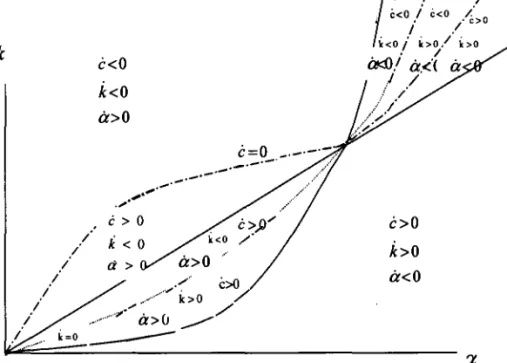
This region is bounded by the k axis, the part of the locus é

=

O situated between (O, O) and (a;, k;), and the part of the locus Wl = W2 above (a;, k;). The second region is represented

by [a

<

O, é

>

O]. This region is bounded by the a axis, the part of the locus

•

•

_•

•

•

•

•

•

_•

•

•

•

•

•

•

_•

•

•

•

•

•

•

•

•

•

_•

•

•

•

•

•

•

•

•

_•

•

_•

•

•

•

•

•

_•

•

•

•

_•

•

_•

Wl

=

W2 situated between

(O, O)

and (a;, k;), and the part of the locus

e

=

o

above (a;, k;). The third region is represented by

[ã

<

O,

e

<

O]. In this region, points (a, k) satisfy a

>

a* and k

>

k*. The left boundary of this region is the part of the locus Wl = W2 above (a*, k*) and its right boundary is the part of the

locus

e

= O above (a;, k;). The fourth region is represented by

[ã>

O,

e>

O]. In this region, points (a, k) satisfy a

<

a* and k

<

k*. The left boundary of this region is the part of the lo cus

e

=

O situated between (O, O) and (a;, k;), and its right boundary is the part of the lo cus locus Wl

=

W2 situated between

(O, O)

and

(a;, k;). Equation (36) assures that the lo cus

k

=

O is located in the third and fourth regions.

One now turns to the analysis of the first region

[ã

>

O,

e

<

O].

When the state

(a, k) is in the interior of this region or on its boundary on the locus

e

=

O, one has

k

<

O, for if one had

k

>

O, than (35) would imply that

k

>

O and the capital stock would increase indefinitely. When the state (a, k) is on the boundary on the part ofthe locus Wl

=

W2 situated between (a;, k;) and (1,

+(0),

(31) implies

that

k

and

O:

have the same signo Since

e

<

O, one has

k

<

O, for if one had

. ..

k

>

O then (35) would imply that k

>

O and the capital stock would increase indefinitely. Hence, on the first region

[ã >

O,

e

<

O] one has

k

<

o.

One now turns to the analysis of the second region

[ã <

O,

e>

O]. When the state (a, k) is in the interior of this region or on its boundary on the locus

e

=

O, one has

k

>

O, for if one had

k <

O, than (35) would imply that

k

<

O and the capital stock would decrease down to zero. When the state (a, k) is on the boundary on the part of the locus Wl

=

W2 situated between

(O, O)

and (a;, k;),

then (31) implies that

k

and

O:

have the same signo Since

e

>

O, one has

k

>

O, for if one had

k

<

O than (35) would imply that

k

<

O and the capital would decrease down to zero. Hence on the second region

[ã

<

O,

e>

O] one has

k

>

O.

The lo cus

k

=

O which has been shown to be in the third and fourth regions can now be located using the fact that the derivative

k

is a continuous function of the state (a,k). One starts with the third region

[O: < O,e < O].

On the left boundary of this region where Wl

=

W2 one has

k

<

O; while on the right

boundary where

e

= O one has

k

>

O. Continuity of

k

implies that

k

= O is somewhere in the interior of this region.

Likewise, on the left boundary of the fourth region

[ã

>

O,

e>

O] where

e

=

O one has

k

<

O; while on the right boundary where Wl = W2 one has

k

>

O.

Continuity of

k

implies that

k

=

O is located somewhere in the interior of this region. Points above (below) the locus

k

=

O are those where

k

<

O

(k

>

O).

But the location of the locus

k

=

O in the fourth region can be stablished more precisely. One will show that

k

=

O in this region is located to the right of the line

f '

(k

j

a)

=

p

+

>.

+

8. This is done in two steps. In the fir~t step, one shows that in the vicinity of (a;, k;) in the fourth region the locus k

=

O is located below the line

f

'(kja)

=

p

+

>.

+

8. In the second s~ep, one shows that, starting below this line in the vicinity of (a;, k;) , the locus k

=

O does not cross