TCD
7, 4681–4701, 2013Sea ice detection with space-based
LIDAR
S. Rodier et al.
Title Page
Abstract Introduction
Conclusions References
Tables Figures
◭ ◮
◭ ◮
Back Close
Full Screen / Esc
Printer-friendly Version Interactive Discussion
Discussion
P
a
per
|
D
iscussion
P
a
per
|
Discussion
P
a
per
|
Discuss
ion
P
a
per
|
The Cryosphere Discuss., 7, 4681–4701, 2013 www.the-cryosphere-discuss.net/7/4681/2013/ doi:10.5194/tcd-7-4681-2013
© Author(s) 2013. CC Attribution 3.0 License.
Geoscientiic Geoscientiic
Geoscientiic Geoscientiic
Open Access
The Cryosphere Discussions
This discussion paper is/has been under review for the journal The Cryosphere (TC). Please refer to the corresponding final paper in TC if available.
Sea ice detection with space-based LIDAR
S. Rodier1, Y. Hu2, and M. Vaughan2
1
SSAI, NASA Langley Research Center, MS 475, Hampton VA 23681-2199, USA
2
NASA Langley Research Center, MS 475, Hampton VA 23681-2199, USA
Received: 30 May 2013 – Accepted: 16 July 2013 – Published: 13 September 2013
Correspondence to: S. Rodier ([email protected])
TCD
7, 4681–4701, 2013Sea ice detection with space-based
LIDAR
S. Rodier et al.
Title Page
Abstract Introduction
Conclusions References
Tables Figures
◭ ◮
◭ ◮
Back Close
Full Screen / Esc
Printer-friendly Version Interactive Discussion
Discussion
P
a
per
|
D
iscussion
P
a
per
|
Discussion
P
a
per
|
Discuss
ion
P
a
per
|
Abstract
Monitoring long-term climate change in the Polar Regions relies on accurate, detailed and repeatable measurements of geophysical processes and states. These regions are among the Earth’s most vulnerable ecosystems, and measurements there have shown rapid changes in the seasonality and the extent of snow and sea ice coverage. 5
The authors have recently developed a promising new technique that uses lidar surface measurements from the Cloud-Aerosol Lidar and Infrared Pathfinder Satellite Obser-vations (CALIPSO) mission to infer ocean surface ice-water phase. CALIPSO’s 532 nm depolarization ratio measurements of the ocean surface are uniquely capable of pro-viding information about the ever-changing sea surface state within the Polar Regions. 10
With the finer resolution of the CALIPSO footprint (90 m diameter, spaced 335 m apart) and its ability to acquire measurements during both daytime and nighttime orbit seg-ments and in the presence of clouds, the CALIPSO sea ice product provides fine-scale information on mixed phase scenes and can be used to assess/validate the estimates of sea-ice concentration currently provided by passive sensors. This paper describes 15
the fundamentals of the CALIPSO sea-ice detection and classification technique. We present retrieval results from a six-year study, which are compared to existing data sets obtained by satellite-based passive remote sensors.
1 Introduction
Much work in recent years has been dedicated to tracking the Earth’s decreasing ice 20
cover. As reported in the 2012 Arctic Report Card (Perovich et al., 2012), the Arctic experienced the largest recorded loss of sea ice extent from March to September of 2012. Historically, the month of March is when the maximum sea-ice extent is reached and September being the minimum. By the end of the recent summer melt season satellite records (active since 1979) indicated that September 2012 ice extent was the 25
TCD
7, 4681–4701, 2013Sea ice detection with space-based
LIDAR
S. Rodier et al.
Title Page
Abstract Introduction
Conclusions References
Tables Figures
◭ ◮
◭ ◮
Back Close
Full Screen / Esc
Printer-friendly Version Interactive Discussion
Discussion
P
a
per
|
D
iscussion
P
a
per
|
Discussion
P
a
per
|
Discuss
ion
P
a
per
|
2012). With increased ice melt, a transition towards a thinner, younger ice cover is occurring (e.g., Kwok, 2007; Maslanik et al., 2007), and the formation of melt ponds on first-year sea ice reduces its albedo and increases the solar energy input and melt rate of the underlying ice (Polashenski, et al., 2008). At the end of summer 2011, only 25 % of the Arctic sea ice was more than two years old, compared to 50–60 % 5
during the 1980s (Stroeve et al., 2012). Almost none of the oldest and thickest ice (at least five years old) remains (3 % in February 2012 compared to 30–40 % in the 1980s) (e.g., Francis and Vavrus, 2012). This shift from a multiyear to seasonal ice cover has significant implications for the heat and mass budget of the ice and for the Artic ecosystems.
10
Since launching in April 2006, the principal objective of the Cloud-Aerosol Lidar and Infrared Pathfinder Satellite Observations (CALIPSO) mission has been study-ing the climate impact of clouds and aerosols in the atmosphere (Winker et al., 2010). The primary instrument aboard CALIPSO is CALIOP (i.e., the Cloud Aerosol Lidar with Orthogonal Polarization), a two-wavelength (532 nm and 1064 nm) polarization-15
sensitive (at 532 nm) elastic backscatter lidar (Hunt et al., 2009). Recent work by Rodier et al. (2012) has demonstrated that, in addition to the cloud and aerosol pa-rameters that make up CALIOP’s standard suite of data products (Winker et al., 2009), the CALIOP daytime and nighttime measurements can also be used to infer ocean surface ice-water phase. Numerous studies have shown that lidar backscattering de-20
polarization measurements can be used to distinguish between liquid and solid phases of water in the atmosphere (Sassen, 1991; Intrieri et al., 2002; Hu et al., 2009). In this
study the depolarization ratio, δ, is defined as δ=β⊥/βk, where β⊥ and βk are the
are the backscatter intensities measured with respect to the polarization plane of the
linearly polarized laser transmitter (Alvarez et al., 2006). The parallel (k) component of
25
the backscatter retains its original polarization state, while the so-called perpendicular
(⊥) component does not (Gimmestad, 2008). Here, analyses of collocated CALIPSO
TCD
7, 4681–4701, 2013Sea ice detection with space-based
LIDAR
S. Rodier et al.
Title Page
Abstract Introduction
Conclusions References
Tables Figures
◭ ◮
◭ ◮
Back Close
Full Screen / Esc
Printer-friendly Version Interactive Discussion
Discussion
P
a
per
|
D
iscussion
P
a
per
|
Discussion
P
a
per
|
Discuss
ion
P
a
per
|
provide strong evidence for this relationship between surface echo depolarization and surface ice–water state. Seasonal variability of sea ice concentration and ice extent has been monitored by many of the A-Train satellites such as the AMSR-E, and the Moderate-resolution Imagining Spectroradiometer (MODIS). The finer resolution of the CALIPSO footprints (90 m diameter, spaced 335 m apart) and its ability to retrieve sur-5
face ice-water phase beneath moderate cloud cover (optical depths<3) can provide
detailed insights into sea ice formation and dissipation that will allow more accurate interpretation of the existing data sets, especially during the during the season tran-sition months. Because CALIPSO’s measurements are not limited to daytime or clear sky conditions, the CALIPSO sea ice product can provide “fill-in” measurements where 10
other data products are limited due to instrument characteristics or have the practice of masking land surfaces. Prediction models may also benefit from the finer resolution in discriminating ice boundaries.
2 Retrieval methodology
When the CALIPSO orbit transects surfaces covered by ice, be it land or ocean, the 15
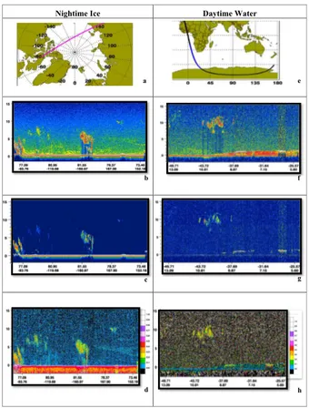
backscattered signal intensity from the surface is very strong and will frequently cause digitizer saturation. This response will be very evident in the two 532 nm channels (parallel and perpendicular) at and immediately below the Earth’s surface. When the signals from these channels are ratioed, the resulting depolarization values are in the range of 0.55–1.1. Conversely, when CALIPSO transects surfaces covered by water, 20
the signal intensity is substantially reduced, most especially in the perpendicular chan-nel, and the resulting depolarization values typically lie between 0.0–0.2. As illustrated
in Fig. 1, it is this specific effect that enables the 532 nm depolarization data to be
used for ice classification purposes. The left column of Fig. 1b, c, and d illustrates the measured backscatter from an ice surface. Each image shows a small section of the 25
nighttime orbit over the Arctic starting at 77◦N and descending to 73◦N on 14
TCD
7, 4681–4701, 2013Sea ice detection with space-based
LIDAR
S. Rodier et al.
Title Page
Abstract Introduction
Conclusions References
Tables Figures
◭ ◮
◭ ◮
Back Close
Full Screen / Esc
Printer-friendly Version Interactive Discussion
Discussion
P
a
per
|
D
iscussion
P
a
per
|
Discussion
P
a
per
|
Discuss
ion
P
a
per
|
backscatter from 2 km below the surface to 15 km above the surface. In each of the im-ages the estimated surface elevation, derived from a digital elevation map, is displayed as a red line. Surrounding this red line, the saturated values appear as multi-layered “ribbon”. The attenuated backscatter samples from this “ribbon” section will be used in the global assessment of ocean surface ice-water phase study. The right column of 5
Fig. 1d, e, and f illustrates a water transect with a section of ascending daytime orbit
starting at−49◦S to −24◦S from 14 December 2010 between 13:30 and 13:35 UTC.
The differences in measured surface depolarization due to surface type are clearly
seen in images d and h: the polar icecaps measured in image d show surface
depo-larization ratios well in excess of 0.6 (actual values are 0.747±0.0425), whereas the
10
depolarization ratios in the subtropical open ocean shown in image h are uniformly
below 0.1 (actual values are 0.024±0.028). Also illustrated in Fig. 1b, c and d is an
example of the non-ideal transient recovery of the 532 nm detectors due to very strong signal returns. In extreme cases, the non-ideal transient recovery can make it wrongly appear as if the laser signal is penetrating the surface to a depth of several hundreds 15
of meters (McGill et al., 2007). Because identical detectors with essentially identical transient recovery behaviors are used on both 532 nm channels, highly reflective ice surfaces readily induce non-ideal transient responses in both 532 nm signal returns (Hunt et al., 2009). On the other hand, the darker, less reflective water surfaces (e.g., see Fig. 1f, g and h) generate substantially weaker backscatter returns, and thus the 20
effects of this non-ideal recovery are reduced to a negligible level.
The 532 nm depolarized surface return is not reported in the existing CALIPSO data products, but instead is derived from the detected CALIOP surface echo every 335 m along track. The CALIOP surface detection algorithm (Vaughan et al., 2009) uses the Global 30 Arc-Second Elevation Data Set (GTOPO30; see http://eros.usgs.gov/#/ 25
TCD
7, 4681–4701, 2013Sea ice detection with space-based
LIDAR
S. Rodier et al.
Title Page
Abstract Introduction
Conclusions References
Tables Figures
◭ ◮
◭ ◮
Back Close
Full Screen / Esc
Printer-friendly Version Interactive Discussion
Discussion
P
a
per
|
D
iscussion
P
a
per
|
Discussion
P
a
per
|
Discuss
ion
P
a
per
|
the top and base altitudes have been retrieved from the Level 2 335 m Cloud Layer product, which is the highest resolution product produced by the CALIPSO team. We then inspect the corresponding Level 1 attenuated backscatter profile product, and
re-trieve the range-resolved 532 nm parallel (βk(z)) and perpendicular (β⊥(z)) attenuated
backscatter measurements from two consecutive altitude bins above the top altitude 5
of the surface spike to five altitude bins below the base of the surface spike, thereby compensating for possible detection errors in the CALIPSO standard algorithm and/or GTOPO30. These data are screened for fill values, integrated and ratioed, creating a surface integrated depolarization ratio, defined as follows:
δsurface= base
X
k=top
β⊥(zk)
,base
X
k=top
βk(zk) (1)
10
When harvesting the Level 1 data, additional surface properties such as DEM altitude, International Geosphere/Biosphere Programme (IGBP) surface classification and Na-tional Snow and Ice Data Center (NSIDC) snow and ice coverage (re-averaged to
CERES footprint ∼30 km) are retrieved as references. To quantify signal attenuation
by clouds and/or aerosols above the surface measurements, estimates of the 1064 nm 15
column optical depths are calculated and stored on a shot-by-shot basis.
3 Assessment of the CALIPSO lidar surface return classification technique
Initial verification that the CALIPSO depolarization surface returns can be used to dis-criminate surface ice-water phase requires that each measured depolarization ratio be compared to a product that specializes in ice classification. We therefore have collo-20
TCD
7, 4681–4701, 2013Sea ice detection with space-based
LIDAR
S. Rodier et al.
Title Page
Abstract Introduction
Conclusions References
Tables Figures
◭ ◮
◭ ◮
Back Close
Full Screen / Esc
Printer-friendly Version Interactive Discussion
Discussion
P
a
per
|
D
iscussion
P
a
per
|
Discussion
P
a
per
|
Discuss
ion
P
a
per
|
pixel. Once a match was found, a location offset from the CALIOP footprint was
calcu-lated and stored. Only samples with a longitude offset less than 0.11◦ (approximately
12 km) were included in the retrieval. The AE_SI12 product includes daily averages for sea ice concentrations and snow depth over sea ice at a 12.5 km spatial resolution (Comiso et al., 2003). From the AMSR-E data, the ice concentration, ice concentration 5
uncertainties, and snow depth are retrieved for comparative analysis and validation. The comparison data set was restricted to include only those calculated depolarization ratios between 0.0 and 1.2 for which the location of the CALIPSO footprint was within the bounds of the 12 km AMSR-E pixel. This consisted of 29,7 679 034 samples for the Northern Latitudes, for which 99 % of the depolarization ratios were between 0.0 and 10
1.2. Depolarization values normally do not exceed 1.0 unless the detectors receive a very strong signal return.
As an initial test of our concept we constructed a histogram using all 532 nm de-polarization measurements that were collocated with AMSR-E classifications during 2010. All collocated samples classified by AMSR-E as water, open water, or ice with 15
an ice concentration greater than 30 % were retrieved and tested. Figure 2 illustrates a distinctive bimodal histogram with distributions from 0.0 to 0.2 and 0.55 to 1.1. Upon examination, we found that pixels classified as water by AMSR-E correlated to depo-larization ratios in the range of 0.0 to 0.2 at a rate of 95.2 %, and pixels classified as ice correlated to depolarization ratios in the range of 0.55 to 1.1 at a rate of 98.0 %. 20
3.1 Northern Hemisphere analysis
Using this newly-defined ice and water classification criteria, samples from July 2006 through September 2011 (i.e., the time period when CALIPSO and AMSR-E had coin-cidental measurements) were retrieved and grouped for additional testing. Each depo-larization value was compared to its collocated AMSR-E pixel classification, generating 25
TCD
7, 4681–4701, 2013Sea ice detection with space-based
LIDAR
S. Rodier et al.
Title Page
Abstract Introduction
Conclusions References
Tables Figures
◭ ◮
◭ ◮
Back Close
Full Screen / Esc
Printer-friendly Version Interactive Discussion
Discussion
P
a
per
|
D
iscussion
P
a
per
|
Discussion
P
a
per
|
Discuss
ion
P
a
per
|
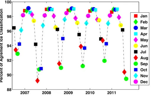
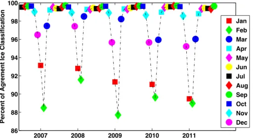
in the winter months and a lower percentage of agreement in the transitional summer-fall months. For 61 of the 63 months of our data sample, when AMSR-E classified the pixel as ice, the calculated depolarization values fell in the range of 0.55 to 1.1 at a rate of 90 % or higher. The two months that did not measure above 90 % agreement were August 2007, when the rate was 89.2 %, and September 2011, when the rate was 5
89.5 %.
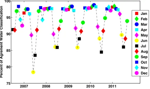
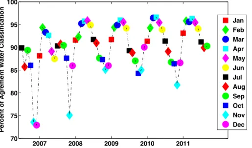
Next we looked at the consistency of the water classification for samples in the north-ern latitudes. As seen in Fig. 4, a seasonal trend is also evident, with a higher percent-age of agreement in the winter months and a lower percentpercent-age of agreement in the summer months. For 51 of the 63 months, when AMSR-E classified the pixel as water, 10
the calculated depolarization values fell in the range of 0.0 to 0.2 at a rate of 90 % or higher. For 60 of the 63 months the agreement was 85 % or higher. The summer months, specifically June and July 2007 through 2011 showed the lowest agreement.
Though the summer and transitional months recorded the lowest percentage of scene classification agreement for both of the two classification test cases, it does 15
highlight the possibility of CALIPSO’s depolarization values providing fractional scene classification. A maximum of 36 CALIPSO 335 m surface depolarization samples could fall within each 12 km AMRS-E pixel and provide additional information about sea sur-face classification. When examining the collocated records that indicated a mismatch for ice classification, it was found that 85 % of those records contain AMSR-E pixels 20
with ice concentrations in the range of 10 % to 80 % indicating a mix-phase scene of ice and water. When examining the non-matching collocated records for water classi-fication it was found that 80 % of those records also contained ice concentrations in the range of 10 % to 80 %. The non-matching due to a mixed-phase scene was not unexpected. In this study our scene matching criteria required 100 % agreement be-25
TCD
7, 4681–4701, 2013Sea ice detection with space-based
LIDAR
S. Rodier et al.
Title Page
Abstract Introduction
Conclusions References
Tables Figures
◭ ◮
◭ ◮
Back Close
Full Screen / Esc
Printer-friendly Version Interactive Discussion
Discussion
P
a
per
|
D
iscussion
P
a
per
|
Discussion
P
a
per
|
Discuss
ion
P
a
per
|
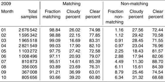
Additional analysis was performed to determine if cloud cover contributed to the mismatch in scene classification. Data from the October 2009 ice classification data set was selected for the initial test. Of the 805 656 valid collocated samples in this subset, 94 % showed agreement between the CALIPSO and AMSR-E scene classifications. 40 % of these matching scenes contain one or more cloud layers, whereas 60 % of 5
the matching scenes were classified as clear sky. The remaining 6 % of October 2009 ice classification valid samples had been classified as non-matching with 68 % having clear sky and 31 % having one or more cloud layers. Table 1 lists the percentages of cloudy and clear sky samples for each month of 2009.
The similar distributions of cloudy and clear sky samples for the matching and non-10
matching ice classification scenes seen in Table 1 strongly suggest that clouds do not contribute to the mismatch in scene classification.
From our analysis, the prevailing reason for a mismatch in the scene classification is not due to cloud cover, but instead from attempting to match a 335 m CALIPSO sample to a 12 km AMSR-E pixel that is observing a mixed-phase scene. CALIOP’s ability to 15
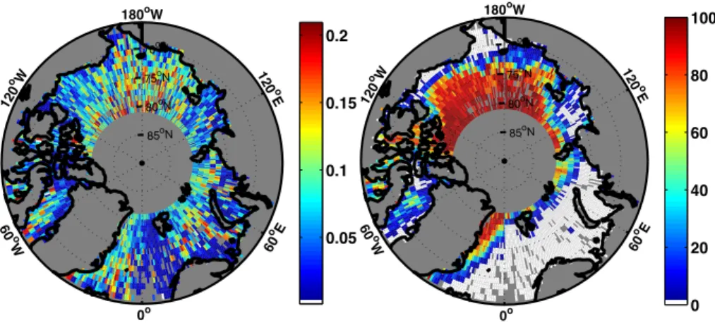
pinpoint the locations of pockets of water (newly formed melt ponds) in AMSR-E pixels classifies as ice (or, conversely, to locate chunks of ice in pixels that AMSR-E classifies as water) is illustrated in the July 2011 Artic circle plots (Fig. 5a and b).
Figure 5a represents the CALIOP footprints for July 2011 with depolarization values less than 0.2, and thus classified as water. Figure 5b is the AMSRE classification for 20
the collocated pixel. The AMSRE plot ranges from 100 % ice, seen in dark red, to zero percent ice, or water, which is represented as white. Of interest is the area between
120◦W to 120◦E where AMSRE indicates 90–100 % ice and CALIOP has detected
water. CALOIP’s detection ability would be an asset to the community for uncertainty analysis and detailed scene classification.
25
3.2 Southern Hemisphere analysis
TCD
7, 4681–4701, 2013Sea ice detection with space-based
LIDAR
S. Rodier et al.
Title Page
Abstract Introduction
Conclusions References
Tables Figures
◭ ◮
◭ ◮
Back Close
Full Screen / Esc
Printer-friendly Version Interactive Discussion
Discussion
P
a
per
|
D
iscussion
P
a
per
|
Discussion
P
a
per
|
Discuss
ion
P
a
per
|
agreement in the winter months and a slightly lower percentage of agreement for the summer months of January and February. For 58 of the 63 months of our data sample, when AMSR-E classified the pixel as ice, the calculated depolarization values fell in the range of 0.55 to 1.1 at a rate of 90 % or higher. However February 2007, 2009, 2010, 2011 and January 2011, all austral summer months, had an agreement between 88 % 5
and 89 %.
A seasonal trend is also evident when analyzing the agreement for water classifica-tions Fig. 7. a higher percentage of agreement is seen in the winter months and again a lower percentage of agreement for the summer months. For 37 of the 63 months, when AMSR-E classified the pixel as water, the calculated depolarization values fell in 10
the range of 0.0 to 0.2 at a rate of 90 % or higher. For 58 of the 63 months the agree-ment was 85 % or higher. The season transition months, specifically November 2006 through 2011 showed the lowest agreement.
3.3 Water verification
Additional verification of the depolarization range for water classification was performed 15
by selecting all data samples for July 2010 between latitude bands 20 north–20 south and grouping them by the International Geosphere/Biosphere Programme (IGBP) (wa-ter) and the SDP Toolkit/HDF-EOS Land-Water Mask subtypes for analysis. 3 783 330 samples were classified by IGBP as water and 99.83 % of these had depolarization ratios between 0.0 and 0.21 with a mean value of 0.012 and a standard deviation of 20
TCD
7, 4681–4701, 2013Sea ice detection with space-based
LIDAR
S. Rodier et al.
Title Page
Abstract Introduction
Conclusions References
Tables Figures
◭ ◮
◭ ◮
Back Close
Full Screen / Esc
Printer-friendly Version Interactive Discussion
Discussion
P
a
per
|
D
iscussion
P
a
per
|
Discussion
P
a
per
|
Discuss
ion
P
a
per
|
4 Summary
In this paper we describe a new application of the CALIPSO 532 nm attenuated backscatter data to provide additional observations in the Polar Regions. We have shown that the retrieval of the 532 nm surface depolarization provides an accurate classification of the sea surface scenes. This retrieval can be performed with samples 5
acquired during the CALIPSO day and nighttime orbits, and with samples that contain one or more cloud layers.
The AMSR-E 12 km L3 ice concentration data products provided the standard for our comparison of the newly defined CALIPSO surface ice-water classification technique. After analyzing 63 months of collocated samples we found that our method accurately 10
classified the surface scene at a rate of 90 % or higher. We note that our success rate had a seasonal variance, with a higher percentage of matching during the height of winter and lowest during the summer and transitional months. This trend was espe-cially noticeable during the summer of 2007 when the arctic experienced one of the largest melts in recent history. We believe that our scene classification methodology 15
produced from the 335 m footprint could be an asset during these transitional months. The ability to detect the changing ice-water composition at a finer detail would provide an enhanced detailed scene composition. Additionally, with CALIPSO’s measurements not being limited to daytime or clear sky conditions it could provide a “fill-in” measure-ment where other data products are limited due to instrumeasure-ment characteristics or have 20
the practice of masking land surfaces. Prediction Models may also benefit from the finer resolution in discriminating ice boundaries.
References
Alvarez, J. M., Vaughan, M. A., Hostetler, C. A., Hunt, W. H., and Winker, D. M.: Calibra-tion Technique for PolarizaCalibra-tion-Sensitive Lidars, J. Atmos. Oceanic Technol., 23, 683–699, 25
TCD
7, 4681–4701, 2013Sea ice detection with space-based
LIDAR
S. Rodier et al.
Title Page
Abstract Introduction
Conclusions References
Tables Figures
◭ ◮
◭ ◮
Back Close
Full Screen / Esc
Printer-friendly Version Interactive Discussion
Discussion
P
a
per
|
D
iscussion
P
a
per
|
Discussion
P
a
per
|
Discuss
ion
P
a
per
|
Comiso, J. C.: Warming trends in the Arctic from clear sky satellite observations, J. Climate, 16, 3498–3510, doi:10.1175/15200442(2003)016<3498:WTITAF>2.0.CO;2, 2003.
Francis, J. A. and Vavrus, S. J.: Evidence linking Arctic amplification to extreme weather in mid-latitudes, Geophys. Res. Lett., 39, L06801, doi:10.1029/2012GL051000, 2012.
Gimmestad, G. G.: Reexamination of depolarization in lidar measurements, Appl. Opt., 47, 5
3795–3802, doi:10.1364/AO.47.003795, 2008.
Hu, Y., Winker, D., Vaughan, M., Lin, B., Omar, A., Trepte, C., Flittner, D., Yang, P., Sun, W., Liu, Z., Wang, Z., Young, S., Stamnes, K., Huang, J., Kuehn, R., Baum, B., and Holz, R.: CALIPSO/CALIOP cloud phase discrimination algorithm, J. Atmos. Ocean. Techn., 26, 2293–2309, doi:10.1175/2009JTECHA1280.1, 2009.
10
Hunt, W. H., Winker, D. M., Vaughan, M. A., Powell, K. A., Lucker, P. L., and Weimer, C.: CALIPSO lidar description and performance assessment, J. Atmos. Ocean. Tech., 26, 1214– 1228, doi:10.1175/2009JTECHA1223.1, 2009.
Intrieri, J. M., Shupe, M. D., Uttal, T., and McCarty, B. J.: An annual cycle of Arctic cloud characteristics observed by radar and lidar at SHEBA, J. Geophys. Res., 107, C7, 15
doi:10.1029/2000JC000423, 2002.
Kwok, R.: Near zero replenishment of the Arctic multiyear sea ice cover at the end of 2005 summer, Geophys. Res. Lett., 34, L05501, doi:10.1029/2006GL028737, 2007.
Nagle, F. W. and Holz, R. E.: Computationally efficient methods of collocating satel-lite, aircraft, and ground observations, J. Atmos. Ocean. Tech., 26, 1585–1595, 20
doi:10.1175/2008JTECHA1189.1, 2009.
Maslanik, J. A., Fowler, C., Stroeve, J., Drobot, S., Zwally, J., Yi, D., and Emery, W.: a younger, thinner Arctic ice cover: increased potential for rapid, extensive sea-ice loss, Geophys. Res. Lett., 34, L24501, doi:10.1029/2007GL032043, 2007.
McGill, M. J., Vaughan, M. A., Trepte, C. R., Hart, W. D., Hlavka, D. L., Winker, D. M., and 25
Kuehn, R.: Airborne validation of spatial properties measured by the CALIPSO lidar, J. Geo-phys. Res., 112, D20201, doi:10.1029/2007JD008768, 2007.
Nagle, F. W. and Holz, R. E.: Computationally efficient methods of collocating satel-lite, aircraft, and ground observations, J. Atmos. Ocean. Tech., 26, 1585–1595, doi:10.1175/2008JTECHA1189.1, 2009.
30
TCD
7, 4681–4701, 2013Sea ice detection with space-based
LIDAR
S. Rodier et al.
Title Page
Abstract Introduction
Conclusions References
Tables Figures
◭ ◮
◭ ◮
Back Close
Full Screen / Esc
Printer-friendly Version Interactive Discussion
Discussion
P
a
per
|
D
iscussion
P
a
per
|
Discussion
P
a
per
|
Discuss
ion
P
a
per
|
Perovich, D. K. and Polashenski, C.: Albedo evolution of seasonal Arctic sea ice, Geophys. Res. Lett., 39, L08501, doi:10.1029/2012GL051432, 2012b.
Perovich, D., Meier, W., Tschudi, M., Gerland, S., and Richter-Meng, J.: Sea Ice (in Arctic Report Card 2012), available at: http://www.arctic.noaa.gov/reportcard, 2012.
Polashenski, C., Perovich, D., and Courville, Z.: The mechanisms of sea ice melt pond formation 5
and evolution, J. Geophys. Res., 117, C01001, doi:10.1029/2011JC007231, 2012.
Rodier, S. D., Hu, Y.-X., and Vaughan, M. A.: CALIPSO surface return for ice and water de-tection, in: Reviewed and Revised Papers Presented at the 25th International Laser Radar Conference, edited by: Papayannis, A., Balis, D., and Amiridis, V., 801–804, 2012.
Sassen, K.: The polarization lidar technique for cloud research: a review and 10
current assessment, B. Am. Meteorol. Soc., 72, 1848–1866, doi:10.1175/1520-0477(1991)072<1848:TPLTFC>2.0.CO;2, 1991.
Stroeve, J. C., Serreze, M. C., Holland, M. M., Kay, J. E., Malanik, J., and Barrett, A. P.: The Arctic’s rapidly shrinking sea ice cover: a research synthesis, Climatic Change, 110, 1005– 1027, doi:10.1007/s10584-011-0101-1, 2012.
15
Vaughan, M., Powell, K., Kuehn, R., Young, S., Winker, D., Hostetler, C., Hunt, W., Liu, Z., McGill, M., and Getzewich, B.: Fully automated detection of cloud and aerosol lay-ers in the CALIPSO lidar measurements, J. Atmos. Ocean. Tech., 26, 2034–2050, doi:10.1175/2009JTECHA1228.1, 2009.
Winker, D. M., M. A. Vaughan, A. H. Omar, Y. Hu, K. A. Powell, Z. Liu, W. H. Hunt, and S. 20
A. Young: “Overview of the CALIPSO Mission and CALIOP Data Processing Algorithms”, J. Atmos. Oceanic Technol., 26, 2310–2323, doi:10.1175/2009JTECHA1281.1, 2009.
Winker, D. M., Pelon, J., Coakley Jr., J. A., Ackerman, S. A., Charlson, R. J., Colarco, P. R., Fla-mant, P., Fu, Q., Hoff, R., Kittaka, C., Kubar, T. L., LeTreut, H., McCormick, M. P., Megie, G., Poole, L., Powell, K., Trepte, C., Vaughan, M. A., and Wielicki, B. A.: The CALIPSO mis-25
TCD
7, 4681–4701, 2013Sea ice detection with space-based
LIDAR
S. Rodier et al.
Title Page
Abstract Introduction
Conclusions References
Tables Figures
◭ ◮
◭ ◮
Back Close
Full Screen / Esc
Printer-friendly Version Interactive Discussion
Discussion
P
a
per
|
D
iscussion
P
a
per
|
Discussion
P
a
per
|
Discuss
ion
P
a
per
|
Table 1.The percentage of cloudy and clear sky samples for matching ice classification scenes
and nonmatching ice classification scenes for each month of 2009.
2009 Matching Non-matching
Month Total Fraction Cloudy Clear Fraction Cloudy Clear
samples matching percent percent non- percent percent matching
01 2 676 542 98.84 26.02 74.98 1.16 27.56 72.44
02 1 595 342 98.88 22.15 77.85 1.12 29.42 70.58
03 1 965 518 99.09 16.69 83.31 0.91 28.45 71.55
04 2 821 549 99.03 17.90 82.10 0.97 23.04 76.96
05 1 103 272 97.75 27.42 72.58 2.25 18.43 81.57
06 1 008 496 97.11 20.93 79.07 2.88 17.94 82.06
07 810 873 95.51 14.61 85.39 4.49 11.30 88.70
08 356 005 93.89 23.69 76.31 6.11 15.61 84.39
09 367 008 91.21 36.99 63.01 8.79 25.46 74.54
TCD
7, 4681–4701, 2013Sea ice detection with space-based
LIDAR
S. Rodier et al.
Title Page
Abstract Introduction
Conclusions References
Tables Figures
◭ ◮
◭ ◮
Back Close
Full Screen / Esc
Printer-friendly Version Interactive Discussion
Discussion
P
a
per
|
D
iscussion
P
a
per
|
Discussion
P
a
per
|
Discuss
ion
P
a
per
|
Nightime Ice Daytime Water
b f
a e
c g
d h
Fig. 1. (b and f) CALIOP 532 nm Total attenuated backscatter, (c and g) CALIOP 532 nm
TCD
7, 4681–4701, 2013Sea ice detection with space-based
LIDAR
S. Rodier et al.
Title Page
Abstract Introduction
Conclusions References
Tables Figures
◭ ◮
◭ ◮
Back Close
Full Screen / Esc
Printer-friendly Version Interactive Discussion
Discussion
P
a
per
|
D
iscussion
P
a
per
|
Discussion
P
a
per
|
Discuss
ion
P
a
per
|
−00.2 0 0.2 0.4 0.6 0.8 1 1.2
0.5 1 1.5 2 2.5 3 3.5x 10
6
WATER MIX ICE
Fig. 2.The CALIOP 532 nm Depolarization ratio distributions for 2010 when a surface echo
TCD
7, 4681–4701, 2013Sea ice detection with space-based
LIDAR
S. Rodier et al.
Title Page
Abstract Introduction
Conclusions References
Tables Figures
◭ ◮
◭ ◮
Back Close
Full Screen / Esc
Printer-friendly Version Interactive Discussion
Discussion
P
a
per
|
D
iscussion
P
a
per
|
Discussion
P
a
per
|
Discuss
ion
P
a
per
|
2007 2008 2009 2010 2011
88 90 92 94 96 98 100
Percent of Agrement Ice Classification
Jan Feb Mar Apr May Jun Jul Aug Sep Oct Nov Dec
Fig. 3.Northern Latitudes for 2006 to 2011 monthly percentage of agreement when AMSR-E
TCD
7, 4681–4701, 2013Sea ice detection with space-based
LIDAR
S. Rodier et al.
Title Page
Abstract Introduction
Conclusions References
Tables Figures
◭ ◮
◭ ◮
Back Close
Full Screen / Esc
Printer-friendly Version Interactive Discussion
Discussion
P
a
per
|
D
iscussion
P
a
per
|
Discussion
P
a
per
|
Discuss
ion
P
a
per
|
2007 2008 2009 2010 2011
75 80 85 90 95 100
Percent of Agrement Water Classification
Jan Feb Mar Apr May Jun Jul Aug Sep Oct Nov Dec
Fig. 4.Northern Latitudes for 2006 to 2011 monthly percentage of occurrence when AMSR-E
TCD
7, 4681–4701, 2013Sea ice detection with space-based
LIDAR
S. Rodier et al.
Title Page
Abstract Introduction
Conclusions References
Tables Figures
◭ ◮
◭ ◮
Back Close
Full Screen / Esc
Printer-friendly Version Interactive Discussion
Discussion
P
a
per
|
D
iscussion
P
a
per
|
Discussion
P
a
per
|
Discuss
ion
P
a
per
|
120
oW
60 o W
0o
60
oE
120 o E
180oW
70oN 75oN 80oN 85oN
0.05 0.1 0.15 0.2
120 oW
60
o W
0o
60 oE 120
o E
180oW
70oN
75oN
80oN
85oN
0 20 40 60 80 100
Fig. 5. (a)The CALIOP footprints for July 2011 with depolarization values less than 0.2, and
TCD
7, 4681–4701, 2013Sea ice detection with space-based
LIDAR
S. Rodier et al.
Title Page
Abstract Introduction
Conclusions References
Tables Figures
◭ ◮
◭ ◮
Back Close
Full Screen / Esc
Printer-friendly Version Interactive Discussion
Discussion
P
a
per
|
D
iscussion
P
a
per
|
Discussion
P
a
per
|
Discuss
ion
P
a
per
|
2007 2008 2009 2010 2011
86 88 90 92 94 96 98 100
Percent of Agrement Ice Classification
Jan Feb Mar Apr May Jun Jul Aug Sep Oct Nov Dec
Fig. 6.Southern Latitudes for 2006 to 2011 monthly percentage of agreement when AMSR-E
TCD
7, 4681–4701, 2013Sea ice detection with space-based
LIDAR
S. Rodier et al.
Title Page
Abstract Introduction
Conclusions References
Tables Figures
◭ ◮
◭ ◮
Back Close
Full Screen / Esc
Printer-friendly Version Interactive Discussion
Discussion
P
a
per
|
D
iscussion
P
a
per
|
Discussion
P
a
per
|
Discuss
ion
P
a
per
|
2007 2008 2009 2010 2011
70 75 80 85 90 95 100
Percent of Agrement Water Classification
Jan Feb Mar Apr May Jun Jul Aug Sep Oct Nov Dec
Fig. 7.Southern Latitudes for 2006 to 2011 monthly percentage of occurrence when AMSR-E