Impacts of grid resolution on surface energy fluxes simulated with an integrated surface-groundwater flow model

(1)

www.hydrol-earth-syst-sci.net/19/4317/2015/ doi:10.5194/hess-19-4317-2015

Impacts of grid resolution on surface energy fluxes simulated with

an integrated surface-groundwater flow model

P. Shrestha1, M. Sulis1, C. Simmer1,3, and S. Kollet2,3 1_{Meteorological Institute, University of Bonn, Bonn, Germany} 2_{Forschungszentrum Jülich GmbH, Jülich, Germany}

3_{Centre for High-Performance Scientific Computing in Terrestrial Systems, Geoverbund ABC/J, Jülich, Germany}

Correspondence to: P. Shrestha (pshrestha@uni-bonn.de)

Received: 28 April 2015 – Published in Hydrol. Earth Syst. Sci. Discuss.: 3 July 2015 Revised: 22 September 2015 – Accepted: 23 September 2015 – Published: 23 October 2015

Abstract. The hydrological component of the Terrestrial Systems Modeling Platform (TerrSysMP), which includes integrated surface-groundwater flow, was used to investi-gate the grid resolution dependence of simulated soil mois-ture, soil temperamois-ture, and surface energy fluxes over a sub-catchment of the Rur, Germany. The investigation was moti-vated by the recent developments of new earth system els, which include 3-D physically based groundwater mod-els for the coupling of land–atmosphere interaction and sub-surface hydrodynamics. Our findings suggest that for grid resolutions between 100 and 1000 m, the non-local controls of soil moisture are highly grid resolution dependent. Local vegetation, however, strongly modulates the scaling behav-ior, especially for surface fluxes and soil temperature, which depends on the radiative transfer property of the canopy. This study also shows that for grid resolutions above a few 100 m, the variation of spatial and temporal patterns of sensible and latent heat fluxes may significantly affect the resulting atmo-spheric mesoscale circulation and boundary layer evolution in coupled runs.

1 Introduction

In recent years, a growing number of earth system mod-eling platforms attempted to include physically based hy-drological models, with lateral flow and groundwater sur-face water interactions, to study the linkages between land– atmosphere and subsurface hydrodynamics (e.g., Anyah et al., 2008; Maxwell et al., 2011; Shrestha et al., 2014; Butts et al., 2014; Larsen et al., 2014). These studies show that the

inclusion of groundwater dynamics improves the simulated spatial variability in root zone soil moisture and groundwa-ter table depth, and shows the potential for improved fore-casts of the whole terrestrial system. However, as soon as one moves from column-based land surface models to 3-D models with lateral flows, a new dimension of spatial com-plexity is added where scaling issues become highly relevant (Becker and Braun, 1999). This is mainly due to the intro-duction of non-local controls on soil moisture patterns (e.g., patterns of soil moisture dominated by lateral fluxes of sur-face and subsursur-face flow) as earlier identified by Grayson et al. (1997), which also depend on grid resolution. For spa-tial extents of 100 km and above atmospheric models are still run at grid resolutions≥1 km due to computational limita-tions or physical parameterizalimita-tions, and hydrological mod-els coupled the atmospheric modmod-els are usually run at sim-ilar grid resolutions, which may however be inadequate to correctly simulate subsurface flow. Hyper-resolution models have already been suggested by, e.g., Wood et al. (2011), while Beven and Cloke (2012) have suggested the need for spatial-scale-dependent subgrid-scale parameterizations to adequately simulate soil moisture variability.

(2)

Bormann, 2006; Herbst et al., 2006; Giertz et al., 2006; Dixon and Earls, 2009; Sciuto and Diekkrueger, 2010; Sulis et al., 2011). Many of these studies focused primarily on the spatial-scale-dependent behavior of catchment discharge, groundwater table depth and catchment mean soil moisture. A better understanding of the spatial-scale dependence of the simulated patterns of soil moisture, temperature and sur-face fluxes is required, however, when such models are cou-pled to atmosphere models. In an idealized setup using a mosaic approach, Shrestha et al. (2014) demonstrated the importance of subgrid-scale topography on topographically driven surface–subsurface flow for land–atmosphere interac-tions and stressed the importance of accurate simulation of spatiotemporal variability of surface fluxes for the evolution of the terrestrial system as a whole.

The aim of this study is to examine the effects of resolution-dependent model heterogeneity using the Terres-trial System Modeling Platform (TerrSysMP, Shrestha et al., 2014; Gasper et al., 2014; Sulis et al., 2015) on the vari-ability of modeled soil moisture, soil temperature and surface fluxes in a temperate climate when no subgrid-scale parame-terizations are used. The rest of the manuscript is organized as follows: Sect. 2 describes the modeling tool used for the study; experiment design and setup of the catchment are dis-cussed in Sect. 3. Topography heterogeneity analysis is pre-sented in Sect. 4, while results and discussions are prepre-sented in Sect. 5, and conclusions in Sect. 6.

2 Modeling tool

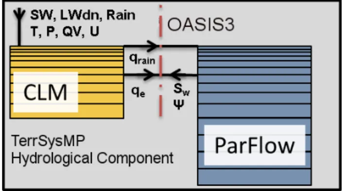
The hydrological component of TerrSysMP consists of the NCAR Community Land Model CLM3.5 (Oleson et al., 2008) and the 3-D variably saturated groundwater and surface water flow code ParFlow (Ashby and Falgout, 1996; Jones and Woodward, 2001; Kollet and Maxwell, 2006; Maxwell, 2013). The two models (Fig. 1) are coupled us-ing the OASIS3 external coupler (Valcke, 2013). In the sequential information exchange procedure, ParFlow sends the updated relative saturation (Sw) and pressure (9) for the top 10 layers to CLM. In turn, CLM sends the depth-differentiated source and sink terms for soil moisture (top soil moisture flux (qrain), soil evapotranspiration (qe)) for the top 10 soil layers to ParFlow (see Fig. 1). A more de-tailed description of the coupling can be found in Shrestha et al. (2014). In this study, the hydrological component of TerrSysMP is decoupled from its atmospheric component and forced with spatially distributed atmospheric forcing data at 2.8 km spatial resolution and hourly temporal resolu-tion (air temperature (T), wind speed (U), specific humidity (QV), total precipitation (Rain), pressure (P), and incoming shortwave (SW) and longwave (LWdn)) from COSMO-DE (Baldauf et al., 2011) analysis data of the German Weather Service (DWD).

Figure 1. Schematic diagram of the hydrological component of the Terrestrial System Modeling Platform (TerrSysMP). OASIS3 is the driver of the component models for land surface (CLM) and sub-surface (ParFlow). The configuration file for OASIS3 prescribes the end-point data exchange between the component models in a se-quential manner. The variables exchanged between the two models are relative saturation (Sw), soil pressure head (9), top soil mois-ture flux (qrain), soil evapotranspiration (qe), air temperature (T), wind speed (U), specific humidity (QV), total precipitation (Rain), pressure (P), and incoming shortwave (SW) and longwave (LWdn).

3 Numerical experiment design

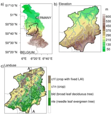
The model was set up for a sub-catchment of the Rur River (TR32 test bed site; Vereecken et al., 2010; Simmer et al., 2014), on the northern foothills of the lower Eifel moun-tain range with an approximated drainage area of 325 km2 (Fig. 2a). The sub-catchment encompasses the tributary We-hebach, which merges with the River Inde. The elevation in the model domain reaches from 50 to 600 m from north to south (Fig. 2b), with mostly agricultural crops (c1n) near the foothills and needleleaf evergreen trees (nle) and broadleaf deciduous trees (bld) along the sloping terrain (Fig. 2c). The urban areas are represented in the model as agricultural canopy (c1f) with a fixed leaf area index (LAI=0.6). Topog-raphy and land use are based on the 90 m resolution Shuttle Radar Topography Mission (SRTM) data and 15 m resolution data available from the TR32 database (Waldhoff, 2012), re-spectively.

(3)

Figure 2. (a) Topography of the Rur catchment, which lies at the border of Germany, Belgium, Luxembourg and the Netherlands. (b) Topography of the sub-catchment of the Rur used in this study (catchment of the River Inde including the Wehebach tributary in the east), overlaid with the stream networks. (c) Land-use map of the sub-catchment.

TerrSysMP with the mosaic approach to better resolve the heterogeneity of topography, land use and geology.

The model setup for all grid resolutions used the same 10 vertically stretched layers (2–100 cm from top to bot-tom) followed by 20 constant depth levels (135 cm) extend-ing to 30 m below the land surface. A uniform soil texture was used for this study by keeping the soil parameters spa-tially constant. The subsurface parameters were set as fol-lows: saturated hydraulic conductivity,Ks=0.00034 m h−1; van Genuchten parameters, α=2.1 and n=2.0 m−1; and porosity,φ=0.4449. This removes any impact of soil het-erogeneity on non-local controls of simulated soil moisture variability and scaling of soil hydraulic properties. The soil moisture profile for all setups was initialized with a hori-zontally homogeneous hydrostatic pressure head and a wa-ter table depth at 5 m from the surface. The soil temperature was also initialized horizontally homogeneous with a uni-form temperature of 10◦C for all levels. A time step of 3600 s was used, and the simulation was integrated for 6 years using hourly atmospheric forcing from COSMO-DE analysis data. The same atmospheric forcing data for the year 2009 were used recursively for the 6 years. The model outputs were av-eraged over 5 days for the analysis. The NCAR Command Language (NCL; NCAR, 2013) was used for data analysis.

Table 1. Model setup indicating the horizontal grid resolution (1X=1Y) and domain discretization.

Model setup 1X=1Y(m) NX×NY×NZ

d120 120 190×220×30

d240 240 100×110×30

d480 480 50×70×30

d960 960 20×30×30

Table 2. Heterogeneity analysis of topography at different grid res-olutions.

Model Plan curvature Profile curvature

domain (m−1) (m−1)

Skewness Kurtosis Skewness Kurtosis

d120 −99.43 13273.9 −0.92 5.66

d240 −2.86 666.28 −0.78 3.97

d480 −8.36 268.06 −0.20 1.92

d960 −0.07 3.64 0.24 0.59

4 Topography heterogeneity analysis

(4)

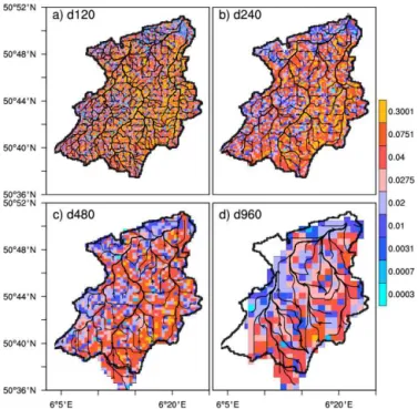
Figure 3. (a–d) Streamlines resulting from D4 flow directions along with slopes for the four grid resolutions. The black solid outline represents the catchment boundary at 120 m resolution.

5 Results and discussions

The simulated unsaturated storage (Sunsat) at different grid resolutions for the sub-catchment showed different temporal evolutions (Fig. 4). The unsaturated storage was normalized by the modeled sub-catchment area to account for differences in catchment size at different grid resolutions. The increase inSunsat during the first year reflects the adjustment of the subsurface storage from the horizontally homogeneous hy-drostatic initial condition, with a ground to water table depth of 5 m. In the first half of this year, the finer grid resolu-tions adjust faster due to a more efficient drainage mecha-nism. In the second year,Sunsatstarts to decrease gradually, reaching a quasi-equilibrium in all simulations in the fifth year. This steady-state value range is lower for the coarser grid resolutions, caused by a higher groundwater table, which results from a less efficient drainage combined with higher infiltration at the lower resolutions. This is also illustrated in Fig. 4b, which shows that the average annual unsaturated storage (Sunsat

t

) in the sixth year is concurrent with the av-erage slope of the sub-catchment. The decrease in avav-erage catchment slope with resolution coarsening is, however, also accompanied by decreasing plan and profile curvature kurto-sis (see Table 2). These results are conkurto-sistent with, e.g., Kuo et al. (1999), who related the increase in average soil mois-ture contents with grid coarsening to decreasing slope gradi-ent and curvature variations. Sulis et al. (2011) also explained catchment wetness in terms of storage and ground to water table depth via decreasing local slopes and plan curvature

Figure 4. (a) Time series of unsaturated storage per unit catch-ment area (Sunsat) for the sub-catchment at the four grid resolutions. (b) Relationship between the annual average unsaturated storage (Sunsatt) and the average catchment slope for the four grid reso-lutions.

variations due to aggregation effects. DifferentSunsat t

with grid resolutions reflects different spatial soil moisture vari-ability, which in turn influences simulated land–atmosphere interactions.

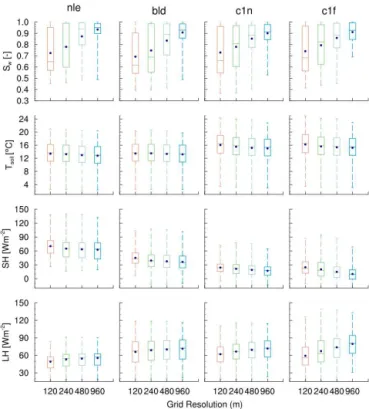
Figure 5 shows the distribution of average top 10 cm rel-ative soil moisture (Sw), average top 10 cm soil temperature (Tsoil), sensible heat flux (SH) and latent heat flux (LH) for time periods when the model exhibits strong coupling with the atmospheric forcing. We assume strong coupling when the 5-day mean incoming solar radiation exceeds 128 Wm−2, which corresponds to the period from April to September. We further filter for different PFTs to analyze the linkages between local vegetation and the non-local controls of soil moisture patterns with grid coarsening. Their respective tem-poral and catchment-averaged values (Sw

x,t ,Tsoil

x,t , SHx,t and LHx,t) are indicated as solid markers (Fig. 5) and sum-marized in Table 3 for the discussion below. For relative soil moisture, grid coarsening leads to a sharp decrease in in-terquartile range and an increase in the 25 % quartile, median and mean value, i.e., reduced variability and higher mean simulated soil moisture. This is true for all PFTs.

(5)

Figure 5. Scaling behavior of relative soil moisture (Sw), soil tem-perature (T_soil), sensible heat flux (SH) and latent heat flux (LH) for the four different canopy covers (nle, bld, c1n and c1f). The solid markers indicate the mean value of the distribution for each grid resolution.

with a fixed low LAI. Average relative soil moisture in-creases by 30 % for trees and 23 % for crops when coars-ening the grid resolution from 120 to 960 m. The difference between the different PFTs is partly related to their spatial location: trees are mostly located in steeper terrain compared to crops (according to the distribution of slopes for the differ-ent PFTs, not shown here). For trees, grid coarsening leads to lowerTsoil

x,t

by 0.6 and 0.3◦C for needleleaf evergreen trees and broadleaf deciduous trees, respectively, while for crops,

Tsoil x,t

is lowered by almost 1◦C. Thus forested grid cells ex-hibit higher grid resolution sensitivity for soil moisture and lower sensitivity for soil temperature, while grid cells with crops show the inverse.

These findings can be attributed to the PFT-specific trans-missivity for solar radiation, or the partitioning of absorbed solar radiation by vegetation and the ground. Needleleaf ev-ergreen trees (nle) absorb more and transmit less solar radi-ation to the ground compared to broadleaf deciduous trees (bld), while the crop type with variable LAI (c1n) absorbs more solar radiation and transmits less compared to the con-stant LAI type (c1f). The PFT-specific optical parameters, in-cluding albedo and amplitudes of seasonal LAI, control the variability in solar radiation partitioning. This directly mod-ulates the partitioning of sensible and latent heat flux and constitutes a local vegetation control.

Table 3. Mean sub-catchment relative soil moisture (Sw), soil tem-perature Tsoil, sensible SHtavg and latent fluxes LHtavg for grid columns with land-use classes nle (needleleaf evergreen tree), bld (broadleaf deciduous tree), c1n (crops with seasonal LAI), and c1f (crops with fixed LAI).

PFT Variable d120 d240 d480 d960

nle

Sw(–) 0.72 0.78 0.87 0.93

Tsoil(◦C) 13.41 13.26 12.97 12.80 SHtavg(Wm−2) 70.3 65.0 63.5 62.6 LHtavg(Wm−2) 49.1 53.0 54.4 55.5

bld

Sw(–) 0.69 0.75 0.83 0.91

c1n

Sw(–) 0.73 0.78 0.85 0.90

c1f

Sw_tavg(–) 0.74 0.79 0.86 0.91

Tsoil_tavg(◦C) 16.22 15.60 15.36 15.20 SHtavg(Wm−2) 25.0 20.3 15.0 10.2 LHtavg(Wm−2) 59.3 67.3 73.8 79.6

For all grid resolutions, the inter-PFT flux differences are much higher than the intra-PFT differences due to differ-ent grid resolutions. In general, grid cells with crops are more sensitive to grid resolution changes. A 60 % decrease in SHx,t and a 35 % increase in LHx,t are observed for c1f, with the grid coarsening from 120 to 960 m. SHx,t decreases by 30 % and LHx,t increases by 16 % for c1n. For forest, SHx,t decreases only by about 20 and 11 %, while LHx,t in-creases only by 8 and 11 % for bld and nle, respectively. In general, the latent heat flux increases and sensible heat flux decreases for all PFTs for coarser grid resolutions, while am-plitudes of change are PFT-dependent, which suggests a lo-cal control by the PFT. This also suggests that the non-lolo-cal control of soil moisture, which is affected by change in grid resolution, also controls the partitioning of surface energy fluxes, especially for PFTs transmitting more solar radiation to the ground. The average relative soil moisture for the sub-catchment in this study was relatively wet; for drier regimes, the effects of model grid resolution on surface fluxes may be stronger.

(6)

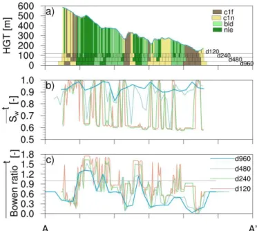
Figure 6. Horizontal variations over cross-section AA′ in Fig. 2: (a) topography and land use, (b) annual average top 10 cm relative soil moisture and (c) annual average Bowen ratio at different model grid resolutions.

along cross-section AA′_{indicated in Fig. 2 for different grid}

resolutions. The difference in variability of topography is not visible along the cross section due to the plot scale, but the effect of grid resolution on the simulated average top 10 cm soil moistureSw

t

is obvious in Fig. 6b. With grid coarsening, the finer scale plan and profile curvatures are filtered, which reduces drainage efficiency, increases the simulated grid cell soil moisture, and damps the spatial variability. This effect is more pronounced from d240 to d480 and d960 than from d120 to d240. Quantitatively, the spatial average and standard deviation forSw

t

along the cross-section AA′are 0.70±0.16, 0.75±0.17, 0.90±0.10 and 0.93±0.04 for d120, d240, d480 and d960, respectively, which clearly shows the increase in soil wetness and decrease in variability with coarsening with largest changes between d240 and d480.

The strong scaling behavior of soil moisture also mod-ulates the partitioning of surface energy fluxes. Figure 6c shows the annual average Bowen ratio (ratio of sensible to latent heat flux) along cross-section AA′; its profile matches well with the PFT profile, indicating local vegetation con-trol on the spatial pattern of surface flux partitioning. This could be partly enhanced due to the wet soil condition in the sub-catchment for the simulated period. However, the change in the non-local control of soil moisture with grid resolution also contributes to the profile of surface flux partitioning vis-ible as a perturbation in the amplitudes of the Bowen ratio for d960. Some perturbations are also caused by different PFTs for finer grid resolution. Table 4 summarizes the statistics of the Bowen ratio profile along the cross section and shows

Table 4. Annual average Bowen ratio and standard deviation along the cross-section AA′for the land-use classes nle (needleleaf ever-green tree), bld (broadleaf deciduous tree), c1n (crops with seasonal LAI), and c1f (crops with fixed LAI).

PFT 120 m 240 m 480 m 960 m

nle 1.56±0.16 1.35±0.22 1.22±0.12 1.24±0.07 bld 0.82±0.08 0.72±0.08 0.60±0.09 0.59±0.08 c1n 0.46±0.13 0.50±0.15 0.36±0.13 0.28±0.07 c1f 0.67±0.28 0.53±0.38 0.17±0.11 0.18±0.13

that its dominant pattern is strongly controlled by the PFT pattern. For trees, nle has a higher Bowen ratio (>1) than bld (<1), which is mainly due to differences in plant phys-iological properties, consistent with observations (Baldocchi et al., 1997). For crops, c1f has a higher Bowen ratio com-pared to c1n, which is due to the LAI difference. For both trees and crops, the Bowen ratio in general decreases with grid coarsening. Coarsening from d120 to d960 decreases the Bowen ratio by 20, 28, 39, and 73 % for nle, bld, c1n and c1f, respectively. The most significant change is found for crops with low LAI. Radiation absorbed by the ground plays a significant role in amplifying/attenuating the grid resolu-tion dependence of surface flux partiresolu-tioning. Again, it has to be mentioned that this statement may be valid only for wet regimes.

Figure 7 shows the scatterplot between the Bowen ratio and average top 10 cm relative soil moisture along cross-section AA′ over the averaged time period filtered for dif-ferent PFTs to illustrate the PFT-related dependence of the Bowen ratio on relative soil moisture. Large scatter for d480 and d960 m is found forSw<0.7, while for d120 and d240, large scatter is only found forSw≤0.4. Thus, the Bowen ra-tio distribura-tion shifts with grid resolura-tion. A linear regression between Bowen ratio and relative soil moisture gives a first-order estimate of the Bowen ratio dependence on relative soil moisture. Tree canopies exhibit more variability in the Bowen ratio than crops. For trees, nle exhibits stronger scal-ing behavior with relative soil moisture than bld. For crops, c1f exhibits stronger scaling behavior with relative soil mois-ture than c1n. The results again show that crops with low LAI have a stronger influence on flux partitioning with grid reso-lution.

(7)

Figure 7. Distribution of the Bowen ratio as a function of relative soil moisture along cross-section AA′. The distribution is plotted separately for different land-use types in the sub-catchment.

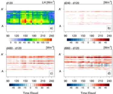
strength would also depend on the mean heating rates of the catchment and the synoptic wind strength as indicated in many previous studies (Lemone et al., 2002; Baidya Roy and Avissar, 2002; Grossman et al., 2005). Figure 8b–d shows the difference in the time series of SH along cross-section AA′ _{between the coarser grid resolutions and d120. With}

grid coarsening the amplitude of the SH difference increases, suggesting an overall decrease in SH as also observed from the bulk quantities. Some d960 grid cells also exhibit an increase in SH mainly due to the changing dominant PFT, when the subgrid cells consist of trees and crops. Similarly, Fig. 9a shows the time series of 5-day average latent heat flux along cross-section AA′for d120, which also exhibits a strong seasonal cycle and a strong gradient along AA′. The difference in time series of LH along AA′for coarser resolu-tions with respect to d120 shows the sharp increase in latent heat flux. The decrease and increase in SH and LH, respec-tively, are particularly high between 480 and 960 m resolu-tion. Thus, when using coarser grid resolutions for the hydro-logical model, coupled to the atmospheric model, the simu-lated boundary layer would be relatively moister and cooler.

6 Summary and conclusions

This study was motivated by recent efforts in including phys-ically based hydrological models in earth system models both for seasonal-scale and climate studies that would allow

Figure 8. (a) Time evolution of 5-day mean sensible heat flux (SH) along cross-section AA′for the d120 domain. (b) Difference in the time evolution of SH between the d240 and d120. (c) Difference in the time evolution of SH between the d480 and d120. (d) Difference in the time evolution of SH between the d960 and d120. For d120, d240 and d480, the SH fluxes were spatially aggregated to 960 m resolution.

Figure 9. (a) Time evolution of 5-day mean sensible heat flux (LH) along cross-section AA′for the d120 domain. (b) Difference in the time evolution of LH between the d240 and d120. (c) Difference in the time evolution of LH between the d480 and d120. (d) Difference in the time evolution of LH between the d960 and d120. For d120, d240 and d480, the LH fluxes were spatially aggregated to 960 m resolution.

(8)

sub-catchment of the Rur at grid resolutions encompassing roughly the spatial scales between LES and mesoscale atmo-spheric models to quantify the effect of grid resolution on simulated soil moisture, soil temperature and surface fluxes. The terrain analysis of the sub-catchment showed the ex-pected smoothing of slopes and filtering of the profile and plan curvatures with grid coarsening. This grid resolution has a strong effect on the non-local controls of soil mois-ture simulated by the model, while the local vegetation exerts a strong modulation on the transfer of the grid-resolution-dependent soil moisture variability to soil temperature and surface fluxes. In this study, soil moisture beneath forests was found to decrease more than beneath crops due to the location of forests over steeper slopes. However, due to the plant physiological properties affecting the transmissivity of solar radiation, crops lead to a higher grid resolution depen-dence than trees in terms of soil temperature and surface fluxes. For crops, the magnitude of the LAI was also found to have a strong effect on the scaling behavior of surface fluxes. This non-linear scaling behavior of the energy balance with respect to grid resolution can alter the spatial and tem-poral pattern of simulated surface fluxes. Larger differences were especially observed when moving from d480 to d960. These dependencies can induce or weaken mesoscale circu-lations and the ensuing boundary layer evolution when using coupled simulations. Using an idealized setup, such atmo-spheric feedback effects for a rainfall–runoff process (runoff due to excess infiltration, creating wet and dry patches), with varying grid resolution, were shown earlier by Shrestha et al. (2014). Here the heterogeneity at different resolutions was introduced in terms of topographic slopes while keep-ing a homogeneous land cover (crop). In this study, the in-clusion of convergent zones at finer grid resolutions com-pared to coarser grid resolutions, where they are usually filtered out by topography smoothing, enhanced the over-land flow, thereby reducing the infiltration and the mean soil moisture content while extending the downslope moist area. This extended downslope moist area increased the extent of the moist patch compared to the coarser run, thereby low-ering the Bowen ratio along the extended patch, and also increasing the extent of the downdraft region in the atmo-spheric boundary layer. Thus, the dependence of the simu-lated surface–subsurface physical processes on grid resolu-tion potentially also affects the local circularesolu-tion and atmo-spheric boundary layer evolution. However, fully coupled real data simulations including the atmosphere at different grid resolutions are required to further improve our under-standing of the land–atmosphere feedbacks.

The study was limited to grid resolutions from 120 to 960 m. One could argue that even the 120 m resolution is not sufficient for hydrological models, and much finer res-olutions (≤30 m) are needed (e.g., Kuo et al., 1999). We ac-knowledge the limitation in this study, but finer resolutions challenge currently available computation resources and also the convergence of 3-D integrated surface groundwater

mod-els. We realize that sub-grid-scale parameterizations along with resolutions of approximately 100–200 m would be suf-ficient for coupled simulations. The interaction between sur-face and groundwater in ParFlow is simulated using a 2-D shallow overland flow equation as an upper boundary condi-tion (Kollet and Maxwell, 2006), instead of the commonly applied conductance concept. Particularly for the surface– groundwater interaction, this upper boundary condition and the Darcy flux in the horizontal direction are affected by the spatial filtering of the terrain curvature in the coarsening of the grid resolution. This results in an increase in infiltration, a reduction of lateral flow and a shallower groundwater table. So, there is a need for a scale-dependent subgrid parameter-ization for the upper boundary condition and for the lateral flow in the groundwater model used in this study. For the upper boundary condition, e.g., the concept of a fractional saturated area (parameterized by the subgrid-scale distribu-tions of topographic index and groundwater table depth) is widely used to control surface runoff and hence infiltration in many 1-D land surface models (e.g., Niu et al., 2005). For the subsurface, e.g., Niedda (2004) proposed an amplifica-tion/upscaling of hydraulic conductivity to compensate for the reduction in the hydraulic gradients using the information content of terrain curvature to produce similar lateral flow. In general, the topography heterogeneity analysis and the soil moisture data presented in this study do provide the neces-sary data to investigate such parameterizations for the upper boundary condition and lateral subsurface flow. Future stud-ies will involve developing such robust scale-dependent sub-grid parameterization for the 3-D physically based ground-water model.

Acknowledgements. This study was conducted with support from SFB/TR32 (www.tr32.de), “Patterns in Soil-Vegetation-Atmosphere Systems: Monitoring, Modelling, and Data Assimi-lation”, funded by the Deutsche Forschungsgemeinschaft (DFG). We thank the Deutscher Wetterdienst (DWD) for the COSMO analysis data. The data analysis including the pre-processing and post-processing of input data for TerrSysMP was done using the NCAR Command language (version 6.2.0).

Edited by: I. Neuweiler

References

Anyah, R. O., Weaver, C. P., Miguez-Macho, G., Fan, Y., and Robock, A.: Incorporating water table dynamics in climate modeling: 3. Simulated groundwater influence on coupled land–atmosphere variability, J. Geophys. Res., 113, D07103, doi:10.1029/2007JD009087, 2008.

Ashby, S. F. and Falgout, R. D.: A parallel multigrid preconditioned conjugate gradient algorithm for groundwater flow simulations, Nucl. Sci. Eng., 124, 145–159, 1996.

(9)

bound-ary layer using large-eddy simulations, J. Atmos. Sci., 55, 2666– 2689, 1998.

Baidya Roy, S. and Avissar, R.: Impact of land use/land cover change on regional hydrometeorology in Amazonia, J. Geophys. Res., 107, LBA 4-1–LBA 4-12, doi:10.1029/2000JD000266, 2002.

Baldauf, M., Seifert, A., Förstner, J., Majewski, D., Raschendor-fer, M., and Reinhardt, T.: Operational convective-scale nu-merical weather prediction with the COSMO model: descrip-tion and sensitivities, Mon. Weather Rev., 139, 3887–3905, doi:10.1175/MWR-D-10-05013.1, 2011.

Baldocchi, D. D., Vogel, C. A., and Hall, B.: Seasonal variation of carbon dioxide exchange rates above and below a boreal jack pine forest, Agr. Forest Meteorol., 83, 147–170, 1997.

Becker, A. and Braun, P.: Disaggregation, aggregation and spa-tial scaling in hydrological modelling, J. Hydrol., 217, 239–252, 1999.

Beven, K. J. and Cloke, H. L.: Comment on “Hyperresolution global land surface modeling: meeting a grand challenge for monitoring Earth’s terrestrial water” by Eric F. Wood et al., Water Resour. Res., 48, W01801, doi:10.1029/2011WR010982, 2012. Blöschl, G. and Sivapalan, M.: Scale issues in hydrological

mod-elling: a review, Hydrol. Process., 9, 251–290, 1995.

Bormann, H.: Impact of spatial data resolution on simulated catch-ment water balances and model performance of the multi-scale TOPLATS model, Hydrol. Earth Syst. Sci., 10, 165–179, doi:10.5194/hess-10-165-2006, 2006.

Butts, M., Drews, M., Larsen, M. A., Lerer, S., Rasmussen, S. H., Grooss, J., Overgaard, J., Refsgaard, J. C., Christensen, O. B., and Christensen, J. H.: Embedding complex hydrology in the re-gional climate system-dynamic coupling across different mod-elling domains, Adv. Water Resour., 74, 166–184, 2014. Cai, X. and Wang, D.: Spatial autocorrelation of topographic index

in catchments, J. Hydrol., 328, 581–591, 2006.

Dixon, B. and Earls, J.: Resample or not?! Effects of resolution of DEMs in watershed modeling, Hydrol. Process., 23, 1714–1724, 2009.

Gasper, F., Goergen, K., Shrestha, P., Sulis, M., Rihani, J., Geimer, M., and Kollet, S.: Implementation and scaling of the fully cou-pled Terrestrial Systems Modeling Platform (TerrSysMP v1.0) in a massively parallel supercomputing environment – a case study on JUQUEEN (IBM Blue Gene/Q), Geosci. Model Dev., 7, 2531–2543, doi:10.5194/gmd-7-2531-2014, 2014.

Giertz, S., Diekkrüger, B., and Steup, G.: Physically-based modelling of hydrological processes in a tropical headwater catchment (West Africa) – process representation and multi-criteria validation, Hydrol. Earth Syst. Sci., 10, 829–847, doi:10.5194/hess-10-829-2006, 2006.

Grayson, R. B., Western, A. W., Chiew, F. H., and Blöschl, G.: Pre-ferred states in spatial soil moisture patterns: local and nonlocal controls, Water Resour. Res., 33, 2897–2908, 1997.

Grossman, R. L., Yates, D., LeMone, M. A., Wesely, M. L., and Song, J.: Observed effects of horizontal radiative surface temperature variations on the atmosphere over a Midwest wa-tershed during CASES 97, J. Geophys. Res., 110, D06117, doi:10.1029/2004JD004542, 2005.

Herbst, M., Diekkrueger, B., and Vanderborght, J.: Numerical ex-periments on the sensitivity of runoff generation to the spatial

variation of soil hydraulic properties, J. Hydrol., 326, 43–58, 2006.

Jones, J. E. and Woodward, C. S.: Newton-krylov-multigrid solvers for large-scale, highly heterogeneous, variably saturated flow problems, Adv. Water Resour., 24, 763–774, 2001.

Kollet, S. J. and Maxwell, R. M.: Integrated surface–groundwater flow modeling: a free-surface overland flow boundary condition in a parallel groundwater flow model, Adv. Water Ressour., 29, 945–958, 2006.

Kuo, W. L., Steenhuis, T. S., McCulloch, C. E., Mohler, C. L., We-instein, D. A., DeGloria, S. D., and Swaney, D. P.: Effect of grid size on runoff and soil moisture for a variable-source-area hy-drology model, Water Resour. Res., 35, 3419–3428, 1999. Larsen, M. A. D., Refsgaard, J. C., Drews, M., Butts, M. B., Jensen,

K. H., Christensen, J. H., and Christensen, O. B.: Results from a full coupling of the HIRHAM regional climate model and the MIKE SHE hydrological model for a Danish catchment, Hy-drol. Earth Syst. Sci., 18, 4733–4749, doi:10.5194/hess-18-4733-2014, 2014.

LeMone, M. A., Grossman, R. L., Mcmillen, R. T., Liou, K. N., Ou, S. C., Mckeen, S., Angevine, W., Ikeda, K., and Chen, F.: CASES-97: late-morning warming and moistening of the con-vective boundary layer over the Walnut River watershed, Bound.-Lay. Meteorol., 104, 1–52, 2002.

Maxwell, R. M.: A terrain-following grid transform and precondi-tioner for parallel, large-scale, integrated hydrologic modeling, Adv. Water Resour., 53, 109–117, 2013.

Maxwell, R. M., Lundquist, J. K., Mirocha, J. D., Smith, S. G., Woodward, C. S., and Tompson, A. F.: Development of a Cou-pled Groundwater–Atmosphere Model, Mon. Weather Rev., 139, 96–116, doi:10.1175/2010MWR3392.1, 2011.

Niedda, M.: Upscaling hydraulic conductivity by means of en-tropy of terrain curvature representation, Water Resour. Res., 40, W04206, doi:10.1029/2003WR002721, 2004.

Niu, G. Y., Yang, Z. L., Dickinson, R. E., and Gulden, L. E.: A simple TOPMODEL-based runoff parameterization (SIMTOP) for use in global climate models, J. Geophys. Res., 110, D21106, doi:10.1029/2005JD006111, 2005.

Oleson, K. W., Niu, G. Y., Yang, Z. L., Lawrence, D. M., Thornton, P. E., Lawrence, P. J., Stöckli, R., Dickinson, R. E., Bonan, G. B., Levis, S., Dai, A., and Qian, T.: Improvements to the Community Land Model and theirimpact on the hydrological cycle, J. Geo-phys. Res., 113, G01021, doi:10.1029/2007JG000563, 2008. Quinn, P. F., Beven, K. J., and Lamb, R.: The in (a/tan/β) index:

how to calculate it and how to use it within the topmodel frame-work, Hydrol. Process., 9, 161–182, 1995.

Sciuto, G. and Diekkrueger, B.: Influence of soil heterogeneity and spatial discretization on catchment water balance modeling, Va-dose Zone J., 9, 955–969, 2010.

Shrestha, P., Sulis, M., Masbou, M., Kollet, S., and Simmer, C.: A scale-consistent terrestrial systems modeling platform based on COSMO, CLM, and Parflow, Mon. Weather Rev., 142, 3466– 3483, 2014.

(10)

G.: Monitoring and modeling the terrestrial system from pores to catchments – the transregional collaborative research center on Patterns in the soil-vegetation-atmosphere system, B. Am. Mete-orol. Soc., doi:10.1175/BAMS-D-13-00134.1, online first, 2014. Sulis, M., Paniconi, C., and Camporese, M.: Impact of grid res-olution on the integrated and distributed response of a cou-pled surface–subsurface hydrological model for the des Anglais catchment, Quebec, Hydrol. Process., 25, 1853–1865, 2011. Sulis, M., Langensiepen, M., Shrestha, P., Schickling, A.,

Sim-mer, C., and Kollet, S. J.: Evaluating the influence of plant-specific physiological parameterizations on the partitioning of land surface energy fluxes, J. Hydrometeorol., 16, 517–533, doi:10.1175/JHM-D-14-0153.1, 2015.

The NCAR Command Language: Version 6.1.2 (Soft-ware), UCAR/NCAR/CISL/VETS, Boulder, Colorado, doi:10.5065/D6WD3XH5, 2013.

Valcke, S.: The OASIS3 coupler: a European climate mod-elling community software, Geosci. Model Dev., 6, 373–388, doi:10.5194/gmd-6-373-2013, 2013.

Vereecken, H., Kollet, S., and Simmer, C.: Patterns in soil-vegetation-atmosphere systems: monitoring, model-ing, and data assimilation, Vadose Zone J., 9, 821–827, doi:10.2136/vzj2010.0122, 2010.

Vivoni, E. R., Ivanov, V. Y., Bras, R. L., and Entekhabi, D.: On the effects of triangulated terrain resolution on distributed hydro-logic model response, Hydrol. Process., 19, 2101–2122, 2005. Waldhoff, G.: Enhanced Land Use Classification of 2009

for the Rur catchment, CRC/TR32 Database (TR32DB), doi:10.5880/TR32DB.2, 2012.

Wood, E. F., Roundy, J. K., Troy, T. J., van Beek, L. P. H., Bierkens, M. F. P., Blyth, E., de Roo, A., Döll, P., Ek, M., Famiglietti, J., Gochis, D., van de Giesen, N., Houser, P., Jaffé, P. R., Kol-let, S., Lehner, B., Lettenmaier, D. P., Peters-Lidard, C., Siva-palan, M., Sheffield, J., Wade, A., and Whitehead, P.: Hyperres-olution global land surface modeling: meeting a grand challenge for monitoring Earth’s terrestrial water, Water Resour. Res., 47, W05301, doi:10.1029/2010WR010090, 2011.