Brief Communication "Importance of slope-induced error correction in elevation change estimates from radar altimetry"

(1)

TCD

6, 159–170, 2012

Importance of slope-induced error

correction

R. T. W. L. Hurkmans et al.

Title Page

Abstract Introduction

Conclusions References

Tables Figures

◭ ◮

Back Close

Full Screen / Esc

Printer-friendly Version Interactive Discussion

Discussion

P

a

per

|

Dis

cussion

P

a

per

|

Discussion

P

a

per

|

Discussio

n

P

a

per

|

The Cryosphere Discuss., 6, 159–170, 2012 www.the-cryosphere-discuss.net/6/159/2012/ doi:10.5194/tcd-6-159-2012

The Cryosphere Discussions

This discussion paper is/has been under review for the journal The Cryosphere (TC). Please refer to the corresponding final paper in TC if available.

Brief Communication

“Importance of slope-induced error

correction in elevation change estimates

from radar altimetry”

R. T. W. L. Hurkmans, J. L. Bamber, and J. A. Griggs

Bristol Glaciology Centre, School of Geographical Sciences, University of Bristol, Bristol, UK

Received: 16 December 2011 – Accepted: 10 January 2012 – Published: 17 January 2012

Correspondence to: R. T. W. L. Hurkmans (ruud.hurkmans@bristol.ac.uk)

(2)

TCD

6, 159–170, 2012

correction

Title Page

Tables Figures

◭ ◮

Back Close

Full Screen / Esc

Discussion

P

a

per

|

Dis

cussion

P

a

per

|

Discussion

P

a

per

|

Discussio

n

P

a

per

|

Abstract

In deriving elevation change rates (dH/dt) from radar altimetry, the slope-induced error is usually assumed to cancel out in repeat measurements. These measurements, however, represent a location that can be significantly further upslope than assumed, causing an underestimate of the basin-integrated volume change. In a case-study for

5

the fast-flowing part of Jakobshavn Isbræ, we show that a relatively straightforward correction for slope-induced error increases elevation change rates by several metres and increases the volume change by 32 % for the region of interest.

1 Introduction

Several sources of uncertainty affect measurements of ice sheet surface elevation

de-10

rived from satellite radar altimetry (SRA; e.g. Brenner et al., 2007; Bamber, 1994). Po-tentially the largest one, referred to as the slope-induced error (Brenner et al., 1983), is caused by regional surface slopes. For narrow, fast-flowing outlet glaciers, the low-est surface may not be sampled at all (see Fig. 9 of Thomas et al., 2008), however these are often the areas that show the largest elevation changes (Pritchard et al.,

15

2009). The radar return signal does not originate from the point directly underneath the satellite (nadir), but from the closest point to the satellite, which can be significantly displaced upslope from nadir. For a 1◦ slope, which is not unusual at the ice sheet margin, the displacement between nadir and the actual measurement location is about 14 km, and the vertical error is about 120 m. Using a regional slope estimate, it is

20

relatively straightforward to relocate the measurement to its correct location (Bamber, 1994). When elevationchange is concerned, however, it is usually assumed that the slope-induced error remains constant and the e_ffect cancels (Thomas et al., 2008). While the error in the vertical is indeed the same for repeating elevation measure-ments, the location of the measured elevation change rate will still be displaced from

25

(3)

TCD

6, 159–170, 2012

correction

Title Page

Tables Figures

◭ ◮

Back Close

Full Screen / Esc

Discussion

P

a

per

|

Dis

cussion

P

a

per

|

Discussion

P

a

per

|

Discussio

n

P

a

per

|

underestimated, because elevation changes that are measured at an upslope location are incorrectly located closer to the margin.

2 Data

To demonstrate the effect of correcting for slope-induced error, we use data from the radar altimeter (RA-2) on ESA’s Envisat satellite, that was launched in 2002. It

con-5

tinues the SRA time series from ERS-1 and ERS-2 and is in a similar orbit with an altitude of about 800 km, a repeat period of 35 days, and a latitudinal coverage up to 81.5◦_{. We used Envisat cross-over clusters (Li and Davis, 2008) from which average}

elevation change rates for 2003–2006 were derived. The selected study area is the fast-flowing region of Jakobshavn Isbræ, Greenland’s largest outlet glacier, located on

10

the Southwest coast. Since about 1998, it has been accelerating and thinning signifi-cantly (Joughin et al., 2008), and has been densely surveyed by airborne laser altimetry (ATM; Krabill et al., 2004).

We use airborne (ATM) and spaceborne (ICESat) laser altimetry data as a validation data set. Elevations from these data sources do not suffer from slope-induced error as

15

they have a small footprint with known pointing: ≈60 m for ICESat (Zwally et al., 2002)

and 1–2 m for ATM (Krabill et al., 2002). Elevation change rates for 2003–2006 (con-sistent with Envisat) were derived from ICESat using the “plane” method (Howat et al., 2008). A plane is fitted through data from several near-repeat tracks. For each plane, which is typically about 700 m long and a few hundreds of metres wide, two-directional

20

slopes and a temporal elevation change ratedH/dt are fitted using multivariate linear regression (Moholdt et al., 2010). A regression is only performed if a plane has at least 10 points from four different tracks that span at least a year. Prior to the regres-sion, outliers (outside 2σ) are removed, and only elevation changes with an associated standard error ondH/dt of less than 0.50 m yr−1 are considered. ATM footprints were

25

(4)

TCD

6, 159–170, 2012

correction

Title Page

Tables Figures

◭ ◮

Back Close

Full Screen / Esc

Discussion

P

a

per

|

Dis

cussion

P

a

per

|

Discussion

P

a

per

|

Discussio

n

P

a

per

|

elevation change rates from all available flight lines, but instead of platelets, 1 km pix-els were used.

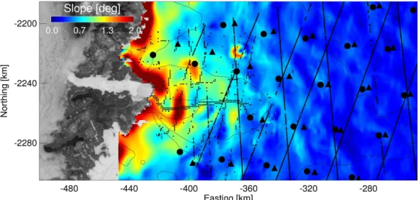
Other datasets that are employed here are a 1 km digital elevation model (Bamber et al., 2001) from which slope and aspect are derived, and an ice sheet velocity mosaic used for interpolation. The velocity field was derived from a combination of radar

inter-5

ferometry and speckle tracking using RADARSAT-2 data from the winters 2000–2001, 2005–2006, and 2007–2008 (Joughin et al., 2010). Figure 1 shows the slope, as well as locations of Envisat cross-over points, ICESat tracks, ATM flight lines, and velocity contours for the fast-flowing part of Jakobshavn Isbræ.

3 Methodology

10

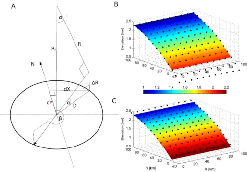
The slope-induced error is schematically illustrated in Fig. 2a by a range measurement

R to an inclined surface with slopeαand aspect β. The measurement location is dis-placed from nadir by a horizontal distanceD. Three correction methods for the range exist (Bamber, 1994). First, the direct method corrects the range measured at nadir (corrected rangeRc=R/cos(α)). The second method, the relocation method, corrects

15

R toRc: the closest point to the satellite (nowRcos(α)), and displaces the location by

Rsin(α). The intermediate method, finally, finds the location where R=Rc, and relo-cates the measurement to that point (Remy et al., 1989). When one is interested in elevationchanges, errors in the vertical cancel out, but measurements are still located at the wrong locations. This can lead to underestimation of area-integrated volume

20

changes asdH/dt values obtained by radar altimetry are actually located further ups-lope than assumed (Fig. 2). For cross-over analyses, wheredH/dt is derived for loca-tions where ascending and descending tracks cross each other, a two-dimensional cor-rection should be applied. The displacementDis given byD=Esin(α)cos(α), whereE

is the satellite altitude, equivalent toRcin Fig. 2a, and 800±20 km for Envisat.

Sensitiv-25

ity to variations in the orbit altitude is small: a sensitivity experiment indicated that, at 1◦

(5)

TCD

6, 159–170, 2012

correction

Title Page

Tables Figures

◭ ◮

Back Close

Full Screen / Esc

Discussion

P

a

per

|

Dis

cussion

P

a

per

|

Discussion

P

a

per

|

Discussio

n

P

a

per

|

with respect to the displacement for an altitude of 800 km. Sensitivity to slope angle is larger (e.g. an increase of 0.1◦ causes a≈10 % change in horizontal displacement);

it is therefore important to use contemporaneous estimates of slope. The direction of displacement is opposite to the slope aspect β, which is the direction of the steep-est downward slope. If β is defined as 0 radians for north and increasing clockwise

5

to 2π radians, the relocation in x and y directions are given byd X =Dsin(β−π) and

d Y =Dcos(β−π). Although small-scale undulations can also cause error (Bamber and

Gomez-Dans, 2005), we use average slope and aspect over a 100 km2area centered on the cross-over location to correct for regional slope, as 10 km is the approximate length scale of the expected displacement.

10

We illustrate the e_ffect of the correction on volume change using a hypothetical test-case. We simulated a 100×100 km surface with a slope increasing linearly toward

lower elevations from 0.5 to 1.5◦ (Fig. 2b). SyntheticdH/dt data, ranging linearly from 2 m yr−1

at 1.5◦ _{slope to 1 m yr}−1

at 0.5◦ _{slope, are evenly spaced at 10 km intervals.}

dH/dt data coverage is assumed to extend linearly beyond the domain, so the

correc-15

tion displaces data points “into” the domain. A full 1 km resolution dH/dt field is ob-tained using inverse distance interpolation. In Fig. 2c, all data locations are corrected for slope-induced error, enlarging the area with the largestdH/dt. For this particular test case, the relative difference in volume change (i.e., between Fig. 2b and c) is 10.4 %. It should be noted that dH/dt values are relatively modest compared to Jakobshavn

20

Isbræ.

4 Results

Figure 3a shows a scatterplot ofdH/dt from Envisat cross-over clusters versusdH/dt

from interpolation of ATM/ICESat, for both the uncorrected and the corrected Envisat locations. Interpolation was conducted using kriging with external drift (KED), which

25

(6)

TCD

6, 159–170, 2012

correction

Title Page

Tables Figures

◭ ◮

Back Close

Full Screen / Esc

Discussion

P

a

per

|

Dis

cussion

P

a

per

|

Discussion

P

a

per

|

Discussio

n

P

a

per

|

dH/dt measurements. The method is described in detail elsewhere (Hurkmans et al., 2012), where they found that for Jakobshavn Isbræ, KED results in more realisticdH/dt

patterns (with respect to ATM) than other methods investigated. The sparsity of En-visat data is illustrated by the fact that there are only 23 EnEn-visat cross-over clusters in the study area. “Outliers” present in the uncorrected values are generally corrected

to-5

wards the ATM/ICESat values effectively, sometimes with elevation corrections of sev-eral metres. There is still, however, considerable noise in the corrected data, because (i) the correction only corrects for the footprint-average slope and not for smaller scale undulations, and (ii) interpolated values from ATM/ICESat were used because Envisat and ATM/ICESat footprints never exactly overlap. The effectiveness of the correction

10

is illustrated by the correlation coe_fficient which increases from 0.35 to 0.88 after the correction for slope-induced error.

InterpolateddH/dt values are shown in Fig. 3b and c. In Fig. 3b, a transect is shown constructed by calculating the average north-southdH/dt within the 300 m yr−1

velocity contour for each 1 km pixel moving east from the grounding zone. The difference in

15

thinning rates between corrected and uncorrected Envisat data increases from about 0.4 m yr−1

at 80 km from the grounding zone to about 4 m yr−1

at 10 km. A three kilome-tre zone adjacent to the presumed grounding line was not taken into account because of uncertainty in its location (Hurkmans et al., 2012), hence dH/dt values increase close to the grounding line. After correction for slope-induced error, interpolated

thin-20

ning rates are both larger and more widespread. This can be seen in Fig. 3c, where the difference between interpolateddH/dt values with and without slope-correction are shown. The e_ffect of the correction can also be quantified by calculating the inte-grated volume change for the area. The volume change for the area enclosed by the 100 m yr−1 velocity contour is 8.6 km3yr−1 for uncorrected Envisat and 11.4 km3yr−1

25

(7)

TCD

6, 159–170, 2012

correction

Title Page

Tables Figures

◭ ◮

Back Close

Full Screen / Esc

Discussion

P

a

per

|

Dis

cussion

P

a

per

|

Discussion

P

a

per

|

Discussio

n

P

a

per

|

5 Conclusions

In deriving volume change estimates over the ice sheets, and from these mass change, from satellite radar altimetry, the effect of slope-induced error on thedH/dt location is usually ignored because the vertical error cancels out in repeat measurements. The estimateddH/dt values are, however, representative of locations further upslope than

5

assumed, resulting in an underestimate of the volume change, and the elevation rate at the sub-satellite location. We show that this underestimation is substantial for an outlet glacier such as Jakobshavn Isbræ, where slopes can be up to 2◦. For the fast flowing section of the catchment (where the density of the volume change is approximately that of ice) the di_fference in volume change was 32 %. Correcting for slope-induced error

10

is a relatively straightforward procedure, but is important in deriving accurate ice sheet mass loss from ice sheets.

Acknowledgements. This work was supported by funding to the ice2sea programme from the European Union 7th Framework Programme, grant number 226375. Ice2sea contribution num-ber 69. JAG was funded by the European Space Agency’s Changing Earth Science net-15

work. We also thank C. Davis (University of Missouri), W. Krabill (NASA GSFC), L. Sandberg-Sørensen (DTU Space, Copenhagen) and I. Joughin (University of Washington) for allowing access to their data.

References

Bamber, J. L.: Ice sheet altimeter processing scheme, Int. J. Remote Sens., 15, 925–938, 20

doi:10.1080/01431169408954125, 1994. 160, 162

Bamber, J. and Gomez-Dans, J. L.: The accuracy of digital elevation models of the Antarctic continent, Earth Planet. Sc. Lett., 237, 516–523, doi:10.1016/j.epsl.2005.06.008, 2005. 163 Bamber, J. L., Ekholm, S., and Krabill, W. B.: A new, high-resolution digital elevation model of Greenland fully validated with airborne laser altimeter data, J. Geophys. Res., 106, 6733– 25

(8)

TCD

6, 159–170, 2012

correction

Title Page

Tables Figures

◭ ◮

Back Close

Full Screen / Esc

Discussion

P

a

per

|

Dis

cussion

P

a

per

|

Discussion

P

a

per

|

Discussio

n

P

a

per

|

Brenner, A. C., Bindschadler, R. A., Thomas, R. H., and Zwally, H. J.: Slope-induced errors in radar altimetry over continental ice sheets, J. Geophys. Res., 88, 1617–1623, 1983. 160 Brenner, A. C., DiMarzio, J. P., and Zwally, H. J.: Precision and accuracy of satellite radar and

laser altimeter data over the continental ice sheets, IEEE T. Geosci. Remote., 45, 321–331, doi:10.1109/TGRS.2006.887172, 2007. 160

5

Howat, I. M., Smith, B. E., Joughin, I., and Scambos, T. E.: Rates of southeast Greenland ice volume loss from combined ICESat and ASTER observations, Geophys. Res. Lett., 35, L17505, doi:10.1029/2008GL034496, 2008. 161

Hurkmans, R. T. W. L., Bamber, J. L., Sørensen, L. S., Joughin, I., Davis, C. H., and Krabill, W.: Spatio-temporal interpolation of elevation changes derived from satellite altimetry for Jakob-10

shavn Isbræ, Greenland, J. Geophys. Res., in review, 2012. 164

Joughin, I., Howat, I. M., Fahnestock, M., Smith, B., Krabill, W., Alley, R. B., Stern, H., and Tru_ffer, M.: Continued evolution of Jakobshavn Isbræ following its rapid speedup, J. Geophys. Res., 113, F04006, doi:10.1029/2008JF001023, 2008. 161

Joughin, I., Smith, B. E., Howat, I. M., Scambos, T., and Moon, T.: Greenland flow variability 15

from ice-sheet-wide velocity mapping, J. Glaciol., 56, 415–430, 2010. 162

Krabill, W. B., Abdalati, W., Frederick, E. B., Manizade, S. S., Martin, C. F., Sonntag, J. G., Swift, R. N., Thomas, R. H., and Yungel, J. G.: Aircraft laser altimetry measurement of eleva-tion changes of the Greenland ice sheet: technique and accuracy assessment, J. Geodyn., 34, 357–376, 2002. 161

20

Krabill, W., Hanna, E., Huybrechts, P., Abdalati, W., Cappelen, J., Csatho, B., Freder-ick, E., Manizade, S., Martin, C., Sonntag, J., Swift, R., Thomas, R., and Yungel, J.: Greenland ice sheet: increased coastal thinning, Geophys. Res. Lett., 31, L24402, doi:10.1029/2004GL021533, 2004. 161

Li, Y. and Davis, C. H.: Decadal mass balance of the Greenland and Antarctic ice sheets from 25

high resolution elevation change analysis of ERS-2 and ENVISAT radar altimetry measure-ments, In: Proceedings of International Geoscience and Remote Sensing Symposium, vol. 4, 339–342, Boston, MA, 2008. 161

Moholdt, G., Nuth, C., Hagen, J.-O., and Kohler, J.: Recent elevation changes of Svalbard glaciers derived from ICESat laser altimetry, Remote Sens. Environ., 114, 2756–2767, 30

doi:10.1016/j.rse.2010.06.008, 2010. 161

(9)

TCD

6, 159–170, 2012

correction

Title Page

Tables Figures

◭ ◮

Back Close

Full Screen / Esc

Discussion

P

a

per

|

Dis

cussion

P

a

per

|

Discussion

P

a

per

|

Discussio

n

P

a

per

|

doi:10.1038/nature08471, 2009. 160

Remy, F., Mazzega, P., Houry, S., Brossier, C., and Minster, J. F.: Mapping of the topography of continental ice by inversion of satellite-altimeter data, J. Glaciol., 35, 98–107, 1989. 162 Thomas, R., Davis, C., Frederick, E., Krabill, W., Li, Y., Manizade, S., and Martin, C.: A

com-parison of Greenland ice-sheet volume changes derived from altimetry measurements, J. 5

Glaciol., 54, 203–212, 2008. 160

Zwally, H. J., Schutz, B., Abdalati, W., Abshire, J., Bentley, C., Brenner, A., Bufton, J., Dezio, J., Hancock, D., Harding, D., Herring, T., Minster, B., Quinn, K., Palm S., Spinhirne, J., and Thomas, R.: ICESat’s laser measurements of polar ice, atmosphere, ocean, and land, J. Geodyn., 34, 405–445, 2002. 161

(10)

TCD

6, 159–170, 2012

correction

Title Page

Tables Figures

◭ ◮

Back Close

Full Screen / Esc

Discussion

P

a

per

|

Dis

cussion

P

a

per

|

Discussion

P

a

per

|

Discussio

n

P

a

per

|

Fig. 1. Slope from Bamber et al. (2001), plotted over a MODIS image from June 2002. Also uncorrected (large black dots) and corrected (black triangles) locations of Envisat cross-over clusters, ICESat tracks, and ATM flight lines (small black dots) are shown. Velocity is shown as 100, 300, and 1000 m yr−1

(11)

TCD

6, 159–170, 2012

correction

Title Page

Tables Figures

◭ ◮

Back Close

Full Screen / Esc

Discussion

P

a

per

|

Dis

cussion

P

a

per

|

Discussion

P

a

per

|

Discussio

n

P

a

per

|

A

C B

Fig. 2. (A)Geometry of the two-dimensional slope-induced error correction. α and β are, respectively, the slope and aspect (both in radians),Ris the range (_≈800 km),Rcthe corrected

(12)

TCD

6, 159–170, 2012

correction

Title Page

Tables Figures

◭ ◮

Back Close

Full Screen / Esc

Discussion

P

a

per

|

Dis

cussion

P

a

per

|

Discussion

P

a

per

|

Discussio

n

P

a

per

|

Fig. 3. Comparison ofdH/dt from Envisat, before and after slope correction. (A)showsdH/dt

from Envisat cross-over clusters versus interpolateddH/dtfrom ATM/ICESat at the correspond-ing locations. Red dots show uncorrected, blue dots corrected data. ρis the Pearson correla-tion coefficient for both cases.(B)showsdH/dtalong a transect inland from the grounding zone. All values along the transect are calculated as the north-south average within the 300 m yr−1