Elevation correction of ERA-Interim temperature data in complex terrain

(1)

www.hydrol-earth-syst-sci.net/16/4661/2012/ doi:10.5194/hess-16-4661-2012

Earth System

Sciences

Elevation correction of ERA-Interim

temperature data in complex terrain

L. Gao, M. Bernhardt, and K. Schulz

Department of Geography, Ludwig-Maximilians-Universit¨at M¨unchen, Munich, Germany

Correspondence to:M. Bernhardt (m. [email protected])

Received: 27 March 2012 – Published in Hydrol. Earth Syst. Sci. Discuss.: 9 May 2012 Revised: 5 November 2012 – Accepted: 12 November 2012 – Published: 17 December 2012

Abstract.Air temperature controls a large variety of

envi-ronmental processes, and is an essential input parameter for land surface models, for example in hydrology, ecology and climatology. However, meteorological networks, which can provide the necessary information, are commonly sparse in complex terrains, especially in high mountainous regions. In order to provide temperature data in an adequate temporal and spatial resolution for local scale applications a new el-evation correction method has been developed that is able to downscale 3-hourly ERA-Interim temperature data. The scheme is based on model internal vertical lapse rates derived from different ERA-Interim pressure levels and has been val-idated for twelve meteorological stations in the German and Swiss Alps. The method was also compared with two other statistical, lapse rate based correction approaches. The re-sults indicate that the use of model internal ERA-Interim lapse rates can significantly improve the downscaling per-formance when compared to the standard procedure of using fixed lapse rates.

1 Introduction

The near surface air temperature (Ta)is an important control

for a large variety of environmental processes and influences the local as well as the global water, energy and matter cycle (Prince et al., 1998; Prihodko and Goward, 1997; Bolstad et al., 1998). Changes inTahave a distinct influence on

biogeo-chemical processes, the turbulent exchange between surface and atmosphere as well as on plant growth and many other components at the interface between the Earth’s surface and atmosphere (Nieto et al., 2011; Regniere, 1996; Bolstad et al., 1998; Stahl et al., 2006). Therefore, historic, current and

future temperature time series are needed for analyzing pos-sible changes and impacts on the environment (Barry, 1992; Pepin and Seidel, 2005). They can also provide reliable data for decision-makers (e.g. tourism planning) and model devel-opers (Dodson and Marks, 1997; Minder et al., 2010; Maurer et al., 2002; Mooney et al., 2011).

The most common sources for Ta time series are

mete-orological stations. However, metemete-orological networks are sparse in complex terrains, in particular at high altitudes, such as in mountains. This is mainly due to difficulties with the installation and maintenance of the stations (Kunkel, 1989; Rolland, 2003). Hence, information aboutTa has to

be calculated on the basis of surrounding stations, which are usually far away from the point of interest. TheTacan also

be calculated with the help of climate models, which usually have a limited spatial resolution (Dodson and Marks, 1997; Vicente-Serrano et al., 2003; Ishida and Kawashima, 1993). Both methods tend to work well in homogeneous terrains, but tend to fail in heterogeneous terrains, where changes in the surface temperature can occur over short distances. Reasons for failure are the misrepresentations of key relationships between Ta and elevation (DeGaetano and Belcher, 2007)

and the limitations of climate models to consider small-scale variations of the land surface.

Hence, lapse rates (Ŵ), which display the empirical rela-tionship betweenTaand altitude, are often used to interpolate

measurements or to scale model results ofTawith respect to

elevation as well as for generating the required small-scale information ofTa(e.g. W¨orlen et al., 1999). In this context,

(2)

dominated by the surface energy balance, surface roughness and near surface boundary layer effects, the second is mainly controlled by adiabatic effects and the current stratification of the atmosphere (Cullen and Marshall, 2011; Marshall et al., 2007). We use both kinds of lapse rates in this study and investigate their performance with respect to a correction of ERA-Interim model results.

The most common methods typically assume lapse rates in the range of−_6.0◦_{C km}−1 _{(e.g. Dodson and Marks, 1997)} to−_6.5◦_{C km}−1 _{(e.g. Maurer et al., 2002; Lundquist and} Cayan, 2007; Stahl et al., 2006), considering some similar-ity to the theoretical pseudo adiabatic lapse rate (Hamlet and Lettenmaier, 2005) or to the monthly variability of the tem-perature gradient within the atmosphere (Kunkel, 1989; Lis-ton and Elder, 2006). However, many studies have proven that a fixed lapse rate may be problematic since the values of the lapse rate can vary significantly within short time pe-riods of less than a month (Minder et al., 2010; Lundquist and Cayan, 2007; Rolland, 2003). The reason for these vari-ations can be traced back to topographical characteristics of an area (Mahrt, 2006; Cullen and Marshall, 2011), the syn-optic circulation (Pages and Miro, 2010; Blandford et al., 2008), the activity of the vegetation (Laughlin, 1982), sea-sonal variations with respect to the incoming radiation (Rol-land, 2003; Blandford et al., 2008) and diurnal variations, e.g. due to a changing cloud cover (Minder et al., 2010). This lapse rate variability can only be monitored by dense mete-orological station networks or by using alternative strategies that are able to cover the temporal and spatial variability of air temperature.

One such strategy, it to use global or regional scale climate model temperature outputs (e.g. reanalysis data) for different pressure levels that can also be used for a characterization of lapse rates and a subsequent downscaling of modeled tem-peratures without a direct use of observations (Maraun et al., 2010). Mokhov and Akperov (2006) used NCEP/NCAR re-analysis temperature profiles to investigate the relationship of tropospheric lapse rates and global averages of monthly surface temperatures. However, they focused on large scale patterns rather than testing this approach against local site data. In a similar way, Gruber (2012) applied the lowest seven pressure levels of NCEP data for the calculation of cor-rected surface temperatures. However, a detailed analysis of the quality of the method was not a focus.

We here present and test a newly developed elevation correction approach that is based on the European Centre for Medium Range Weather Forecast (ECMWF) reanalysis product ERA-Interim (Dee et al., 2011; Berrisford et al., 2011) with a focus on often critical Alpine environments. The method accounts for the temporal variability of lapse rates by using model internal temperature profiles. It allows for a scaling of 0.25◦

, 3-hourly ERA-Interim data to the point scale, and was tested and validated against two different standard correction methods (one based on station measure-ments, and another one that uses fixed data from literature)

at twelve meteorological stations located in mountainous environments in the German and the Swiss Alps.

2 Data and methods

2.1 ERA-Interim data

We made use of the European Centre for Medium Range Weather Forecast (ECMWF) reanalysis product ERA-Interim, which provides data from 1979 onwards, and con-tinues in real time (Berrisford et al., 2009; Dee et al., 2011). The ERA-Interim project was launched in order to improve key aspects of ERA-40, such as the representation of the hydrological cycle, the quality of the stratospheric circula-tion, as well as the handling of biases and changes in the observing system (Dee and Uppala, 2009; Simmons et al., 2006; Uppala et al., 2008; Dee et al., 2011). This has been achieved by including many model improvements, as the use of 4-dimensional variation analysis, a revised humid-ity analysis, the use of variation bias correction for satel-lite data, and other improvements in data handling (Berris-ford et al., 2009; Dee et al., 2011). Cycle 31r2 of ECMWF’s Integrated Forecast System (IFS) was used for the ERA-Interim product. The model in this configuration comprises 60 vertical levels, with the top level at 0.1 hPa; it uses the T255 spectral harmonic representation for the basic dynam-ical fields and a reduced Gaussian grid (N128) with an ap-proximately uniform spacing of 79 km (Dee et al., 2011; Up-pala et al., 2008). The atmospheric component is coupled to an ocean-wave model resolving 30 wave frequencies and 24 wave directions at the nodes of its reduced 1◦_×₁◦

lat-itude/longitude grid. ERA-Interim assimilates four analyses per day at 00:00, 06:00, 12:00 and 18:00 UTC. Furthermore, two 10-day forecasts with a 3-h resolution are initialized on the basis of the 00:00 UTC and 12:00 UTC analyses. Obser-vations from 15:00 UTC of the previous day to 03:00 UTC on the present day are used for the 00:00 UTC analyses, and observations from 03:00 UTC to 15:00 UTC are used for 12:00 UTC analyses (Dee et al., 2011; Uppala et al., 2008).

ECMWF provides a variety of data in uniform lati-tude/longitude grids (0.25◦

, 0.5◦

, 0.75◦

, 1◦

, 1.125◦

, 1.5◦

, 2◦

, 2.5◦

and 3◦

). The parameters (except vegetation, soil type fields and wave 2-D spectra) are interpolated from the orig-inal N128 reduced Gaussian grid using bilinear methods. The elevation dependency of the 2 m temperature is not con-sidered within the interpolation scheme. Here, we applied 3-hourly forecast data (03:00, 06:00, 09:00, 12:00, 15:00, 18:00, 21:00 and 24:00 UTC) initialized at 00:00 UTC from 1979–2010 which were projected on a grid of 0.25◦

×0.25◦

(3)

## # # # # # # # ## # Italy Switzerland Austria Germany France France France, Metropolitan France, Metropolitan Liechtenstein Garmisch Zugspitze Zugspitzplatt Fey Sion Scuol Titlis Buffalora Engelberg Les Diablerets Naluns/Schlivera Gütsch ob Andermatt

Elev. (m)

High : 4783

Low : 22

±

0 25 50 100 km

Group 1

Group 2

Group 3 Group 4

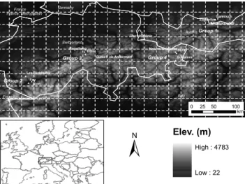
Fig. 1.Location of the twelve meteorological stations (triangles), and ERA-Interim 0.25◦×0.25◦grids (dashed line). Twelve stations were clustered into four groups according to the different ERA-Interim grids. The elevation ranges from 22 m to 4783 m a.s.l., with a DEM resolution of 90 m.

The geopotential height was calculated by the normalization of the geopotential over the gravity.

2.2 Test sites

The data from twelve test sites, all located in the German and Swiss Alps, have been used in the analysis. The stations are located within four different ERA-Interim grid elements and can be treated as four clusters of three stations (one at the valley bottom, one at the crest region and a station in between). A detailed description of the measurements and of the location of the different stations is given in Fig. 1 and Table 1. All measurements were aggregated to 3-hourly (T3h)

and daily (Td)data for a later comparison with ERA-Interim

data (Table 1). Days with missing values were excluded and were not used for any further analysis.

One important but difficult to answer question is whether individual stations might be used by ERA-Interim for as-similation purposes. If assimilated, the ERA-interim pre-dictions are not fully independent from the observed data which were subsequently used for calibration and validation of the suggested downscaling methods. However, even a di-rect contact with the ECMWF personnel could not give a clear answer to this question (Pappenberger, personal com-munication, 2012). It is probable that the data of the sta-tions Zugspitze, Garmisch and Sion are used for assimila-tion, given their status as WMO SYNOP stations (Simmons et al., 2010; Dee et al., 2011). According to the information of the ECMWF it can be assumed that at least the major-ity of the stations at Zugspitzplatt, Fey, Les Diablerets, En-gelberg, G¨utsch ob Andermatt, Titlis, Scuol, Buffalora and Naluns/Schlivera are not used by ERA-Interim and therefore represent fully independent data set.

E E E E E E E E E E E E E E E E E E E E E E E

# # # # # # ## # ### ! ! ! ! ! ! ! ! ! ! ! ! ! ! ! ! ! ! ! ! ! ! ! ! ! ! ! ! ! ! ! ! ! ! ! ! ! ! ! ! ! ! ! ! ! ! ! ! ! ! ! ! ! ! ! ! ! ! ! ! ! ! ! ! ! ! ! ! ! ! ! ! ! ! ! ! ! ! ! ! ! ! ! ! ! ! ! ! ! ! ! ! ! ! ! ! ! ! ! ! ! ! ! ! ! ! ! ! ! ! ! ! ! ! ! ! ! ! ! ! ! ! ! ! ! ! ! ! ! ! ! ! ! ! ! ! ! ! ! ! ! ! ! ! ! ! ! ! ! ! ! ! ! ! ! ! ! ! ! ! ! ! ! ! ! ! ! ! ! ! ! ! ! ! ! ! ! ! ! ! ! ! ! ! ! ! ! ! ! ! ! ! ! ! ! ! ! ! ! ! ! ! ! ! ! ! ! ! ! ! ! ! ! ! ! ! ! ! ! ! ! ! ! ! ! ! ! ! ! ! ! ! ! ! ! ! ! ! ! ! ! ! ! ! ! ! ! ! ! ! ! ! ! ! ! ! ! ! ! ! ! ! ! ! ! ! ! ! ! ! ! ! ! ! ! ! ! ! ! ! ! ! ! ! ! !

0.9 0.9 1.8 0.8 1.7 1.3 1.1 1.7 1.1 0.9 0.9 0.9 1.2 1.1 1.2 1.2 1.6 1.6

1.2 1.1 1.2 1.5 1.4 0.9 0.8 1.1 1.9 2.1 2.6 2.8 2.8 1.7 1.2 1.5 1.8 1.2 1.8 1.8

1.1 0.9 0.8 0.7 0.8 0.8 1.3 1.8 2.5 2.1 1.9 1.5 3.3 1.8 1.1 1.2 1.5 1.3

0.9 1.5 1.8 0.8 1.5 1.8 1.7 1.5 2.6 1.5 1.1 1.3 1.4 1.4 2.3 1.1 1.3 2.1 1.2

1.6 0.9 1.9 2.3 2.2 2.4 0.9 0.8 1.2 2.6 1.4 1.6 1.8 2.7 1.8 2.4 4.8 2.7 1.2

0.8 2.3 1.7 0.9 0.9 1.1 2.9 4.2 3.1 2.8 2.3 1.5 2.8 2.6 2.2 1.2 1.2 2.9 2.5

3.3 2.3 2.1 2.3 3.6 3.7 1.3 1.2 2.1 3.9 2.9 2.4 4.4 1.1 4.3 2.8

2.1 1.3 1.5 1.2 2.1 4.1 5.5 1.7 1.3 1.5 3.9 1.3 2.1 1.2 1.5 1.8 3.9 0.9 3.6

1.8 3.4 3.8 4.8 4.7 1.1 4.3 3.2 3.5 1.4 0.9 1.3 2.5 0.9 1.1

3.1 1.1 3.1 1.2 1.1 3.7 3.4 3.6 3.9 3.7 2.8 3.4 2.3 2.7 1.1 0.8 2.2

3 1 1

1

2 1 1

1 2

1 1

1 2

1 2 4 2 5

2 1

1 4 3 4 1 1

3 3 3 4

Correlation (r)

0.94 - 0.95 0.95 - 0.96 0.96 - 0.97 0.97 - 0.98 0.98 - 0.99

0 25 50 100

km

±

Fig. 2. Correlation and MAE (◦C) between daily mean ERA-Interim 2 m temperature and E-2 OBS data (0.25◦_×_0.25◦_,

pe-riod from 1979 to 2010) extended Simmons’ investigation (5◦×5◦, monthly, period from 1989 to 2001). The values labeled in the grid are the MAEs. The dots are the center points of ERA-Interim grid, the crosses are the center points of E-OBS grid and the triangles are the test sites. ERA-Interim and E-OBS grids are shifted in latitude and longitude direction by 0.125◦_{, i.e. the center point of the E-OBS}

grid is located at the cross junction of four ERA-Interim grids. The average value of every four ERA-Interim points was calculated for the corresponding E-OBS grid.

2.3 E-OBS database

We used E-OBS data of the EU-FP6 ENSEMBLES project for validating the large scale error of the ERA-Interim re-sults. The European daily high-resolution gridded data set of near-surface temperature (minimum, mean and maximum temperature) and precipitation (E-OBS) was operated as part of the EU-FP6 ENSEMBLES project (Haylock et al., 2008). Daily data were produced using a three-step interpolation on the basis of around 2300 stations while taking the ele-vation dependency of temperature into account (Haylock et al., 2008). The E-OBS dataset was produced for represent-ing the best estimates of grid box averages. Gridded 0.25◦

and 0.5◦

latitude/longitude data were available as well as a 0.22◦

and 0.44◦

rotated pole grid with the North Pole at 39.25◦

N, 162◦

W. The available data covers a large area (25◦

–75◦

N, 40◦

W–75◦

E) and a long time period. Here, we used the daily mean temperature with a 0.25◦_×

0.25◦

spa-tial resolution from E-OBS version 6.0, which was released in April 2012 and which covers the period from 1950–2011. The time period of 1979–2010 was extracted for a compar-ison with the 0.25◦_×_0.25◦ _{ERA-Interim 2 m temperature}

data. ERA-Interim and E-OBS data are shifted in latitude and longitude direction by 0.125◦

(4)

Table 1.Test sites information (ERA height is the ERA-Interim model elevation).

Altitude ERA height

Site latitude longitude (m a.s.l) (m a.s.l) Time Series

Group 1 Garmisch 47.48 11.07 719 1287 1979–2010 Zugspitzplatt 47.41 11.00 2250 1999–2010 Zugspitze 47.42 10.99 2964 1979–2010

Group 2

Sion 46.22 7.33 482

1408 2002–2004

Fey 46.19 7.27 737

Les Diablerets 46.33 7.20 2966

Group 3

Engelberg 46.82 8.41 1036

1432 1994–2010 G¨utsch ob Andermatt 46.65 8.62 2287

Titlis 46.77 8.43 3040

Group 4

Scuol 46.79 10.28 1304

1818 1999–2010 Buffalora 46.65 10.27 1968

Naluns/Schlivera 46.82 10.26 2400

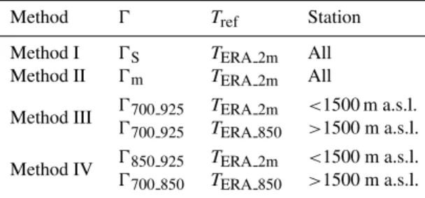
2.4 Elevation correction methods

Lapse rates (Ŵ) describe the decrease ofTa with elevation.

Equation (1) was used for all of the four presented correc-tion methods, but the calculacorrec-tion ofTrefandŴ varied.Tref

is the reference temperature, which was either defined by the ERA-Interim 2 m temperature (TERA 2m)or the ERA-Interim

temperature at the 850 hPa pressure level (TERA 850).

Tt=Tref+Ŵ×1h (1)

We used four different methods for calculatingŴ, Method (I) specific monthly lapse rates (ŴS) extracted from

lit-erature, Method (II) measured lapse rates (ŴM), which

were calculated on the basis of two meteorological sta-tions covering the maximum elevation range of the area, and Method (III) and (IV) ERA-Interim lapse rates (Ŵ700 925

and Ŵ850 925/Ŵ700 850) which were calculated on the basis

of temperatures at different pressure levels. Method I made use of monthly values of ŴS, which were calculated from

the monthly mean maximum and minimum temperature data published by Kunkel (1989) and Liston and Elder (2006) (Ta-ble 2). These values have been widely applied in Earth sur-face modeling and their temporal resolution of one month can be seen as a standard with respect to generalized lapse rates (Bernhardt and Schulz, 2010; Mernild et al., 2009; Liston et al., 2008).

Method II used measured data from two meteorological stations for calculating 3-hourly and daily lapse rates. We used the highest and lowest elevated station per group for this calculation (Table 1). The lower elevated station repre-sents the conditions at the valley bottom, while the higher el-evated station is representative for the crest region. Method II was used as a benchmark for comparison with all other meth-ods. Since stations at high elevation that are able to properly represent the meteorology are rare, other correction meth-ods that are independent of surface measurements have to

Fig. 3. Schematic illustration of measured lapse rate and ERA-Interim derived lapse rates for Group 1.Ŵmwas calculated based

on the two largest-elevation-difference stations (e.g. Garmisch and Zugspizte station). Temperatures as well as the geopotential heights of the 700 hPa, 850 hPa and 925 hPa level were used for calculating

Ŵ_{700 925},Ŵ_{850 925}andŴ_{700 850}. The dashed blue line represents

the mean geopotential height of the corresponding pressure level (for the period 1979–2010).

be developed (Blandford et al., 2008; Pages and Miro, 2010; Rolland, 2003).

In the following, we introduce two methods, which are based on ERA-Interim internal temperature gradients for ad-dressing this need. Temperatures as well as the geopotential heights of the 700 hPa, 850 hPa and 925 hPa level were used for calculatingŴ700 925,Ŵ850 925andŴ700 850. This was done

by calculating temperature differences between the 700 hPa and 850 hPa (Ŵ700 850), 700 hPa and 925 hPa (Ŵ700 925), as

well as 850 hPa and 925 hPa (Ŵ850 925) level (Fig. 3) and

(5)

Table 2.Fixed monthly lapse rates extracted from Kunkel (1989) and Liston and Elder (2006).

Jan Feb Mar Apr May Jun Jul Aug Sep Oct Nov Dec

Lapse rate (◦C km−1) −4.4 −5.9 −7.1 −7.8 −8.1 −8.2 −8.1 −8.1 −7.7 −6.8 −5.5 −4.7

Table 3.Applied lapse rate (Ŵ) and reference temperature (T_ref)of four correction methods for twelve test stations.

Method Ŵ T_ref Station

Method I Ŵ_S T_{ERA 2m} All Method II Ŵm TERA 2m All

Method III Ŵ700 925 TERA 2m <1500 m a.s.l.

Ŵ_{700 925} T_{ERA 850} >1500 m a.s.l.

Method IV Ŵ850 925 TERA 2m <1500 m a.s.l.

Ŵ_{700 850} T_{ERA 850} >1500 m a.s.l.

A differentiation intoŴ850 925andŴ700 850was introduced

to accommodate different atmospheric conditions and there-fore dominant controls on surface temperature. While low al-titudes are often influenced by local circulation patterns (rep-resented byŴ850 925), temperature conditions at higher

ele-vations (represented byŴ700 850)are more representative of

free air flow conditions (Mahrt et al., 2001; Pepin and Seidel, 2005). Tabony (1985) noted that the transition from local cir-culation dominated to free air-dominated temperatures could be found at approximately 1400 m a.s.l. within the Austrian Alps. This estimate is used for splitting the temperature gra-dient into a lower, local flow dominated and a higher, free air flow dominated, gradient. For our test sites, the 850 hPa level, varying around 1500 m a.s.l., was used as a transition level dividing the local circulation dominated zone, from the free air flow dominated zone. We usedTERA 850 instead of

TERA 2mas a basis for the calculation of the elevation

correc-tion for locacorrec-tions higher than 1500 m. Figure 3 illustrates (for stations in group 1 as an example) the different parameters used in Eq. (1). Method III usesTERA 2m andŴ700 925 for

the calculation of the temperature (Ta)at Garmisch station

andTERA 850 and Ŵ700 925 for Zugspitze and Zugspitzplatt

stations. In Method IV,TERA 2m andŴ850 925 are the basis

for the calculation ofTa at Garmisch station andTERA 850

as well asŴ700 850 for Zugspitze and Zugspitzplatt stations

(Table 3).

3 Results

3.1 Validation of the uncorrected ERA-Interim

temperature data

In a first step, the quality of the uncorrected ERA-Interim data was analysed. We used a comparison of ERA and CRUTEM3 (gridded observations) data of Simmons et

al. (2010), E-OBS data and station measurements for this comparison. Simmons et al. (2010) have shown that the large scale error of ERA-Interim 2 m temperature is gen-erally small in Europe. They compared 40 and ERA-Interim monthly temperatures against CRUTEM3 results by using a 5◦_×

5◦

grid. They found a high temporal correla-tion (r=₀.997) between CRUTEM3 and ERA-Interim re-sults for the period from 1989 to 2001, with respect to Eu-rope. It was shown that the accordance of ERA-Interim and CRUTEM3 is generally good with respect to large-scale pat-terns and magnitudes (Simmons et al., 2010). The investi-gations of Simmons et al. (2010) are extended here by us-ing E-OBS data, given higher temporal (1 day) and spatial resolution (0.25◦_{) and the availability of the data for the}

pe-riod from 1979–2010. A very good agreement between ERA-Interim and E-OBS data with high correlation values (0.947– 0.992) was found (Fig. 2). Compared to Simmons’ work, our comparison adopted a higher temporal resolution and a longer time period. The mean average error (MAE) between the two datasets became larger in the Alpine parts of the test area and could be connected to elevation differences be-tween ERA-Interim model elevations and E-OBS grid eleva-tions. By taking elevation differences into account and using Method I for data interpolation errors could be reduced and led to a reduction of the average MAE from 1.98 to 1.29◦

C, and an increase of the correlation coefficient from 0.963 to 0.992. The simple elevation correction demonstrated that the existing errors can be well connected to elevation effects and that the large scale error of ERA-Interim is small in general. A comparison of ERA-Interim results with the available meteorological stations underlined these results (Fig. 4). It can be seen that the 0.25◦

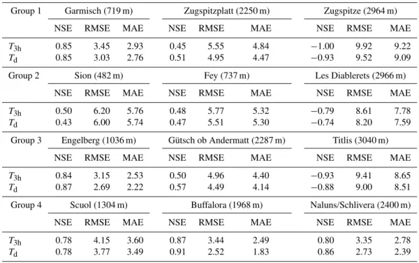
ERA-Interim results show large deviations with respect to point measurements. This is es-pecially true in case the elevation of the stations differ sig-nificantly from mean elevation of the corresponding ERA-Interim grid elements. We found the largest biases for the higher elevated stations, while the stations located at the valley bottom show the highest accordance to the model (Table 4).

3.2 Temporal variability of the lapse rates

The different lapse rates (ŴS, ŴM, Ŵ700 925 and

Ŵ850 925/Ŵ700 850, see Sect. 2.4) show a different

(6)

Table 4.Comparison of ERA-Interim 2 m temperature with 3-hourly and daily data of twelve meteorological stations. The NSE as well as the RMSE and MAE in◦C are also listed, and the elevations (m) are labeled in brackets.

Group 1 Garmisch (719 m) Zugspitzplatt (2250 m) Zugspitze (2964 m)

NSE RMSE MAE NSE RMSE MAE NSE RMSE MAE

T_3h 0.85 3.45 2.93 0.45 5.55 4.84 −1.00 9.92 9.22 T_d 0.85 3.03 2.76 0.51 4.95 4.47 −0.93 9.52 9.09

Group 2 Sion (482 m) Fey (737 m) Les Diablerets (2966 m)

T_3h 0.50 6.20 5.76 0.48 5.77 5.32 −0.79 8.61 7.78 T_d 0.43 6.00 5.74 0.47 5.51 5.30 −0.74 8.20 7.59

Group 3 Engelberg (1036 m) G¨utsch ob Andermatt (2287 m) Titlis (3040 m)

T_3h 0.84 3.15 2.53 0.50 4.96 4.40 −0.93 9.41 8.65 T_d 0.87 2.69 2.22 0.57 4.49 4.14 −0.88 9.00 8.51

Group 4 Scuol (1304 m) Buffalora (1968 m) Naluns/Schlivera (2400 m)

T_3h 0.78 4.15 3.60 0.87 3.44 2.49 0.80 3.35 2.78 T_d 0.78 3.77 3.49 0.91 2.52 1.83 0.86 2.73 2.39

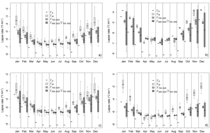
value per month. It can be seen that the lapse rates are generally smaller in winter but showed a higher variability during these colder months (October–February). Warmer months were characterized by lapse rates in the range of −6◦_{C km}−1 _to ₋₇◦_{C km}−1 _{and by a low inter-monthly}

variability (April–August). March and September represent transition months, where the regime changed from winter to summer or from summer to winter conditions. The between-group variability of the derived lapse rates also varied significantly. Group 2 shows the lowest variability, due to the very short time period of data availability. ŴS

generally represents the largest temperature gradient and is significantly different from the measurements, especially during the summer months.Ŵ700 925 and Ŵ850 925/Ŵ700 850

show larger variations during winter time and dynamics which are closer to the measurements (ŴM). Only the

temporal dynamics of Group 4 are not well covered by the ERA-Interim lapse rates. This group is located in the central Alps where the respective ERA-Interim grid elements do also show a large deviation from the E-OBS data. The overall difference between measured and modeled lapse rates is in general small in summertime (June–August) and shows stronger deviations in winter time (November–February), possibly due to frequent local inversion events during winter months that cannot be reproduced by the ERA-Interim model.

3.3 Evaluation of correction methods

In order to evaluate the presented correction methods, three statistical accuracy measures were used. The root mean square error (RMSE) and mean absolute error (MAE) are used for an assessment of the bias between corrected tem-perature and observation (Eqs. 2 and 3). The Nash-Sutcliffe efficiency coefficient (NSE) evaluates the performance of the correction methods using Eq. (4), which ranges from 1 (per-fect fit) to minus infinity. A negative value of the NSE indi-cates that the model is a worse estimator than the mean of the observed data (Nash and Sutcliffe, 1970).

RMSE= v u u t1

N

N X

t=1

Tot−Tct

2

(2)

MAE= 1

N

N X

t=1

T_ot−T_ct

(3)

NSE=₁− N P

t=1

Tot−Tct

2

N P

t=1

Tot−To

2

(4)

withT_ot= observed temperature at timet,T_ct= corrected tem-perature at timet, andN= number of records.

The overall performance of the 4 correction methods is summarized in Table 5. Method III and IV outperformed Method II moderately regardless of whetherT3h orTddata

(7)

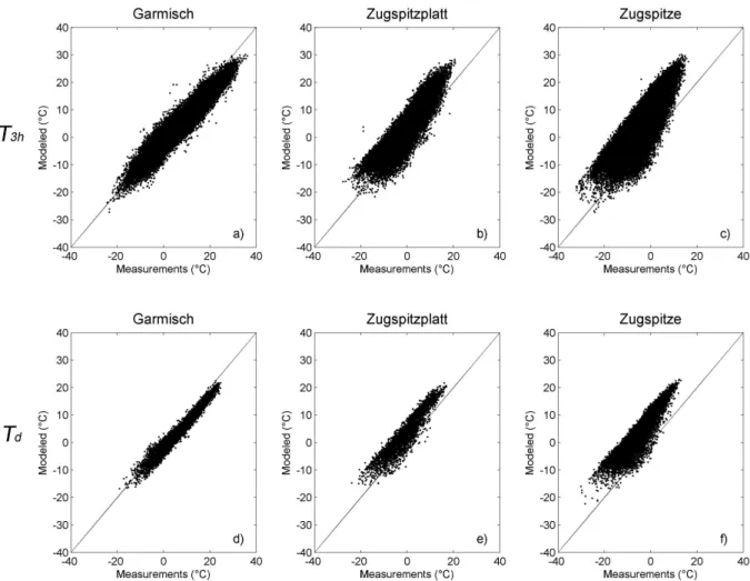
Fig. 4.The scatter plots show the comparison of 3-hourly ERA-Interim 2 m temperature and meteorological stations for Group 1, (a) Garmisch station (1979–2010),(b)Zugspitzplatt station (1999–2010) and(c)Zugspitze station (1979-2010). All the related accuracy mea-sures can be found in Table 4.

Table 5.Comparison of measurements with corrected 3-hourly and daily data for 4 methods by averaging NSE, RMSE and MAE statis-tics of all 12 test sites.

T_3h T_d Method NSE RMSE MAE NSE RMSE MAE

I 0.78 3.37 2.60 0.85 2.59 2.09 II 0.91 2.31 1.77 0.95 1.63 1.25 III 0.92 2.21 1.64 0.95 1.57 1.15 IV 0.92 2.21 1.65 0.95 1.56 1.14

The specific performance of the four correction methods with respect to 3-hourly temperature data is summarized in Table 6. Figure 6 gives a more detailed visualization of the results given by Group 1. Method I worked well for stations located in the valley bottom, showed only moderate improve-ments for the average altitude stations, and even failed for the higher elevated stations (Table 6 and Fig. 6). Station Fey is an exception, showing the second best results (with respect

to the NSE, RMSE and MAE) when Method I is applied (Ta-ble 6). Method II delivered the best results for the valley sta-tions, but showed also acceptable results for the average alti-tude and high altialti-tude stations. However, Method III and IV outperformed Method II for seven out of eight average and high altitude stations (Table 6). The reduction of the MAE for the valley stations was between 34.0 % (Engelberg) and 73.6 % (Sion), when using Method II. The MAE could also be improved for the average altitude stations (improvement between 53.8 % and 59.7 %) with the exception of Buffalora, which were less accurate than the original ERA-Interim re-sults (2.49◦

C, method I; 2.67◦

C, Method II). The MAE at the high altitude stations was reduced to between 1.2◦

C (Naluns/Schlivera) and 7.8◦

(8)

Fig. 5.Boxplots of monthly lapse rates for(a)Group 1 (1979–2010),(b)Group 2 (2002–2004),(c)Group 3 (1994-2010) and(d)Group 4 (1999–2010).Ŵ_S(short horizontal line),Ŵ_M(light gray),Ŵ_{700 925}(medium gray) andŴ_{850 925}/Ŵ_{700 850}(dark gray). Thick horizontal lines in boxes show the median values. Boxes indicate the inner-quantile range (25 % to 75 %) and the whiskers show the full range of the values.

to 28 February 1996. The measurements show frequent and rapid changes with respect to the temperature. The tempera-tures reached high values, around 30◦_{C, and afterwards fall}

back to normal values (below of 0◦

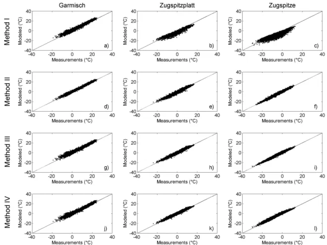
C) while the surroundings stations show no anomalies. Therefore, a measurement error at station Titlis has to be expected. Method II which is based on the measurements is consequently forcing the model re-sults into the direction of the nonconforming measurements. The other methods which are independent of the station mea-surements do not reproduce this error. This is another exam-ple why methods which are independent of surface data are useful in high alpine areas where error-prone measurements are common. Furthermore, Methods III and IV performed very well at high altitude stations. The MAE at the average altitude stations could be reduced by 57.9 % to 74.7 % and by 59.4 % to 87.9 % for the high altitude stations. Nevertheless, the differences between Methods III and IV are negligible and an application of the simpler Method III seems to be suf-ficient, at least for the stations used in this study.

Figure 7 illustrates the performance of all 4 methods with respect to daily average temperatures, again by taking Group 1 as an example. While the accuracy of the correction re-sults was similar when compared to the use of 3-hourly data, some additional interesting aspects can be analyzed for the aggregated data. For example, daily averages as well as daily

minima and maxima temperature data are often used for char-acterizing local sites given current or predicted future climate conditions. Figure 7 clearly shows that the results at the lower end of the temperature spectrum were overestimated while warmer temperatures were underestimated. The extrapola-tion of the original ERA-Interim data or of data downscaled using Method I would therefore lead to a systematic misin-terpretation of minimum and maximum values. This effect could only be eliminated when site specific lapse rates were used. This again is a strong argument against a general ap-plication of lapse rates, which are only oriented on station-ary temperature gradient, but which do not factor in the local characteristics of a specific site.

4 Discussion and conclusion

(9)

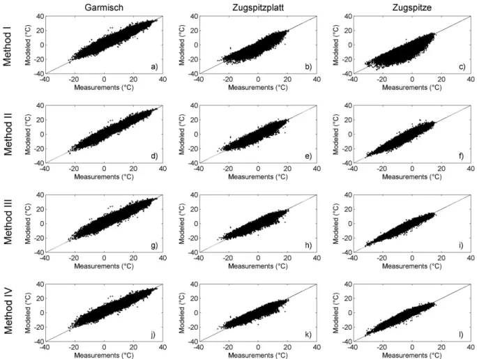
Fig. 6.The scatter plots show a comparison of measured and modeled 3-hourly temperatures for Group 1.(a, d, g, j)show the results of the different methods for Garmisch (1979–2010),(b, e, h, k)for Zugspitzplatt (1999–2010) and(c, f, I, l)for Zugspitze (1979–2010). All of the related accuracy measures can be found in Table 6.

latitude/longitude grids, and others, can affect the observed difference between the model and the measurements (Dee, 2005; Dee et al., 2011).

We were able to demonstrate that the large scale biases of ERA-Interim for temperature are very small, except for re-gions were the elevation differences between model grid and real world are high, as for example in the central Alps. Also, the total integral error between modeled and measured data was strongly reduced by using lapse rate approaches for ele-vation correction. In that context ERA-Interim internal lapse rate showed a better performance than observed lapse rate and reduced the RMSE and MAE for high altitudes. How-ever, it has to be noted that even for some periods and loca-tions significant differences between modeled and observed lapse rates could be observed.

The comparison between ERA-Interim 2 m temperature and E-OBS gridded data for the period from 1979 to 2010 indicates that elevation is the driving force for the observed error which therefore should be able to be corrected via el-evation based approaches, such as lapse rates. Subsequently,

0.25◦_×

0.25◦

3-hourly and daily ERA-Interim 2 m tempera-ture data were compared with local measurements at twelve stations within the German and Swiss Alps. The comparison has illustrated that there is a need for a correction of ERA-Interim data if it should be used at a given point in the moun-tains. The results in Table 4 make clear that a correction is neccessary for accounting for elevation driven temperature variations in heterogeneous mountain terrain, which cannot be represented by the original ERA-Interim grid.

Four different methods were used to derive the needed lapse rates Ŵ: a fixed monthly lapse rate (ŴS) extracted

from the literature (Method I); a measured lapse rate (ŴM)

(Method II); and ERA-Interim model internal lapse rates

(Ŵ700 925 andŴ850 925/Ŵ700 850)derived from predictions at

different pressure levels (Method III and IV).

Observed changes of lapse rates with elevation and with time demonstrated that the use of fixed lapse rates (ŴS)were

(10)

Table 6.Comparison of measurements with corrected 3-hourly and daily data for group 1–4. The NSE as well as the RMSE and MAE in◦_C

are also listed.

Group 1 Garmisch Zugspitzplatt Zugspitze

Method NSE RMSE MAE NSE RMSE MAE NSE RMSE MAE

T_3h I 0.91 2.70 2.13 0.71 4.07 3.11 0.59 4.47 3.46 II 0.96 1.84 1.40 0.88 2.56 1.95 0.93 1.84 1.40 III 0.92 2.44 1.87 0.91 2.31 1.74 0.96 1.45 1.12 IV 0.91 2.62 1.99 0.91 2.29 1.73 0.94 1.73 1.33

T_d I 0.94 2.00 1.64 0.79 3.22 2.61 0.74 3.47 2.89 II 0.98 1.07 0.82 0.94 1.76 1.37 0.98 1.07 0.82 III 0.95 1.69 1.29 0.96 1.36 1.07 0.98 1.00 0.78 IV 0.94 1.91 1.43 0.97 1.31 1.03 0.96 1.32 1.00

Group 2 Sion Fey Les Diablerets

T_3h I 0.92 2.47 1.98 0.90 2.60 2.00 0.46 4.74 3.68 II 0.94 2.03 1.52 0.83 3.21 2.46 0.90 2.03 1.52 III 0.92 2.45 1.89 0.87 2.88 2.24 0.89 2.13 1.31 IV 0.93 2.32 1.81 0.90 2.55 1.99 0.90 2.04 1.25

T_d I 0.94 1.92 1.54 0.93 1.94 1.47 0.60 3.91 3.26 II 0.96 1.56 1.15 0.89 2.46 1.90 0.94 1.56 1.15 III 0.94 1.90 1.46 0.92 2.18 1.64 0.92 1.79 1.02 IV 0.95 1.74 1.35 0.94 1.83 1.40 0.93 1.62 0.86

Group 3 Engelberg G¨utsch ob Andermatt Titlis

T_3h I 0.89 2.60 2.01 0.78 3.33 2.52 0.56 4.50 3.44 II 0.92 2.19 1.67 0.89 2.35 1.78 0.89 2.19 1.67 III 0.90 2.51 1.89 0.95 1.54 1.18 0.92 1.92 1.18 IV 0.90 2.48 1.86 0.95 1.50 1.16 0.92 1.94 1.24

T_d I 0.93 2.02 1.61 0.86 2.57 2.05 0.70 3.57 2.89 II 0.96 1.53 1.18 0.95 1.59 1.19 0.95 1.53 1.18 III 0.94 1.82 1.38 0.98 1.01 0.77 0.95 1.48 0.88 IV 0.94 1.85 1.41 0.98 0.96 0.74 0.95 1.51 0.97

Group 4 Scuol Buffalora Naluns/Schlivera

T_3h I 0.94 2.26 1.80 0.89 3.21 2.46 0.79 3.45 2.66 II 0.95 2.00 1.57 0.86 3.51 2.67 0.93 2.00 1.57 III 0.94 2.23 1.75 0.89 3.22 2.46 0.96 1.47 1.10 IV 0.93 2.38 1.87 0.89 3.16 2.42 0.96 1.51 1.13

T_d I 0.97 1.43 1.14 0.93 2.21 1.59 0.85 2.85 2.34 II 0.97 1.51 1.23 0.92 2.43 1.72 0.96 1.51 1.23 III 0.97 1.49 1.18 0.93 2.18 1.57 0.98 0.99 0.78 IV 0.96 1.58 1.23 0.94 2.14 1.55 0.98 0.95 0.75

situation where the complete vertical elevation/temperature gradient is covered by two stations providing continuously measured lapse rates. While this approach provided the best results, it would be interesting to analyze how far these mea-sured lapse rates could be extrapolated in a spatial context.

(11)

Fig. 7.The scatter plots show a comparison of measured and modeled daily temperature averages for Group 1.(a, d, g, j)show the results of the different methods for Garmisch (1979–2010),(b, e, h, k)for Zugspitzplatt (1999–2010) and(c, f, I, l)for Zugspitze (1979–2010). All of the related accuracy measures can be found in Table 6.

the direction of implausible temperatures if one of the sta-tions which are used for calculating the lapse rate delivers incorrect measurements.

Method III and IV represent alternatives for deriving tem-perature lapse rates by using (global climate) model (here ERA-Interim) internal lapse rates from representative pres-sure levels. Both methods showed a convincing performance when compared to measured data of the twelve stations, again especially for those in higher elevations. The ERA-Interim internal lapse rate is a useful tool for correcting the original output data to the station scale, even if they un-derestimate the observed lapse rates for most of the entire season. The additional implementation of an internal base-line at approximately 1500 m and the calculation of sepa-rate lapse sepa-rates above and below (Method IV), allowed a vertical differentiation and the consideration of local circula-tion effects (below) and the dominance of free air condicircula-tions (above) on the temperature distribution (Mahrt, 2006; Rol-land, 2003; Blandford et al., 2008). However, results only showed minimal differences between Method III and IV for the used test sites.

So far, our analysis has been limited to German and Swiss Alps with 12 meteorological stations providing cali-bration/validation data sets for testing developed correction methods. It will be necessary to extend this analysis to dif-ferent high mountainous areas around the world. It should also be investigated whether other global reanalysis products, using different land surface representations in their climate models can be used in context with the presented approach. Also, the potential of extending our approach to other me-teorological variables has to be explored and is a topic of on-going and future research.

(12)

two anonymous reviewers for their valuable comments and also appreciate the editor’s suggestion.

Edited by: J. Seibert

References

Barry, R. G.: Mountain Climatology and Past and Potential Fu-ture Climatic Changes in Mountain Regions – a Review, Mt Res. Dev., 12, 71–86, 1992.

Bernhardt, M. and Schulz, K.: SnowSlide: A simple routine for cal-culating gravitational snow transport, Geophys. Res. Lett., 37, L11502, doi:10.1029/2010gl043086, 2010.

Berrisford, P., Dee, D., Fielding, K., Fuentes, M., Kallberg, P., Kobayashi, S., and Uppala, S.: The ERA-Interim archive (version 1.0), ERA Report Series: European Centre for Medium Range Weather Forecasts, 2009.

Berrisford, P., Kallberg, P., Kobayashi, S., Dee, D., Uppala, S., Sim-mons, A. J., Poli, P., and Sato, H.: Atmospheric conservation properties in ERA-Interim, Q. J. Roy. Meteorol. Soc., 137, 1381– 1399, doi:10.1002/Qj.864, 2011.

Blandford, T. R., Humes, K. S., Harshburger, B. J., Moore, B. C., Walden, V. P., and Ye, H. C.: Seasonal and synop-tic variations in near-surface air temperature lapse rates in a mountainous basin, J. Appl. Meteorol. Clim., 47, 249–261, doi:10.1175/2007jamc1565.1, 2008.

Bolstad, P. V., Swift, L., Collins, F., and Regniere, J.: Measured and predicted air temperatures at basin to regional scales in the south-ern Appalachian mountains, Agr. Forest Meteorol., 91, 161–176, 1998.

Cullen, R. M. and Marshall, S. J.: Mesoscale Tempera-ture Patterns in the Rocky Mountains and Foothills Re-gion of Southern Alberta, Atmos. Ocean, 49, 189–205, doi:10.1080/07055900.2011.592130, 2011.

Dee, D. and Uppala, S.: Variational bias correction in ERA-Interim, ECMWF Newsletter, No. 119, 21–29, 2009.

Dee, D. P.: Bias and data assimilation, Q. J. Roy. Meteorol. Soc., 131, 3323–3343, doi:10.1256/Qj.05.137, 2005.

Dee, D. P., Uppala, S. M., Simmons, A. J., Berrisford, P., Poli, P., Kobayashi, S., Andrae, U., Balmaseda, M. A., Balsamo, G., Bauer, P., Bechtold, P., Beljaars, A. C. M., van de Berg, L., Bid-lot, J., Bormann, N., Delsol, C., Dragani, R., Fuentes, M., Geer, A. J., Haimberger, L., Healy, S. B., Hersbach, H., Holm, E. V., Isaksen, L., Kallberg, P., Kohler, M., Matricardi, M., McNally, A. P., Monge-Sanz, B. M., Morcrette, J. J., Park, B. K., Peubey, C., de Rosnay, P., Tavolato, C., Thepaut, J. N., and Vitart, F.: The ERA-Interim reanalysis: configuration and performance of the data assimilation system, Q. J. Roy. Meteorol. Soc., 137, 553– 597, doi:10.1002/Qj.828, 2011.

DeGaetano, A. T. and Belcher, B. N.: Spatial interpolation of daily maximum and minimum air temperature based on meteorologi-cal model analyses and independent observations, J. Appl. Me-teorol. Clim., 46, 1981–1992, doi:10.1175/2007JAMC1536.1, 2007.

Dodson, R. and Marks, D.: Daily air temperature interpolated at high spatial resolution over a large mountainous region, Clim. Res., 8, 1–20, 1997.

Gruber, S.: Derivation and analysis of a high-resolution estimate of global permafrost zonation, The Cryosphere, 6, 221–233,

doi:10.5194/tc-6-221-2012, 2012.

Hamlet, A. F. and Lettenmaier, D. P.: Production of temporally con-sistent gridded precipitation and temperature fields for the conti-nental United States, J. Hydrometeorol., 6, 330–336, 2005. Haylock, M. R., Hofstra, N., Tank, A. M. G. K., Klok, E.

J., Jones, P. D., and New, M.: A European daily high-resolution gridded data set of surface temperature and precipi-tation for 1950–2006, J. Geophys. Res.-Atmos., 113, D20119, doi:10.1029/2008jd010201, 2008.

Ishida, T. and Kawashima, S.: Use of Cokriging to Estimate Sur-face Air-Temperature from Elevation, Theor. Appl. Climatol., 47, 147–157, 1993.

Kunkel, E. K.: Simple Procedures for Extrapolation of Humidity Variables in the Mountainous Western United States, J. Climate, 2, 656–669, 1989.

Laughlin, G. P.: Minimum Temperature and Lapse-Rate in Com-plex Terrain – Influencing Factors and Prediction, Arch. Meteor. Geophy. B, 30, 141–152, 1982.

Liston, G. E. and Elder, K.: A meteorological distribution system for high-resolution terrestrial modeling (MicroMet), J. Hydrom-eteorol., 7, 217–234, 2006.

Liston, G. E., Hiemstra, C. A., Elder, K., and Cline, D. W.: Mesocell Study Area Snow Distributions for the Cold Land Processes Experiment (CLPX), J. Hydrometeorol., 9, 957–976, doi:10.1175/2008jhm869.1, 2008.

Lundquist, J. D. and Cayan, D. R.: Surface temperature patterns in complex terrain: Daily variations and long-term change in the central Sierra Nevada, California, J. Geophys. Res.-Atmos., 112, D11124, doi:10.1029/2006jd007561, 2007.

Mahrt, L., Vickers, D., Nakamura, R., Soler, M. R., Sun, J. L., Burns, S., and Lenschow, D. H.: Shallow drainage flows, Bound.-Lay. Meteorol., 101, 243–260, 2001.

Mahrt, L.: Variation of surface air temperature in complex terrain, J. Appl. Meteorol. Clim., 45, 1481–1493, 2006.

Maraun, D., Wetterhall, F., Ireson, A. M., Chandler, R. E., Kendon, E. J., Widmann, M., Brienen, S., Rust, H. W., Sauter, T., Themessl, M., Venema, V. K. C., Chun, K. P., Goodess, C. M., Jones, R. G., Onof, C., Vrac, M., and Thiele-Eich, I.: Precipita-tion Downscaling under Climate Change: Recent Developments to Bridge the Gap between Dynamical Models and the End User, Rev. Geophys., 48, Rg3003, doi:10.1029/2009rg000314, 2010. Marshall, S. J., Sharp, M. J., Burgess, D. O., and Anslow, F. S.:

Near-surface-temperature lapse rates on the Prince of Wales Icefield, Ellesmere Island, Canada: implications for regional downscaling of temperature, Int. J. Climatol., 27, 385–398, doi:10.1002/Joc.1396, 2007.

Maurer, E. P., Wood, A. W., Adam, J. C., Lettenmaier, D. P., and Nijssen, B.: A long-term hydrologically based dataset of land surface fluxes and states for the conterminous United States, J. Climate, 15, 3237–3251, 2002.

Mernild, S. H., Liston, G. E., Hiemstra, C. A., Steffen, K., Hanna, E., and Christensen, J. H.: Greenland Ice Sheet sur-face mass-balance modelling and freshwater flux for 2007, and in a 1995–2007 perspective, Hydrol. Process., 23, 2470–2484, doi:10.1002/Hyp.7354, 2009.

(13)

Mokhov, I. I. and Akperov, M. G.: Tropospheric lapse rate and its relation to surface temperature from reanalysis data, Izv Atmos. Ocean Phy.+, 42, 430–438, doi:10.1134/S0001433806040037, 2006.

Mooney, P. A., Mulligan, F. J., and Fealy, R.: Comparison of ERA-40, ERA-Interim and NCEP/NCAR reanalysis data with observed surface air temperatures over Ireland, Int. J. Climatol., 31, 545–557, doi:10.1002/Joc.2098, 2011.

Nash, J. E. and Sutcliffe, J. V.: River flow forecasting through con-ceptual models part I – A discussion of principles, J. Hydrol., 10, 282–290, 1970.

Nieto, H., Sandholt, I., Aguado, I., Chuvieco, E., and Stisen, S.: Air temperature estimation with MSG-SEVIRI data: Calibration and validation of the TVX algorithm for the Iberian Peninsula, Remote Sens. Environ., 115, 107–116, doi:10.1016/j.rse.2010.08.010, 2011.

Pages, M. and Miro, J. R.: Determining temperature lapse rates over mountain slopes using vertically weighted regression: a case study from the Pyrenees, Meteorol. Appl., 17, 53–63, doi:10.1002/Met.160, 2010.

Pepin, N. C. and Seidel, D. J.: A global comparison of surface and free-air temperatures at high elevations, J. Geophys. Res.-Atmos., 110, D03104, doi:10.1029/2004JD005047, 2005. Prihodko, L. and Goward, S. N.: Estimation of air temperature from

remotely sensed surface observations, Remote Sens. Environ., 60, 335–346, 1997.

Prince, S. D., Goetz, S. J., Dubayah, R. O., Czajkowski, K. P., and Thawley, M.: Inference of surface and air temperature, atmo-spheric precipitable water and vapor pressure deficit using Ad-vanced Very High-Resolution Radiometer satellite observations: comparison with field observations, J. Hydrol., 213, 230–249, 1998.

Regniere, J.: Generalized approach to landscape-wide seasonal forecasting with temperature-driven simulation models, Environ. Entomol., 25, 869–881, 1996.

Rolland, C.: Spatial and seasonal variations of air temperature lapse rates in Alpine regions, J. Climate, 16, 1032–1046, 2003. Simmons, A., Uppala, S., Dee, D., and Kobayashi, S.: ERA-Interim:

New ECMWF reanalysis products from 1989 onwards, ECMWF Newsletter, No. 110, 25–35, 2006.

Simmons, A. J., Willett, K. M., Jones, P. D., Thorne, P. W., and Dee, D. P.: Low-frequency variations in surface atmospheric hu-midity, temperature, and precipitation: Inferences from reanal-yses and monthly gridded observational data sets, J. Geophys. Res.-Atmos., 115, D01110, doi:10.1029/2009jd012442, 2010. Stahl, K., Moore, R. D., Floyer, J. A., Asplin, M. G., and McKendry,

I. G.: Comparison of approaches for spatial interpolation of daily air temperature in a large region with complex topography and highly variable station density, Agr. Forest Meteorol., 139, 224– 236, 2006.

Tabony, R. C.: The Variation of Surface-Temperature with Altitude, Meteorol. Mag., 114, 37–48, 1985.

Uppala, S., Dee, D., Kobayashi, S., Berrisford, P., and Simmons, A.: Towards a climate data assimilation system: status updata of ERA-Interim, ECMWF Newsletter, No. 115, 12–18, 2008. Vicente-Serrano, S. M., Saz-Sanchez, M. A., and Cuadrat, J. M.:

Comparative analysis of interpolation methods in the middle Ebro Valley (Spain): application to annual precipitation and tem-perature, Climate Res., 24, 161–180, 2003.