Aerodynamic gradient measurements of the NH3-HNO3-NH4NO3 triad using a wet chemical instrument: an analysis of precision requirements and flux errors

(1)

AMTD

2, 2423–2482, 2009

An analysis of precision requirements and

flux errors

V. Wolffet al.

Title Page

Abstract Introduction

Conclusions References

Tables Figures

◭ ◮

Back Close

Full Screen / Esc

Printer-friendly Version

Interactive Discussion

Atmos. Meas. Tech. Discuss., 2, 2423–2482, 2009 www.atmos-meas-tech-discuss.net/2/2423/2009/ © Author(s) 2009. This work is distributed under the Creative Commons Attribution 3.0 License.

Atmospheric Measurement Techniques Discussions

Atmospheric Measurement Techniques Discussionsis the access reviewed discussion forum ofAtmospheric Measurement Techniques

Aerodynamic gradient measurements of

the NH

₃

-HNO

₃

-NH

₄

NO

₃

triad using a wet

chemical instrument: an analysis of

precision requirements and flux errors

V. Wolff1, I. Trebs1, C. Ammann2, and F. X. Meixner1,3

1

Max Planck Institute for Chemistry, Biogeochemistry and Air Chemistry Department, P.O. Box 3060, 55020 Mainz, Germany

2

Agroscope ART, Air Pollution and Climate Group, 8046 Z ¨urich, Switzerland

3

Department of Physics, University of Zimbabwe, P.O. Box MP 167, Harare, Zimbabwe Received: 15 July 2009 – Accepted: 21 September 2009 – Published: 8 October 2009 Correspondence to: V. Wolff(veronika.wolff@mpic.de)

(2)

AMTD

2, 2423–2482, 2009

flux errors

V. Wolffet al.

Title Page

Tables Figures

◭ ◮

Back Close

Full Screen / Esc

Interactive Discussion Abstract

The aerodynamic gradient method is widely used for flux measurements of ammo-nia, nitric acid, particulate ammonium nitrate (the NH3-HNO3-NH4NO3triad) and other water-soluble reactive trace compounds. The surface exchange flux is derived from a measured concentration difference and micrometeorological quantities (turbulent

ex-5

change coefficient). The significance of the measured concentration difference is cru-cial for the significant determination of surface exchange fluxes. Additionally, mea-surements of surface exchange fluxes of ammonia, nitric acid and ammonium nitrate are often strongly affected by phase changes between gaseous and particulate com-pounds of the triad, which make measurements of the four individual species (NH₃,

10

HNO₃, NH+₄, NO−₃) necessary for a correct interpretation of the measured concentra-tion differences.

We present here a rigorous analysis of results obtained with a multi-component, wet-chemical instrument, able to simultaneously measure gradients of both gaseous and particulate trace substances. Basis for our analysis are two field experiments,

con-15

ducted above contrasting ecosystems (grassland, forest). Precision requirements of the instrument as well as errors of concentration differences and micrometeorological exchange parameters have been estimated, which, in turn, allows the establishment of thorough error estimates of the derived fluxes of NH3, HNO3, NH+4, and NO

−

3. Derived median flux errors for the grassland and forest field experiments were: 39 and 50%

20

(NH3), 31 and 38% (HNO3), 62 and 57% (NH+4), and 47 and 68% (NO

−

(3)

AMTD

2, 2423–2482, 2009

flux errors

V. Wolffet al.

Title Page

Tables Figures

◭ ◮

Back Close

Full Screen / Esc

Interactive Discussion 1 Introduction

Ammonia (NH3) is the most abundant alkaline gas in the atmospheric boundary layer. It is important for neutralising acids and strongly influences the chemical composition of particles (Seinfeld and Pandis, 2006). Major sources of NH₃are agricultural and other anthropogenic activities (Sutton et al., 2000a). Gaseous nitric acid (HNO3) is the major

5

sink of nitrogen oxides, emitted primarily through combustion of fossil fuels. HNO3is removed from the atmosphere by dry and wet deposition leading, at least in part, to the formation of “acid rain” (Seinfeld and Pandis, 2006; Calvert et al., 1985) and, there-fore, has an immediate impact on the biosphere. Gaseous NH3and HNO3 can react in the atmosphere to form solid or dissolved ammonium nitrate (NH₄NO₃). NH₃, HNO₃

10

and NH4NO3 usually establish a reversible thermodynamic phase equilibrium which is dependent on relative humidity and temperature (e.g., Mozurkewich, 1993; Stelson and Seinfeld, 1982). NH₄NO₃is therefore semi-volatile under typical atmospheric con-ditions. Increasing emissions of NH3 and precursor gases of HNO3 (Galloway et al., 2004) and subsequent enhanced NH3and HNO3deposition, have substantial

environ-15

mental impacts, such as eutrophication (Remke et al., 2009), acidification (Erisman et al., 2008), loss of biodiversity in ecosystems (Kleijn et al., 2009; Krupa, 2003). They may also cause human health problems due to increased particle formation (Erisman and Schaap, 2004). In order to address these problems, so-called critical loads have been introduced, as quantitative estimates of the deposition of one or more pollutants

20

below which significant harmful effects on specified elements of the environment do not occur according to the present knowledge (Cape et al., 2009; Plassmann et al., 2009). Hence, the knowledge of exchange processes and deposition rates of these compounds is fundamental for atmospheric research and for policy makers.

NH₃ and HNO₃ are polar molecules, which are highly water-soluble and exhibit

25

(4)

AMTD

2, 2423–2482, 2009

flux errors

V. Wolffet al.

Title Page

Tables Figures

◭ ◮

Back Close

Full Screen / Esc

small concentration gradients in the surface layer, demanding high precision instru-ments to measure vertical concentration differences of these species (e.g., Erisman et al., 1997). To characterize the surface exchange of the NH3-HNO3-NH4NO3 triad, simultaneous measurements of NH3, HNO3, particulate NH+4 and NO

−

3 are mandatory and they should be highly selective with respect to gaseous and particulate phases.

5

Direct measurements of surface-atmosphere exchange fluxes may be provided by the eddy covariance method, but it requires fast response trace gas sensors. Some newly developed fast instruments have been tested and validated recently (e.g., Schmidt and Klemm, 2008; Farmer et al., 2006; Zheng et al., 2008; Brodeur et al., 2009; Huey, 2007; Nemitz et al., 2008). Their major drawback is the restricted

appli-10

cability to a single compound, not allowing for the characterization of the entire NH₃ -HNO3-NH4NO3 triad. Moreover these instruments are still under development, and their detection limit is still too high to measure in remote environments (Nemitz et al., 2000).

Thus, to date, the aerodynamic gradient method (AGM) is still the commonly

ap-15

plied technique to measure NH3, HNO3 and NH4NO3 surface exchange fluxes (e.g., Businger, 1986; Erisman and Wyers, 1993; Phillips et al., 2004; Nemitz et al., 2004a). Surface-atmosphere exchange fluxes are derived from measurements of vertical con-centration differences by instruments with much lower time resolution than covariance techniques. The AGM requires average concentrations (over 30–60 min) measured at

20

two or more heights above the investigated surface or vegetation canopy.

Most studies that investigated the surface-atmosphere exchange fluxes of NH3, HNO₃ and particulate NH+₄ and NO−₃ did not consider errors of the applied measure-ment techniques, nor did they present errors of the calculated fluxes and deposition velocities (Businger and Delany, 1990). However, error estimates and/or confidence

25

intervals of the results are an important part of a thorough analysis and presentation of any measurement results and their scientific interpretation (Miller and Miller, 1988).

(5)

AMTD

2, 2423–2482, 2009

flux errors

V. Wolffet al.

Title Page

Tables Figures

◭ ◮

Back Close

Full Screen / Esc

by Thomas et al. (2009) for aerodynamic gradient measurements of NH3, HNO3, NH+4, and NO−₃ to determine exchange fluxes under representative environmental conditions. GRAEGOR is a wet chemical instrument for the quasi-continuous measurement of two-point vertical concentration differences of water-soluble reactive trace gas species and their related particulate compounds. We use results from two field campaigns to

5

investigate (a) the precision requirements of the concentration measurements above different ecosystems under varying micrometeorological conditions, (b) the error of the concentration difference measured with GRAEGOR, (c) the error of the micrometeoro-logical exchange parameter (the transfer velocity, v_tr), and (d) the resulting flux error. The experiments were conducted over contrasting ecosystems, a grassland site with

10

low canopy height, low aerodynamic roughness and high nutrient input, and a spruce forest site with tall vegetation, high aerodynamic roughness and low nutrient state. Due to the differences in micrometeorological as well as in nutrient balance conditions, exchange processes are expected to be different.

For the first time, a wet-chemical multi-component instrument is characterized in

15

terms of the instrument precision to resolve vertical concentration differences and the associated errors of surface-atmosphere exchange fluxes.

2 Experimental

2.1 Site descriptions

2.1.1 Grassland site, Switzerland (NitroEurope) 20

Measurements were performed at an intensively managed grassland site in central Switzerland, close to the village of Oensingen (47◦17′N, 07◦44′E, 450 m a.s.l.) in sum-mer 2006 (20 July–4 September) within the framework of the EU project “NitroEurope-IP” (Sutton et al., 2007). Intensive agriculture (grassland and arable crops) dominate the surrounding area. The climate is temperate continental, with a mean annual air

(6)

AMTD

2, 2423–2482, 2009

flux errors

V. Wolffet al.

Title Page

Tables Figures

◭ ◮

Back Close

Full Screen / Esc

temperature of 9◦C and an average rainfall of 1100 mm. The site, established in 2001, consists of two neighbouring 50×150 m2plots, one of them being fertilized (150–200 kg nitrate ha−1a−1 in form of ammonium nitrate and slurry) and cut 4–5 times per year, the other one is not fertilized and is cut 2–3 times per year (Ammann et al., 2007). The site has been used for studies of a variety of research areas, such as carbon and

5

greenhouse gas budgets (Ammann et al., 2007; Flechard et al., 2005) , ozone studies (Jaeggi et al., 2006) and nitrogen related studies (Neftel et al., 2007; Ammann et al., 2007; Norman et al., 2009). During the measurement period in 2006, temperatures were quite high in the beginning with maximum daytime temperatures of up to 35◦C, night time temperatures of around 17◦C, and relative humidities below 30%. This warm

10

period was followed by some episodes of rain and cloud cover leading to lower tem-peratures (<10◦C). The grassland consists of grass species as well as legumes and some herb species (Ammann et al., 2007), its canopy height grew during our study from around 0.08 to 0.25 m.

2.1.2 Spruce forest site, Germany (EGER) 15

The second experiment was conducted within the framework of the project EGER (Ex-chanGe processes in mountainous Regions) at the research site “Weidenbrunnen” (50◦08′N, 11◦52′E; 774 m a.s.l.), a Norway spruce forest site located in a mountainous region in south east Germany (Fichtelgebirge) in summer/autumn 2007 (25 August–3 October). The surrounding mountainous area extends approx. 1000 km2 and is

cov-20

ered mainly with forest, agricultural land including meadows and lakes. It is located in the transition zone from maritime to continental climates with annual average tem-peratures of 5.0◦C (1971–2000; Foken, 2003) and average annual precipitation sum of 1162 mm (1971–2000; Foken, 2003). The study site has been maintained for more than 10 years by the University of Bayreuth and a variety of studies have been

con-25

(7)

AMTD

2, 2423–2482, 2009

flux errors

V. Wolffet al.

Title Page

Tables Figures

◭ ◮

Back Close

Full Screen / Esc

the mean canopy height was estimated to be 23 m (Staudt, 2007), and the single sided leaf area index was 5.3. Measurements were performed on a 31 m walk-up tower. Dur-ing the EGER measurements in 2007, temperatures were generally quite low (around 10◦C) and the relative humidity often remained above 80% throughout the day. Only few days with higher temperatures of up to 22◦C and lower relative humidity (50–60%)

5

were encountered.

2.1.3 Measurement method

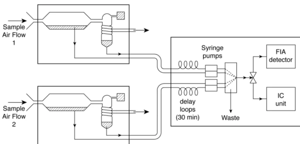
The GRAEGOR (Thomas et al., 2009) is a wet chemical instrument for semi-continuous, simultaneous two-point concentration measurements of water-soluble re-active trace gases (NH3, HNO3, HONO, HCl, and SO2) and their related particulate

10

compounds (NH+₄, NO−₃, Cl−, SO2₄−). GRAEGOR collects the gas and particulate sam-ples simultaneously at two heights using horizontally aligned wet-annular rotating de-nuders and steam-jet aerosol collectors (SJAC), respectively (see to Fig. 1). Air is simultaneously drawn through the sample boxes, passing first the wet-annular rotating denuders, where water-soluble gases diffuse from a laminar air stream into the sample

15

liquid. In both SJACs, the sample air is then mixed with water vapour from double-de-ionized water and the supersaturation causes particles to grow rapidly (within 0.1 s) into droplets of at least 2 µm diameter. These droplets, containing the dissolved particulate species are then collected in a cyclone (cf. Trebs et al., 2004). The airflow through the two sample boxes is∼14 L min−1 (at STP=0◦C and 1013.25 hPa) per box and is kept

20

constant by a critical orifice downstream of the SJAC. Liquid samples are sequentially analyzed online using ion chromatography (IC) for anions and flow injection analysis (FIA) for NH3and particulate NH+4. Within each full hour GRAEGOR provides one half-hourly integrated gas and particulate concentration for each height for each species (one sequential analytical cycle of all four liquid samples (two denuder, two SJAC

sam-25

ples) takes 1 h, cf. Thomas et al., 2009).

(8)

AMTD

2, 2423–2482, 2009

flux errors

V. Wolffet al.

Title Page

Tables Figures

◭ ◮

Back Close

Full Screen / Esc

et al., 2004). Prior to analysis an internal bromide standard is added to each sample. Additionally to its use in the determination of the concentration value, it is used in combination with monitoring the FIA waste flow as an internal quality indicator, enabling the identification of poor chromatograms (high/noisy baseline, bad peak shapes), high double-de-ionized water conductivity and unstable flows.

5

During NitroEurope (NEU) the inlets of the sample boxes, directly connected to the wet-annular rotating denuders, consisted of PFA (perflouroalkoxy) Teflon tubing (I.D.=0.8 cm, length=30 cm), ending upstream in a PE-funnel covered by a mosquito net. NEU measurements were made in the middle of an intensively managed plot, and, according to the available fetch (Ammann et al., 2007; Neftel et al., 2008),

mea-10

surement heights were chosen to be 1.23 and 0.37 m above ground. During EGER, measurements were performed on a walk-up tower and the sample boxes were located on 24.4 and 30.9 m above ground. The PFA Teflon tubing inlets of the sample boxes were shortened in comparison to the NEU arrangement (I.D.=0.8 cm, length=20 cm) and a PFA Teflon gauze (instead of the mosquito net) was placed inside a home-made

15

PFA Teflon rain protection.

2.1.4 Calibration and errors of the concentration measurements

The FIA cell was calibrated using liquid standards once a week, while the IC response was checked with liquid standards once or twice during each experiment. Field blanks representing the zero concentration signal of the system were measured once a week

20

by switching offthe sampling pumps and sealing the inlets, leaving the rest of the sys-tem unchanged (see Thomas et al., 2009). The random error of the measured air concentrations of NH3, HNO3, NH+4 and NO

−

3 was calculated according to Trebs et al. (2004) and Thomas et al. (2009) using Gaussian error propagation. The concentration error depends on the individual random errors of the sample airflow, the liquid sample

25

(9)

AMTD

2, 2423–2482, 2009

flux errors

V. Wolffet al.

Title Page

Tables Figures

◭ ◮

Back Close

Full Screen / Esc

performance, but also by (a) measuring the air flow through the sample boxes with an independent device (Gilibrator, Gilian, Sensodyne) once per day and (b) measuring and adjusting the liquid flow supply of the SJAC once per week. Additionally, other factors may affect the sample efficiency of the sample boxes. Therefore, the coating of the denuders was visually checked at least once per day and also the inlets were

5

checked every day for visible contamination and water droplets.

2.1.5 Determination of the concentration di_fference error

Evaluating potential error sources of the concentrations measured by GRAEGOR, it is obvious that some of them (e.g., the error of the bromide standard, see Sect. 2.2.2) do not influence the error of the difference between the concentrations, σ_∆_C, sampled by

10

the two individual sampling boxes because the same analytical unit and the same stan-dard solutions are used for deriving both concentrations. Some of the error sources of an individual concentration value are, however, relevant for∆C, as they may theoret-ically impact the concentrations at the two heights differently (e.g. the airflow through the sample boxes and the liquid flows). Additionally, other factors may introduce

dif-15

ferent sample efficiency of the sample boxes and thus impact on the precision of ∆C. Thus, the determination ofσ_∆_C is not to be performed straight forward from the error in concentrations.

Some of the factors lead to random errors, i.e. to a scatter in both directions around a “true value”, whereas some of them may lead to temporal or non-temporal systematic

20

errors, such as constant different sampling efficiencies. In order to investigate and characterize these errors, we performed extended side-by-side measurements during our field experiments, as integrated error analysis for ∆C. The sample boxes were regularly placed side-by-side during time periods of different length, but totally of 352 h (NEU) and of 255 h (EGER). During NEU, sampling could be performed through one

25

(10)

AMTD

2, 2423–2482, 2009

flux errors

V. Wolffet al.

Title Page

Tables Figures

◭ ◮

Back Close

Full Screen / Esc

measurement periods were performed, while during EGER, due the difficult set up at the tower, we confined ourselves to two side-by-side measurement periods at the beginning and the end of the experiment.

We plotted the concentrations measured with the two sample boxes side-by-side against each other and made an orthogonal fit through the scatter plots by minimizing

5

the perpendicular distances from the data to the fitted line. That way, both concentra-tion values are treated the same way, taking into account that both concentraconcentra-tions may be prone to measurement errors. We define a consistent deviation from the 1:1 line as systematic difference between the concentration measurements and we correct for it applying the calculated fit-equation. We regard the remaining scatter around the fit as

10

random error between the concentration measurements of the two boxes.

2.2 The aerodynamic gradient method (AGM)

Applying the AGM the turbulent vertical transport of an entity towards to or away from the surface is, in analogy to Fick’s first law, considered as the product of the turbulent diffusion (transfer) coefficient and the vertical air concentration gradient ∂C/∂z in the

15

so-called constant flux layer (Foken, 2006).

FC =−KH(u∗, z, L)·

∂C

∂z (1)

Usually, the turbulent diffusion coefficients for scalars (sensible heat, water vapour, trace compounds) are assumed to be equal (Foken, 2006). The turbulent diffusion coefficient for sensible heat, KH, expresses both, the mechanic turbulence, induced

20

by friction shear (expressed through the friction velocity, u_∗) and the thermal turbu-lence induced by the thermal stability of the atmosphere (expressed inz/L). It is thus a function of the height z (m) above the zero plane displacement height d (m), and atmospheric stability, parameterized by the Monin-Obukhov lengthL(m):

L=− u

3

∗

κ· g_T · _ρH_·_c

p

(2)

(11)

AMTD

2, 2423–2482, 2009

flux errors

V. Wolffet al.

Title Page

Tables Figures

◭ ◮

Back Close

Full Screen / Esc

where u_∗ is the friction velocity (m s−1), g the acceleration of gravity (m s−2), T the (absolute) air temperature (K), H the turbulent sensible heat flux (W m−2), ρ the air density (kg m−3),cpthe specific heat of air at constant pressure, andκthe von Karman constant (0.4) (Arya, 2001). H and u_∗ are usually measured by the eddy-covariance technique (or derived from gradient measurements of the vertical gradients of wind

5

speed and air temperature; Garratt, 1992).

For practical reasons, the flux-gradient relationship is usually not applied in the diff er-ential form (Eq. 1) but in an integral form between two measurement heights,z1andz2 (in m); accordingly the flux is derived from the difference in concentration,∆C=C2−C1 (in µg m−3), measured at the two heights, as (Mueller et al., 1993):

10

FC =−

u_∗·κ

lnz2 z₁

−ΨH _z

2 L

+ ΨH _z

1 L

| {z }

=v_tr

·∆C (3)

withκ the von Karman constant (0.4) andΨH, the integrated stability correction func-tion for sensible heat (equal to that of trace compounds). The left term of the product on the right hand side of Eq. (3) is often referred to as the transfer velocity,v_tr (m s−1). It represents the inverse resistance of the turbulent transport between the two heights

15

z1 and z2 (Ammann, 1998). Note here, that we use all measurement heights z1, z2, andz, as aerodynamic heights above the zero plane displacement height,d. For the grassland site (NEU) with varying canopy heighthcanopy,d (in m above ground) was estimated asd=0.66·(hcanopy−0.06) according to Neftel et al. (2007), and for the forest site (with constant canopy height during our study) it was determined as 14 m above

20

ground (Thomas and Foken, 2007).

When applying the AGM the accurate measurement of the concentration difference of the substance of interest is the major challenge. This is especially the case in remote environments, where concentrations are very low (Wesely and Hicks, 2000) and vertical concentration differences are in the order of 1 to 20% of the mean concentration

(12)

AMTD

2, 2423–2482, 2009

flux errors

V. Wolffet al.

Title Page

Tables Figures

◭ ◮

Back Close

Full Screen / Esc

(Businger, 1986; Foken, 2006).

2.3 Flux error analysis

When applying the AGM for measurements of two point vertical concentration diff er-ences, the flux is determined from the product of∆Cand vtr (see Eq. 3). A flux error thus includes the errors of factors,σ_∆_C andσ_v

tr.σ∆C is derived from side-by-side

mea-5

surements as described in Sect. 2.2.3. σv_tr will be estimated from errors of the main influencing parameters ofvtr as described in Sect. 4.4.

These two errors, σ_∆_C and σ_v

tr, have different effects on the resulting flux, its sign, magnitude and error. The sign of∆Cdetermines the sign and therefore the direction of the derived flux. Thus, σ_∆_C is a measure of the significance of the derived flux

10

direction, additionally to the influence ofσ_∆_C on the magnitude of the flux error. The error ofvtrhowever, expresses the uncertainty in the velocity of exchange and therefore influences the magnitude of the flux error, butσ_v_tr does not impact the significance of the flux sign. Fromσ_∆_C we can deduce the significance of a difference from zero and subsequently of the flux direction. The error of the flux,σF, we deduce by combining

15

the two values,σ_∆_C andσ_v_tr, using Gaussian error propagation:

σF =F · s

_σ v_tr

vtr 2

+

_σ ∆C

∆C

2

(4)

3 Constraints for the precision – theoretical approach

To obtain an estimate of the precision required to resolve vertical concentration gradi-ents with regard to stability and measurement heights using Eq. (3), an independent

20

(13)

AMTD

2, 2423–2482, 2009

flux errors

V. Wolffet al.

Title Page Abstract Introduction Conclusions References Tables Figures ◭ ◮ ◭ ◮ Back Close

Full Screen / Esc

multiple resistance approach” (Wesely and Hicks, 2000; Hicks et al., 1987). In analogy to Ohm’s law, the flux of HNO₃ is expressed as the ratio of the HNO₃ concentration,

CHNO₃ at one height and the resistances against deposition to the ground. This resis-tance consists of three individual resisresis-tancesR_a,R_b, andR_c, each of them character-izing part of the deposition process:

5

FHNO₃ =−

1

R_a+R_b+R_c ·CHNO3 (5)

withFHNO₃ denoting the HNO3 deposition flux (µg m

−2

s−1),Rathe aerodynamic resis-tance (s m−1), R_b the quasi-laminar or viscous boundary layer resistance (s m−1), R_c

the surface resistance (s m−1) and CHNO₃ the concentration of HNO3 (µg m− 3

). R_a is calculated according to Garland (1977). It is defined for a measurement heightz (m)

10

above a surface of roughness lengthz0(m):

Ra(z, z0)= 1

κ·u_∗

ln z z0

−ΨH _z

L

(6)

The roughness length, z0, of the grassland site was derived from wind and tur-bulence measurements (Neftel et al., 2007) as a function of the canopy height:

z0=0.25·(hcanopy−d). Wind profile analysis for the forest site revealed a value of z0

15

of 2 m (Thomas and Foken, 2007). R_b determines the exchange immediately above the vegetation elements and can be described by (Hicks et al., 1987):

R_b=_κ2 ·u_∗

Sc Pr

2₃

(7)

where Sc and Pr are the Schmidt and Prandtl number (≈0.72), respectively. Sc is a strong function of the molecular diffusivity of the trace gas (for HNO3≈1.25) (Hicks et

20

(14)

AMTD

2, 2423–2482, 2009

flux errors

V. Wolffet al.

Full Screen / Esc

2001; Hanson and Lindberg, 1991) and thus, the theoretical maximum deposition flux of HNO₃towards the surface can be obtained by:

Fmax_HNO3 =− 1

R_a+R_b·CHNO3 (8)

This maximum HNO3flux value (calculated withC2at heightz2) will be used to estimate the minimal requirements which the instrument’s precision must satisfy to determine

5

fluxes with the AGM at the two sites for a range of atmospheric stabilities.

3.1 Influence of atmospheric stability

Combining Eqs. (3) and (8) we may calculate a maximum possible concentration dif-ference for the maximum HNO3deposition flux (Rc=0)

∆Cmax=

CHNO₃· h

lnz2 z₁

−ΨH _z

2 L

+ ΨH _z

1 L

i

κ·u_∗·[Ra(z, z0)+Rb]

(9)

10

Including Eqs. (6) and (7) and solving the equation for the maximum concentration difference relative to the HNO3concentration, we obtain:

∆C_max CHNO₃

=

lnz2 z₁

−ΨH _z

2 L

+ ΨH _z

1 L

lnz2 z₀

−ΨH _z

2 L

+2·Sc Pr

2 3

(10)

Equation (10) provides a minimal requirement for the instrument precision to resolve vertical concentration differences as a function of the aerodynamic stability (z/L), the

15

(15)

AMTD

2, 2423–2482, 2009

flux errors

V. Wolffet al.

Title Page

Tables Figures

◭ ◮

Back Close

Full Screen / Esc

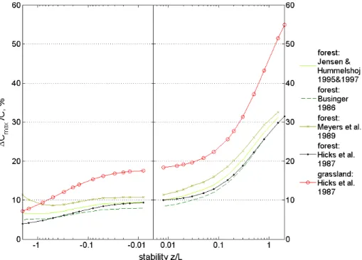
We have calculated ∆Cmax/C for a range of stabilities using the roughness length (z0) and the measurement heights of the two sites using different parameterisations for

R_b(Fig. 2). ∆C_max/C depends to a large extend on the atmospheric stability, ranging from 55% at the grassland site for extremely stable conditions (32% at the forest site) to less than 10% at the grassland (around 5% at the forest site) for labile conditions.

5

Higher roughness at the forest site (EGER) leads to generally lower∆Cmax/Cvalues for all stabilities compared to the grassland site.

3.2 Influence of the measurement heights

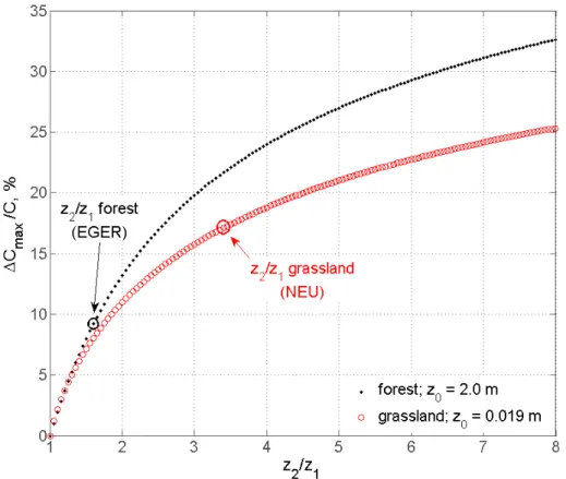
The influence of the measurement heights above the surface on the minimal precision requirements is also estimated from Eq. (10). For near neutral conditions, whenz/Lis

10

close to zero,ΨHis close to zero such that we may simplify Eq. (10) to:

∆Cmax

CHNO₃

=

lnz2 z1

lnz2 z₀

+2·Sc_Pr

2 3

(11)

The second term in the denominator is a constant derived fromR_b, which has a bigger influence on∆C_max/Cabove a forest than above grassland, where ln(z₂/z₀) is smaller.

∆Cmax/Cincreases with increasing z2/z1 values (Fig. 3), thus the precision

require-15

ments decrease with increasing measurement height ratios. There are, however, re-strictions to the choice of measurement heights. The upper measurement height must be chosen according to fetch limitations, i.e. the uniform fetch length must be larger than one hundred times the measurement height (e.g. Businger, 1986). Above forests, the tower height and the sensor accessibility are additional limiting factors. In turn, the

20

(16)

AMTD

2, 2423–2482, 2009

flux errors

V. Wolffet al.

Title Page

Tables Figures

◭ ◮

Back Close

Full Screen / Esc

EGER), respectively.

Above rough surfaces, such as forest canopies, deviations from the ideal flux-gradient relationship used here are frequently observed within the so-called rough-ness sublayer, which may extend up to two times the canopy height (Foken, 2006). In this layer the use of flux gradient relations may underestimate scalar fluxes by 10% or

5

more (Simpson et al., 1998; Thom et al., 1975; Hogstrom, 1990; Garratt, 1978; Cel-lier and Brunet, 1992). Therefore the detection limits for EGER derived here have to be considered as rough estimates. A detailed analysis of the site-specific flux-profile relationships above the forest (derived for non-reactive trace gases) will be published elsewhere.

10

4 Experimental results

4.1 Overview

The determined random error of the measured air concentrations, determined after Trebs et al. (2004) and Thomas et al. (2009), was in the order of 10%. Note here, that only individual quantifiable error sources are included in this error estimation. Errors in

15

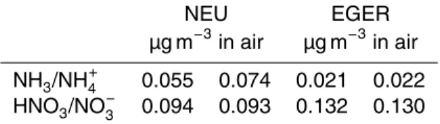
concentration values that are not quantifiable, e.g. errors due to limited sampling effi -ciency, may only be investigated by differential analysis, like the side-by-side measure-ments (see Sects. 2.2.3 and 4.2). The limit of detection (LOD) under field conditions was determined as three times the standard deviation of the blank values (Kaiser and Specker, 1956) and results are summarized in Table 1. During NEU, problems with the

20

membrane in the FIA and sensor damage in the course of the experiment increased the LOD of the NH3/NH+4-measurement.

Concentration values below the detection limit were used in the general time se-ries analysis, but data points were flagged and their error (σ_C/C) was set to 100%. However, for the side-by-side evaluation they were excluded. Furthermore, data points

25

(17)

AMTD

2, 2423–2482, 2009

flux errors

V. Wolffet al.

Title Page

Tables Figures

◭ ◮

Back Close

Full Screen / Esc

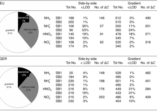
and liquid flow stability and obvious contamination (e.g. after manual air flow measure-ment). An outlier test was performed according to Vickers and Mahrt (1997) and the respective values were excluded from analysis. The overall data availability during the experiments is shown in Table 2. Roughly 10% of the measurement period was used for calibrations and blanks. One third was used for side-by-side measurements and

5

two thirds of the measurement period the instrument measured concentration at two different heights.

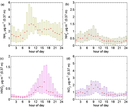
4.2 Diel variation of concentrations and aerodynamic parameters

Diel variations of the concentrations measured during the experiments are presented in Fig. 4 (NEU) and Fig. 5 (EGER) as median, 0.25 and 0.75 percentiles. During NEU,

10

NH3concentrations atz=0.37 m (above ground) (median values: 1.24 to 3 µg m− 3

) ex-ceeded concentrations of all other compounds by a factor of 2 to 4 and were higher than those observed during EGER (median values: 0.46 to 1.16 µg m−3). During NEU, NH3concentrations featured a sharp peak during the morning hours, while NH3peaked in the afternoon/late afternoon hours during EGER. Concentrations of particulate NH+₄

15

were twice as high during EGER (median values: 0.9 to 1.44 µg m−3) compared to NEU (median values: 0.31 to 0.77 µg m−3). During both campaigns, particulate NH+₄ exhibited a diel variation with higher concentrations during nighttime and lower con-centrations during daytime. HNO3 concentration levels were similar during NEU and EGER with median values between 0.2 and 0.7 µg m−3. No significant diel variation

20

of HNO₃ was observed above the forest during EGER while HNO₃ featured a typical diel cycle with broad maxima in the afternoon during NEU. Particulate NO−₃ concentra-tions were much larger during EGER than during NEU, with median values between 1.8 and 3 µg m−3. Although, the variation of particulate NO−₃ was smaller during EGER than during NEU, it typically showed highest values during nighttime and/or in the early

25

morning hours.

(18)

high-AMTD

2, 2423–2482, 2009

flux errors

V. Wolffet al.

Title Page

Tables Figures

◭ ◮

Back Close

Full Screen / Esc

est values during the day (Fig. 6).z/Lranged from−0.25 to 0.3, indicating stable con-ditions at night and unstable and near neutral concon-ditions during the day. During EGER,

u_∗ was much higher with values between 0.25 and 0.8 m s−1 and z/L was between

−0.3 and 0.5, also indicating stable conditions during nighttime and neutral/unstable conditions during daytime.

5

A detailed analysis of the data acquired during NEU and EGER including gas-particle interactions and flux interpretations will be performed in subsequent publications.

4.3 Error of∆Cdetermined from side-by-side measurements

To estimate the effective error of∆C(σ_∆C) under field conditions, we used results from extended side-by-side sampling periods during both experiments. The weather

condi-10

tions and ambient concentrations of the compounds under study were similar during side-by-side and aerodynamic gradient measurements. Results from the side-by-side measurements are displayed as scatter plots in Figs. 7 and 8 for NEU and for EGER, respectively. Concentrations sampled during rain events and during episodes with high relative humidity (>95%) are excluded from the side-by-side evaluation and from the

15

flux determinations, since during these times adsorption processes in the humid in-let and potential contamination of the denuder by water dropin-lets can not entirely be excluded.

Figures 7 and 8 show marked linear correlations between concentrations measured by the two sample boxes, however, deviations from the 1:1 line and scatter around

20

the fitted lines is visible. HNO₃ side-by-side measurements featured slopes with lit-tle deviation from the 1:1 line (1.01 and 1.02 for NEU and EGER, respectively) and small offsets. Side-by-side measurements for NH3 during NEU (Fig. 7a) also featured a slope close to unity (slope: 0.93). During EGER (Fig. 8a), under much lower NH₃ concentrations, the deviation from the 1:1 line was somewhat larger (1.13), whereas

25

(19)

AMTD

2, 2423–2482, 2009

flux errors

V. Wolffet al.

Title Page

Tables Figures

◭ ◮

Back Close

Full Screen / Esc

a slope of 1.59 in the NEU experiment and 1.31 in the EGER experiment.

After we corrected the data using the orthogonal fit (systematic deviation, see above), the remaining scatter around the fit (the residuals) was used to determine

σ_∆C. Figure 9 shows exemplarily two typical residual distributions.

The histograms of the residuals show a pronounced peak around zero with a steep

5

decrease of the relative frequency and pronounced tails towards both directions (in-creasing residuals of∆C). These distributions follow more closely a Laplace (or dou-ble exponential) distribution than a Gaussian distribution, as it was also observed for errors in the measurements of other atmospheric quantities (Richardson et al., 2006). In contrast to the usual Gaussian distribution, the standard deviation (1std) of values

10

following the Laplace distribution is determined as:

stdLaplace = p

2·

N P

i=1

|xi−x|¯

n (12)

withndenoting the total number of values within the distribution, ¯x the mean, andx_i all residual values, which encompass 76% of the Laplace distribution (which corresponds to 68.27% in the Gaussian distribution, analogously, 2std correspond to 95.45% of

15

a Gaussian distribution, but to 94% of a Laplace distribution; see Richardson et al., 2006).

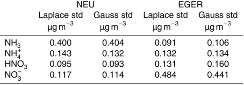
The distributions of concentration residuals provide valuable information on the be-haviour of the instrument. The width of the residual distribution characterizes the random concentration difference during side-by-side measurements in the field. The

20

Laplace standard deviations for each of the compounds are given in Table 3 for the two experiments. For comparison, the standard deviations calculated for the Gaussian distribution are also shown.

For NH₃, HNO₃ and NO−₃ during NEU and NH₃, NH+₄ and HNO₃ during EGER, we observed increasing std_∆C values with increasingC. Therefore, we plotted std∆C vs.C

25

(20)

AMTD

2, 2423–2482, 2009

flux errors

V. Wolffet al.

Title Page

Tables Figures

◭ ◮

Back Close

Full Screen / Esc

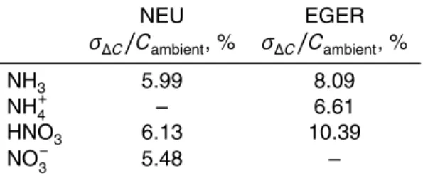
used to determine std_∆C as a function ofC. The relative values std∆C/Cderived from the slopes of the regressions, which are used as estimates of σ_∆_C, are summarized in Table 4. For particulate NH+₄ during NEU and for particulate NO−₃ during EGER, this approach did not appear to be useful, because the residuals did not show a clear dependence on C in these cases. Hence, we defined the overall Laplace standard

5

deviation (Table 3) as the errorσ_∆_C. Median relative determined errors (σ_∆_C/∆C) were 36.3 and 55.5% for NH₃, 40.1 and 59.4% for HNO₃, 129.6 and 63.3% for particulate NH+₄ and 49.4 and 244% for particulate NO−₃ during NEU and EGER, respectively.

The resultingσ_∆_C values may be used for two purposes: (a) to describe an uncer-tainty range around zero, and thus give an estimate about the precision of the gradient

10

system at a given concentration, and (b) to determine the significance of a measured

∆C value for flux calculations. ∆C values inside the uncertainty range around zero carry error bars that are larger than∆Citself and it is not possible to derive significant fluxes from these∆Cvalues, nor meaningful deposition velocities.

We define those∆Cvalues as insignificantly different from zero. Results of this

anal-15

ysis for some days of the EGER experiment are displayed in Fig. 12. In cases when the uncertainty range is a function of concentration, the diel variation of concentrations is reflected in the size of the error bars and uncertainty ranges (grey bars). For exam-ple, for NH₃ concentrations during EGER error bars are larger during daytime when NH3concentrations are high (Fig. 12a). For the days shown here, both, significant and

20

non-significant∆Cvalues are observed.

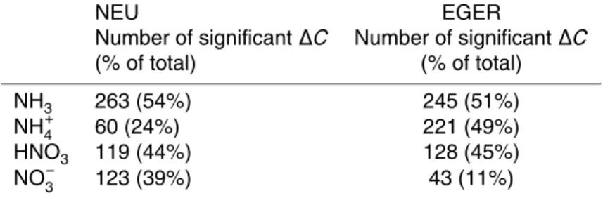
From the relative values,σ_∆C/C, in Table 4 we define an uncertainty range around zero and therefore a significance level for ∆C for the given ambient concentration. Between 11 to 54% of the individual∆Cvalues, determined from aerodynamic gradient measurements, during EGER and NEU are found to be significantly different from zero

25

(21)

AMTD

2, 2423–2482, 2009

flux errors

V. Wolffet al.

Full Screen / Esc

Interactive Discussion 4.4 Error of the transfer velocity

Since the exchange flux of the considered trace gases is defined as the product of∆C

and vtr we also need to investigate σv_tr. As stated above, vtr is a function of u∗, and,

in the denominator, ln(z2/z1) and the integrated stability correction functions for heat (=trace compounds) for both measurement heights (ΨH(z1/L) andΨH(z2/L)), which

5

are (via the Monin-Obukhov length, Eq. 2) a function ofu_∗, the sensible heat flux (H), a buoyancy parameter (g/T), the air density (ρ), the von Karman constant and the specific heat (cp) (e.g., Arya 2001).

A complete error analysis ofvtr would require information about the error of all these parameters. We have not found any study, which has thoroughly quantifiedσ_v

tr. Since

10

a detailed analysis ofσv_tr is not the main scope of this study, we use a simplified ap-proach to estimate this value. A first simple apap-proach is to scale the error of the trans-fer velocity with the error of u_∗, especially under near-neutral conditions, when the integrated empirical functions in the denominator of Eq. (3) approach unity. For the sonic anemometer used during our studies, the error ofu_∗can be estimated as≤10%

15

(Foken, 2006). This relative error would directly propagate tovtr.

For non-neutral conditions, error estimates of the empirical functions within the sta-bility range of−0.5≤z/L≤+0.5 exist (Foken, 2006). Assuming that the errors remain the same when integrating the empirical functions the errors would also be in the range of≤10%. Assuming near-normal distribution of bothσu_∗andσΨH,σv_tr can be calculated

20

according to:

σ_v_tr vtr =± v u u u u t _σ u∗ u_∗ 2 + _σ ΨH ΨH 2 ·   

(ΨH(z2)+ ΨH(z1))2

lnz2 z₁

−ΨH(z2)+ ΨH(z1) 2





 (13)

The right hand term of the product under the square root accounts for the fact that in Eq. (3) twoΨHfunctions appear in the denominator. Note that we assume a maximum relative error of bothΨHfunctions (10%). The errors ofu∗andΨHadd up to a daytime

(22)

AMTD

2, 2423–2482, 2009

flux errors

V. Wolffet al.

Title Page

Tables Figures

◭ ◮

Back Close

Full Screen / Esc

(−0.5≤z/L≤+0.5) σv_tr/vtr of around 10% (median) during NEU (inter-quartile range: 10.1–13.3%) and 13% (median) during EGER (inter-quartile range: 10.3–23.2%). Note that for smallu_∗ values, the assumption of a constant relative error may not be appro-priate.

4.5 Flux error 5

In the previous sections we have determined σ_∆_C/C and we also obtained an error estimate for σ_v

tr/vtr. We combine these relative errors and derive the flux error, σF, applying Eq. (4). The resultingσFare presented along with determined fluxes in Fig. 13 for some days during EGER.

Most of the timeσ_F is primarily governed byσ_∆_C, but on the 22 and 23 September,

10

largeσv_tr values dominateσF during daytime. The overallσF during EGER would de-crease by 4% (median, inter-quartile range: 2–10%) if we exclude σ_v_tr and use σ_∆_C

only. During NEU, the error would decrease by 2% (median, inter-quartile range: 1– 4%). It is evident that,σF depends to a major extent on the capability of the instrument to precisely resolve vertical concentration differences.

15

The statistical distribution of flux errors relative to the determined flux values (σF/F) for∆Cvalues larger thanσ_∆C are presented in Fig. 14 for NEU and Fig. 15 for EGER. Medians ofσF/F vary between 31 and 68%. The values are comparable for all com-pounds, but show slightly larger ranges and higher medians for NH+₄ during NEU and NO−₃ during EGER

20

5 Discussion

5.1 Side-by-side performance of the GREAGOR system

(23)

AMTD

2, 2423–2482, 2009

flux errors

V. Wolffet al.

Title Page

Tables Figures

◭ ◮

Back Close

Full Screen / Esc

on∆C, but others do. The error of the peak integration, which affects the measured liquid concentration and the measured bromide concentration (cf. Trebs et al., 2004), for example, is relevant for∆Cas these errors may vary during the sequential runs of the ion chromatograph. Additionally, the two airflows though the sample boxes may have slightly different variations since the two critical orifices are not entirely identical.

5

There are also some other factors that may affect∆Cwhich are hard to quantify and to monitor. The wet-annular rotating denuder walls may not always be perfectly coated, and the liquid levels, controlled by optical sensors, may be slightly different between the two wet-annular rotating denuders. The difference in coating quality would lead to slightly different sampling efficiencies between the two heights, especially if the coating

10

is not perfect in the first part of the denuder (Thomas et al., 2009). The difference in water level results in a different response time of the instrument, leading to a damp-ening of concentration variations in the potentially affected denuder (Thomas et al., 2009). ∆C may also be influenced by inlet effects of the two sample boxes. Due to their high solubility and high surface affinity, HNO3 and NH3 may be lost in the inlet,

15

especially under very humid conditions. To minimize these effects we used short PFA tubing and treat measurement values from periods with rain and high relative humidity with caution. This, however, may not fully exclude different behaviour of the two inlets.

The discussed error sources have different effects on the sampled species, which is most evident for particulate NH+₄. Sorooshian et al. (2006) showed that

particu-20

late NH+₄ is most vulnerable to evaporational loss within the condensation chamber of the PILS (particle into liquid sampler), whose principle of operation is comparable to the SJAC. They showed that the particulate NH+₄ sampling efficiency is dependent on the temperature of the water vapour, the pH of the sampled particulate, and the dilu-tion. Particulate NH+₄ evaporation increases (and is therefore lost within the sample)

25

(24)

ob-AMTD

2, 2423–2482, 2009

flux errors

V. Wolffet al.

Title Page

Tables Figures

◭ ◮

Back Close

Full Screen / Esc

served for concentrations below 2.5 µg m−3. The deviation of up to 59% (Figs. 7 and 8) between the two sample boxes, suggest that the SJAC sampling efficiency was not equal for the two devices. For the NEU experiment, NH+₄ concentrations were quite low (up to 2 µg m−3; compared to 14 µg m−3 in Thomas et al., 2009) and regression was calculated for a number of only 17 data pairs. This may explain the somewhat poor

5

side-by-side results for NH+₄ during NEU (Fig. 7).

We were not able to clarify the reasons for this behaviour yet, but since the diff er-ences proved to be quite stable during both experiments, we were able to correct for this systematic difference (cf. Sect. 2.2.3).

5.2 Comparison to previous studies 10

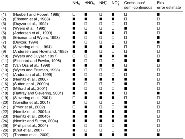
5.2.1 Overview of NH3-HNO3-NH4NO3aerodynamic gradient measurements

Table 6 shows a list of studies that have measured and investigated vertical con-centration gradients of NH3, HNO3 and particulate NH+4/NO

−

3 to determine surface-atmosphere exchange fluxes over different ecosystems.

The studies with non-continuous or semi-continuous measurements were performed

15

with denuders or filter-packs and measured integrated replicates at every measure-ment height. Corresponding concentration data, i.e. means and standard deviations, were then used to distinguish significant from insignificant∆C. In some studies pre-cision analysis was performed by individual side-by-side measurements of denuders or filter-packs (e.g., Huebert and Robert, 1985). Resulting errors of the exchange

20

fluxes were often only qualitatively discussed (e.g., Duyzer, 1994). Fifteen out of the twenty-eight studies made continuous or semi-continuous measurements of at least one compound in the triad (e.g. study 4, 10, and 11, Table 6), even less made mea-surements of the complete NH₃-HNO₃-NH₄NO₃ triad (studies 15, 22–24 and 27, Ta-ble 6). Methods with a higher temporal resolution than the GRAEGOR can make use

25

(25)

AMTD

2, 2423–2482, 2009

flux errors

V. Wolffet al.

Title Page

Tables Figures

◭ ◮

Back Close

Full Screen / Esc

errors (Flechard and Fowler, 1998). In contrast, a precision analysis of aerodynamic gradient measurements with longer sampling periods (e.g. 30 min like GRAEGOR) has to be performed differently, because only one concentration measurement per height per half an hour is available. Wyers et al. (1992), Wyers et al. (1993), and Kruit et al. (2007) demonstrated the use of side-by-side measurements to estimate the precision

5

of their semi-continuous NH3 aerodynamic gradient measurements. They called de-viations from the 1:1 line systematic differences and corrected for them; the standard deviation of the remaining scatter was used as an estimate of measurement noise. Many of the remaining studies do not show error estimates of their derived fluxes and deposition velocities. So far, only Thomas et al. (2009) feature a precision analysis for

10

the whole NH₃-HNO₃-NH₄NO₃triad.

5.2.2 Error of concentration differences

About 49% of∆C data for NH3 during EGER were found to be not significantly diff er-ent from zero (Table 5). Keeping in mind that measuremer-ents were performed above forest with the expected small∆Cvalues (Fig. 3), a 51% yield of significant half hourly

15

aerodynamic gradient measurements is satisfying. Andersen et al. (1993), who mea-sured NH3 exchange with three hourly-integrated denuder measurements on several levels above forest, were able to use less than half of the measurements for flux calcu-lations. Wet-chemical semi-continuous methods comparable to GRAEGOR, for which the precision to resolve vertical concentration differences was determined have been

20

presented by Wyers et al. (1993), Kruit et al. (2007), and Thomas et al. (2009). Wyers et al. tested their NH3 gradient system (AMANDA: based on three wet-annular de-nuders coupled to one flow injection analytical unit) for precision by side-by-side mea-surements. They reported average relative standard deviation of 1.9% of 42 triplicate measurements. However, they did not give any information whether these tests were

25

(26)

AMTD

2, 2423–2482, 2009

flux errors

V. Wolffet al.

Title Page

Tables Figures

◭ ◮

Back Close

Full Screen / Esc

wet-annular denuders and one flow injection analytical unit. Improvements compared to AMANDA were a stabilized liquid flow and monitoring of the air flow through the denuders. They tested their system under laboratory conditions, feeding the three wet-annular rotating denuders simultaneously with two different standard NH3 concen-trations (0 and 8 µg m−3) over five hours and corrected for the deviations between the

5

samples in the same way as Wyers et al. (1993) (see Sect. 4.1.1). From these tests, they conclude that their precision was at least as good as found by Wyers et al. (1993), if not better (<1.9%). However, these tests do neither take into account the behaviour of the measurement system and analytical unit under ambient conditions nor the dy-namic changes of ambient concentrations and associated fluctuations of temperature

10

and relative humidity during field experiments.

In 2009, Thomas et al. introduced the GRAEGOR instrument and investigated its precision by performing a side-by-side experiment in the field under ambient condi-tions. They calculated linear regressions through the concentration data and used the deviation of the derived slope from the 1:1 line as their precision. They found 3% for

15

gases and 9% for particulate compounds. The use of the deviation from the 1:1 line as precision estimate (not taking into account the scatter around it) is different to the methods used by Wyers et al. (1993) and Kruit et al. (2007), who defined this a sys-tematic error and derived their random error from the remaining scatter. However, the approach by Thomas et al. was a first attempt to estimate the instrument precision for

20

aerodynamic gradient measurements. Thomas et al. (2009) also defined their mini-mum detectable flux whenσ_∆_C equals∆C, but they did not take into account the error of the transfer velocity. Side-by-side measurements by Thomas et al. (2009) featured smaller systematic deviations from the 1:1 line than found in our study. Concentration ranges for NH3, HNO3 and NO−3 are comparable to the ones observed in our

exper-25

(27)

influ-AMTD

2, 2423–2482, 2009

flux errors

V. Wolffet al.

Title Page

Tables Figures

◭ ◮

Back Close

Full Screen / Esc

enced by environmental conditions (see Sect. 5.1). An analysis of the Thomas et al. side-by-side data with our method results in σ_∆C/C median values of 4.5% for NH3, 1.0% for NH+₄, 4.6% for HNO3, and 6.8% for NO−3. These values are lower than the ones found in our study (see Table 4) especially for particulate NH+₄, which however revealed much higher concentrations in Thomas et al. In this study, we combined the

5

approaches of Wyers et al. (1993), Kruit et al. (2007), and Thomas et al. (2009) by separating systematic from random effects using the scatter around the fitted line and by using side-by-side measurements in the field to account for the actual set up of the instrument and the environmental conditions encountered at the field sites. A diff er-ence to the previous studies is the use of an orthogonal fit rather than a least squares

10

regression to evaluate the side-by-side measurements. This fit takes into account that concentration measurements of both sample boxes may be erroneous, which is a more realistic approach than defining one of the measurements as independent (Hirsch and Gilroy, 1984; Ayers, 2001; Cantrell, 2008). The median σ_∆_C/∆C values range be-tween 36% (NH₃during NEU) and 244% (NO−₃ during EGER), see Sect. 4.2. Keeping

15

in mind, that the GRAEGOR is a semi-continuous measurement device, delivering all compounds of the triad (and more) in hourly resolution and that we use in-field data rather than laboratory test to express an in-field precision of the instrument, these pre-cision values are certainly satisfying.

5.2.3 Error of surface exchange fluxes 20

There are only six studies that show and discuss error bars of fluxes derived from measurements applying the AGM (see Table 6). Erismann and Wyers (1993) discussed in their study on SO2and NH3exchange fluxes above forest that the main error source for the NH3 flux and the NH3 canopy resistance error isσ∆C. They show data of NH3 fluxes and correspondingRc values with error bars of up to 100% and higher. They

25

(28)

AMTD

2, 2423–2482, 2009

flux errors

V. Wolffet al.

Title Page

Tables Figures

◭ ◮

Back Close

Full Screen / Esc

The same relative value is true for flux errors shown in a figure from Duyzer et al. (1994). All these errors do not includeσv_tr.

The relative flux errorsσF/F determined in our study, with medians between 31 and 68% (see Figs. 14 and 15), are comparable to these studies.

5.3 Influence of stability conditions on the precision 5

In Sect. 3.1 we investigated the expected magnitude of∆Cfor a range of atmospheric stabilities, assuming a maximum HNO₃ deposition flux. The precision requirement is higher for the forest site (EGER) with around 10% for near neutral and less than 10% for unstable conditions. These estimates depend to a major extend on the applied parameterisation forRb(see Fig. 2). Comparing these values with the relative precision

10

values given in Table 4 (EGER: right side) we see that for some species the precision may not be sufficient to determine significant∆C above the forest for all atmospheric stabilities.

For the grassland site (NEU), the required precision falls below 10% only at

z/L<−0.3. Thus, the determined precision values (left side Table 4) are sufficient

15

to determine significant ∆C for most atmospheric stabilities. Note, however, that the estimate presented in Sect. 3.1 is valid for a maximum deposition flux and that not all components measured here will always deposit with maximum velocity (R_c>0). Thus, the expected concentration differences may well be below the values given in Sect. 3.1 for compounds other than HNO3.

20

5.4 Influence of measurement height on the precision

It is evident from Sect. 3.2, which impact the choice of the measurement heights has on the required∆Cto be resolved. Knowing the relative precision of the instrument, for example 8% for NH3during EGER, minimalz2/z1ratios to resolve differences above a surface of given roughness can be calculated. However, as it was the case for the

25

(29)

micrometeoro-AMTD

2, 2423–2482, 2009

flux errors

V. Wolffet al.

Title Page

Tables Figures

◭ ◮

Back Close

Full Screen / Esc

logical considerations (such as uniform fetch length).

6 Conclusions

In this paper we made a comprehensive precision analysis for a novel wet-chemical in-strument used for aerodynamic gradient measurements of water-soluble reactive trace gases and particles (GRAEGOR; GRadient of Aerosol and Gases Online

Registra-5

tor; ECN, Petten, NL) with focus on the NH3-HNO3-NH4NO3 triad. For the first time, we present a thorough determination of errors of multi-component surface-atmosphere exchange fluxes for two contrasting ecosystems (managed grassland and spruce for-est). From our investigations, we draw conclusions on the significance of measured concentration differences and, thus, the direction and magnitude of multi-component

10

surface-atmosphere exchange fluxes.

Additionally, we investigated theoretical minimal precision requirements for surfaces with different roughness with regard to atmospheric stability and measurement heights, which may be used for future experimental designs, knowing the precision of the in-strument that will be used. Derived in-field precision values (σ_∆_C/C) of the instrument

15

during our field studies were 6% (NEU, grassland) and 8% (EGER, forest) for NH3, 6% (NEU) and 10% (EGER) for HNO₃, and 7% for particulate NH+₄ (EGER) and 5% for particulate NO−₃ (NEU). Thus, GRAEGOR is capable of resolving vertical concentra-tion differences of the four species under investigation above grassland and forest sites for most of the prevailing atmospheric stabilities. However, our analysis revealed that,

20

especially at the forest site, the precision of the instrument may not be sufficient to re-solve individual (hourly) gradients at labile atmospheric stability, even if the substance is deposited at maximum possible speed.

Despite the fact that GRAEGOR is operated using the same analytical device for both measurement heights the median error of the determined concentration difference

25

(30)

AMTD

2, 2423–2482, 2009

flux errors

V. Wolffet al.

Title Page

Tables Figures

◭ ◮

Back Close

Full Screen / Esc

limit of detection and side-by-side measurements under field conditions are a suitable tool to evaluate the instrument performance and to estimate the instrument precision and associated flux errors. The precision of GRAEGOR may be improved by intensive monitoring and controlling of error sources for aerodynamic gradient measurements like denuder liquid level and sample efficiency of the SJACs. We may assume that

5

errors in previous studies, where the aerodynamic gradient method was used to derive exchange fluxes of the NH3-HNO3-NH4NO3triad, were at least as high as during our study, especially if two different analytical devices were applied.

The instrument provides a semi-continuous data set, constituting valuable informa-tion for mechanistic process studies. Our results form the basis to explore the errors

10

of deposition velocities and canopy compensation point concentration, which are key-parameters used in all atmospheric chemistry and transport models. The results from the NEU and EGER campaigns will be discussed and interpreted in separate publica-tions.

Acknowledgements. The authors gratefully acknowledge financial support by the European

15

Commission (NitroEurope-IP, project 017841), the German Science foundation (DFG project EGER, ME 2100/4-1) and by the Max Planck Society. The authors wish to thank the Agroscope Reckenholz-T ¨anikon Research Station (ART, Air Pollution and Climate Research Group) for hosting us during the NitroEurope study and the University of Bayreuth (Micrometeorology Department) for hosting us during the EGER study.

20