www.hydrol-earth-syst-sci.net/13/27/2009/ © Author(s) 2009. This work is distributed under the Creative Commons Attribution 3.0 License.
Earth System
Sciences
Simulating typhoon-induced storm hydrographs in subtropical
mountainous watershed: an integrated 3-layer TOPMODEL
J.-C. Huang1, T.-Y. Lee1,2, and S.-J. Kao1,3
1Research Center for Environmental Changes, Academia Sinica, Taipei, Taiwan
2Department of Bioenvironmental Systems Engineering, National Taiwan University, Taipei, Taiwan 3State Key Laboratory of Marine Environmental Science, Xiamen University, Xiamen, China
Received: 20 February 2008 – Published in Hydrol. Earth Syst. Sci. Discuss.: 21 April 2008 Revised: 3 December 2008 – Accepted: 13 December 2008 – Published: 23 January 2009
Abstract.A three-layer TOPMODEL is constructed by inte-grating diffusion wave approach into surface flow, soil mois-ture deficit into inter flow and exponential recession curve function into base flow. A subtropical mountainous water-shed, Heng-Chi, and 22 rain storms with various rainfall types and wide ranges of total rainfall (from 81 to 1026 mm) were applied. The global best-fitted parameter set gives an average efficient coefficient of 82% for calibration and 80% for validation. Sensitivity analysis reveals that soil trans-missivity dominates the discharge volume and recession co-efficient dominates the hydrograph shape in TOPMODEL framework. Over 90% observed discharges of validation events falls within the 90% confidence interval derived form calibration events. The resembling performances between calibration and validation as well as good results of the con-fidence interval demonstrate the capability of 3-layer TOP-MODEL on simulating cyclones with various rainfall inten-sity and pattern in subtropical watershed. Meanwhile, the upper confidence limit is suggested preferably when consid-ering flood assessment.
1 Introduction
Taiwan, sitting on the Pacific Fault (orogenic belt), forested and precipitous landscape (mountainous area) occupies about 67% of the whole island. Meanwhile, the island also locates on the typhoon alley of the Western Pacific and it suffers frequent typhoons, about 3–5 typhoon in-vasions every summer (Taiwan Central Weather Bureau, www.cwb.gov.tw). Coupled with steep landscape and
frac-Correspondence to:S.-J. Kao ([email protected])
ture rocks, typhoon generally indicates debris flows and land-slides at the upstream and flood at downstream areas (Huang et al., 2007). For instances, Typhoon Herb in 1996, Zeb in 1998 and Xangsane in 2000 brought over 800 mm rainfall within two days. Typhoon Nari in 2001 broke the record by bringing 1026 mm rainfall within 2 days with intensity over 50 mm/h in certain hours. During Nari typhoon pe-riod, more than 400 landslides were triggered in Taipei Basin and the low land city areas were severely flooded (Sui et al., 2002). This single event took 94 human lives and caused about 300 million US $ economic loss. Typhoon-induced hazards threaten human lives and cause an average annual loss of more than 500 million US $ due to agricultural, eco-nomical, and infrastructure damages (Li et al., 2005).
To cope with those threats induced by typhoon, simulating hydrological responses (e.g. stream discharge) is thus one of the major concerns for hazard mitigation and water resource management in Taiwan. This issue becomes more impera-tive because both the frequency and intensity of Western Pa-cific cyclone are increasing (Wu et al., 2005). Unavoidably, Taiwan and other regions in East Asia will suffer a greater pressure of typhoon. Thus, a suitable hydrological model is urgently needed.
landslide modeling (Casadei et al., 2003; Huang et al., 2006). Therefore, it may be a conformable choice to concern both tasks at the same time (e.g. landsliding and flooding).
As applying TOPMODEL concept to simulate the stream discharge, many geochemical studies indicated that separat-ing subsurface flow into inter flow and base flow may be plausible in many conditions particularly for short and in-tensive rainfall (e.g. humid tropical climate by Campling et al., 2002; mediterranean climate by Candela et al., 2005). Moreover, various modifications for subsurface flows had been proposed, such as Scanlon et al. (2000), Hornberger et al. (2001) and Walter et al. (2002). On the other hand, in order to improve the estimation of surface flow convolu-tion, routing procedure had also been introduced into TOP-MODEL to specify the drainage path and travel time of each cell (Candela et al., 2005). As aforementioned, typhoon in-vades Taiwan aperiodically in summer when soil is dry and water discharge is low. However, rare studies documented TOPMODEL performance for frequent typhoon-induced ex-treme rainfall storms in subtropical region and none of the applications has ever been integrated with advanced modifi-cations mentioned above as a whole.
Here, we construct a 3-layer TOPMODEL through inte-grating previous modifications and apply it onto a subtropi-cal small mountainous watershed, particularly for simulating flood discharges caused by typhoons. One small watershed, Heng-Chi, at northern Taiwan, was undertaken. A total of 22 rain storms during 1990–2004 were selected as 11 of them were for calibration and the rest for validation. Meanwhile, sensitivity analysis was carried out to unravel major control-ling parameters and the interactions of the three flows (sur-face flow, inter flow, and base flow). Finally, we compared all observed discharges with simulated discharges through-out all calibration events to extract the confidence interval. Hopefully, the entire procedure would advance the under-standing of model structure and support decision-making in hazard mitigation program.
2 Materials
2.1 Study area
The climate in northern Taiwan is characterized by wet win-ters and dry summers with frequent typhoons during July to September. Average annual precipitation varies from 2500 to 3100 mm and the monthly mean temperature ranges from 13◦C in January to 28◦C in July (Taiwan Central Weather Bureau).
Heng-Chi with a drainage area of 52 km2is a tributary of Danshusi River, which flows through Taipei City where over 2.65 million residents live. High population density in Taipei City underscores the importance of hydrological modeling for upstream tributaries that may contribute to downstream flood warning and hazard mitigation. The main stream
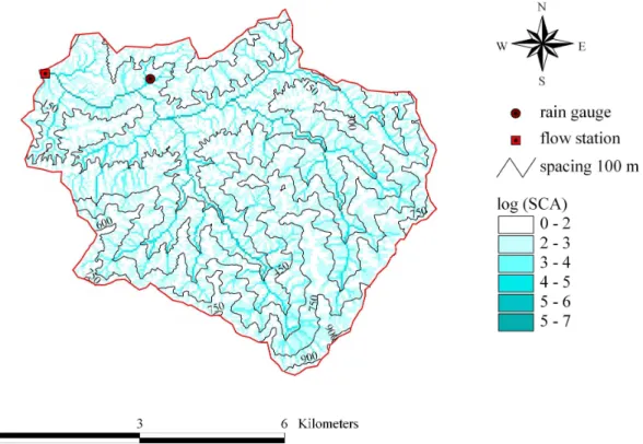
originates from Xiong-Kong Mt. (960 m a.s.l.) with its ele-vation from 180 to 960 m and an average slope of 41%. The topographic map and gauging stations are shown in Fig. 1. One hydrological station and only one rainfall station inside the watershed are maintained by the Water Resource Agency (www.wra.gov.tw).
The geologic setting in Heng-Chi watershed is mainly composed of sandstone and shale (Taiwan Central Geo-logical Survey, www.moeacgs.gov.tw). Strong weathering and erosion result in steep and deeply dissected landscape. Slopelands and low hills veneered by gravelly and sandy loam soils occupy∼90% of the watershed. Most rice fields and scattered farm houses are located in the gentle slopes at lower elevation while shrubbery, bamboo and primeval forest take up the slopes at higher elevation.
2.2 Extreme rain storms and flood events
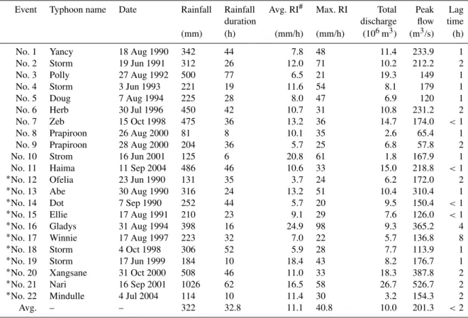
22 storm events are selected for this study (Table 1). Total rainfall among events ranges from 81 to 1026 mm with an av-erage rainfall intensity of 5.7–24.9 mm/h and the maximum rainfall intensity of 22–98 mm/h. Overall speaking, cumu-lative rainfalls are over 322 mm within 33 h. The total dis-charge ranges from 1.8 to 26.7 106m3positively correlated to total rainfall and rainfall duration. The peak flows range from 57.8 to 526.7 m3/s being positively correlated with to-tal rainfall, average rainfall intensity, and maximum rainfall intensity (Table 1).
Water discharge responds rapidly to rainfall with short time lag (generally less than 2 h). In most cases, the dis-charge surges approximately 100 times, from <2 m3/s to >200 m3/s within one hour. To investigate the model capa-bility for unknown events, the 22 events are separated equally into two subsets by total rainfall. That is, 11 events are for calibration and 11 events for validation. Each subset consists of similar range of total rainfall.
3 Methods
3.1 Three-layer structure and model formulation
The three-layer TOPMODEL contains eight processes: pre-cipitation, evapotranspiration, interception, infiltration, per-colation, surface flow, inter flow and base flow (see Fig. 2). Storage organization consists of three layers: 1) the upper layer, that is, the Root Zone, which has a fixed maximum water storage capacity, S1 max[L], and state variable of up-per layer storage, S1[L]; 2) the middle layer, which is the conventional Unsaturated Zone between ground surface and the ground water table, with soil moisture deficit,S2, [L] as
state variable; 3) the bottom layer, the Saturated Zone, below the ground water table withS3[L] as its storage. The three
Fig. 1.The Heng-Chi watershed. Stream network, elevation contour, specific contributing area (SCA) and hydrological stations are presented.
Fig. 2.Schematic diagram of the 3-layer TOPMODEL.
Once the rain falls, it is initially stored in the upper layer, where evapotranspiration occurs. The storage in the upper layer, S1, is controlled by rainfall and actual
evapotranspiration (Ea), which is determined by the ra-tio of S1 to S1 max and potential evapotranspiration (Ep).
TheEa[L/T] estimation is Ea=Ep
S1 S1 max
, if S1< S1 max (1a)
Table 1.The rainfall-runoff characteristics of the 22 events during 1990∼2004.
Event Typhoon name Date Rainfall Rainfall Avg. RI# Max. RI Total Peak Lag
duration discharge flow time
(mm) (h) (mm/h) (mm/h) (106m3) (m3/s) (h)
No. 1 Yancy 18 Aug 1990 342 44 7.8 48 11.4 233.9 1
No. 2 Storm 19 Jun 1991 312 26 12.0 71 10.2 212.2 2
No. 3 Polly 27 Aug 1992 500 77 6.5 21 19.3 149 1
No. 4 Storm 3 Jun 1993 221 19 11.6 54 8.1 179 1
No. 5 Doug 7 Aug 1994 225 28 8.0 47 6.9 120 1
No. 6 Herb 30 Jul 1996 450 42 10.7 31 10.8 231.2 2
No. 7 Zeb 15 Oct 1998 475 36 13.2 36 14.7 174.0 <1
No. 8 Prapiroon 26 Aug 2000 81 8 10.1 35 2.6 65.4 1
No. 9 Prapiroon 28 Aug 2000 204 36 5.7 25 6.8 57.8 2
No. 10 Strom 16 Jun 2001 125 6 20.8 61 1.8 167.9 1
No. 11 Haima 11 Sep 2004 486 46 10.6 33 15.0 218.8 <1
∗No. 12 Ofelia 23 Jun 1990 131 35 3.7 24 6.2 172.0 2
∗No. 13 Abe 30 Aug 1990 316 24 13.2 51 10.4 310.4 1
∗No. 14 Dot 7 Sep 1990 252 44 5.7 20 9.5 150.4 <1
∗No. 15 Ellie 17 Aug 1991 210 23 9.1 29 7.6 126.0 <1
∗No. 16 Gladys 31 Aug 1994 398 16 24.9 98 9.3 365.2 4
∗No. 17 Winnie 17 Aug 1997 223 32 7.0 22 5.7 136.8 8
∗No. 18 Storm 4 Oct 1998 306 52 5.9 28 7.7 113.9 1
∗No. 19 Storm 17 Jun 1999 184 10 18.4 43 8.2 176.7 1
∗No. 20 Xangsane 31 Oct 2000 508 46 11.0 33 18.3 387.8 2
∗No. 21 Nari 16 Sep 2001 1026 62 16.5 58 26.7 526.7 2
∗No. 22 Mindulle 4 Jul 2004 114 10 11.4 30 3.2 154.3 2
Avg. – – 322 32.8 11.1 40.8 10.0 201.3 <2
# RI indicates rainfall intensity;∗validation case.
The potential evapotranspiration can be determined by many methods (e.g. Penman, 1948; Monteith, 1965). Various factors such as temperature, wind speed, latitude, solar radia-tion, etc. are taken into account in certain methods. Although considering more factors in estimation might give better re-sults in some circumstances, yet, it implies additional mea-surements, extra cost, and higher level of model complexity. To reduce the complexity, we applied the simple empirical approximation by using temperature and latitude (Hamon, 1961). For event-based simulations, the potential evapotran-spiration estimation is neglected due to the much lower pro-portion between evapotranspiration to rainfall. OnceS1
ex-ceedsS1 maxdue to rainfall, the excess,qR[L], may have two paths. One is to infiltrate vertically down into the middle layer to increase soil moisture,qR,vand the other one is to form surface flow,qRhdepending on the middle layer is fully saturated or not. Once the middle layer is saturated, a vertical flux,P, percolates into the bottom layer from middle layer to elevateS3. In each time step,S2andS3are used to calculate,
respectively, theQi andQb. The routing calculations of the surface flow, inter flow and base flow are described below.
For surface flow, the flow path unit response function (Eq. 2) proposed by Liu et al., (2003) was applied. Note that Mannings’ equation and energy dissipation theory (Molnar
and Ramirez, 1998) were embedded to approach diffusion wave solution approximately.
The approximate solution is
U (t )= 1
σp2π·t3/t03exp "
−(t−t0)
2
2π t /t0 #
, (2)
and the outlet flow hydrograph can be represented as
QS(t )=
Z
A t Z
0
qRh(τ )·U (t−τ )dτ dA, (3)
whereU (t )[1/T] is the flow path unit response function;t0 [T] is the average travel time of the cell to outlet along flow path andσ[T] is the standard deviation of travel time. Both parameters, t0 andσ, are retrieved from DEMs (40-m
For inter flow,Qi[L3/T], we followed the formula in orig-inal TOPMODEL:
Qi =Qi0exp(−miS2), (4)
where [L3/T] is defined as a outflow parameter related to soil hydraulic properties and topography. In fact,Qi0is the
dis-charge when average soil moisture deficit equals zero. Ais the watershed area andmi is the recession coefficient of in-ter flow associated with soil characin-teristic. Paramein-ter,λ, the averaged soil-topographic index of the entire watershed, is defined as
λ= 1
A X
i
Ai ·ln ai
Titanβi, (5)
whereAi,ai,βi, andTi are cell area, specific contributing area, local slope, and local transmissivity, respectively, for inter flow associated with theicell.S2is the average of soil
moisture deficit for the entire watershed. The soil moisture deficit is the reduced moisture deficit per unit volume of soil from saturation (Walter et al., 2002),
S2=1− θ−θd
θs−θd
, (6)
whereθ is the average soil moisture content, θs is the sat-urated soil moisture content andθd is the air dry soil mois-ture content. Following the steady state assumption in TOP-MODEL, the soil moisture deficit for each grid is
S2,i =S2+
1 mi
λ−ln( ai Titanβi)
, (7)
whereS2,iis the soil moisture deficit forit hcell. The specific contributing area is derived from the infinite flow direction (Tarboton, 1997). Meanwhile the local slope gradient,βi is calculated by Zevenbergen and Throne’s method (1987). Ti is the local transmissivity for inter flow defined as the integral of hydraulic conductivity and soil depth.
The watershed average soil moisture deficit for each time step is updated by calculating the input and output in time steps,
S2,t =S2,t−1+(Qi,t−1−Qv,t/A)
Qv =P
i
qRv,i·Ai , (8)
whereQv is the total recharge to the middle layer in each time step. At timet=0, the initialS2is estimated by
S2,t=0= −
1 mi ln(
0.2·Qobs,t=0 Qi0
), (9)
whereQobs,t=0is the observed discharge at timet=0. Note
that the proportion of inter flow over total stream discharge in the initial condition is assigned to be 0.2. Once the initial catchment average soil moisture deficit is decided, the spa-tial pattern is implanted by Eq. (7). Some other methods had been proposed to replace Eq. (7) to mimic the spatial pattern,
such as Troch et al. (1993) and Barling et al. (1994). Since we focus on the applicability of this TOPMODEL, the origi-nal implement is applied.
For base flow calculation, we applied the exponential re-cession curve function (Lamb and Beven, 1997),
Qb=Qb0exp(−mb·S3), (10)
where mb is the recession coefficient and Qb0 is the
dis-charge when the base flow storage deficit equals zero. Note thatQi0andQb0are different owing to different
transmis-sivity, but share the sameKandD. Similar to inter flow, the base flow deficit is also updated in each step by following water balance,
S3,t−1=S3,t−1+(Qb,t−1−Qp,t/A)
Qp =P
i
Pi ·Ai , (11)
whereQpis the total recharge from the middle layer to the saturated zone. Note that only when the cell in the middle layer is saturated, the percolation,P[L/T], will recharge the bottom layer. Besides, the initial bottom layer storage is rep-resented as
S3,t=0= −
1 mbln(
0.8·Qobs,t=0 Qb0
). (12)
Thus the three flows can be simulated step by step when hourly rainfall inputted.
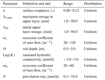
Collectively, eight global parameters in functions afore-mentioned are essential to route the model: maximum stor-age (S1 max) in the upper layer, initial value of (S10), surface
roughness (n), soil characteristic parameter (mi), saturated hydraulic conductivity (K), soil depth (D), base flow reces-sion coefficient (mb), and percolation rate (P). The main model outputs for each time step include the spatial pattern of soil moisture for the entire watershed and stream discharge at outlet, which composes of simulated surface flow, inter flow and base flow.
TOPMODEL is a spatially distributed model. Many pre-vious studies utilized the capacity and applied the land cover map, vegetation cover and soil map to represent the parameter distribution in space. Those kind of dis-tributed maps introduce their ordinary-scale (classification) information; however, converting these categories into pa-rameter values (interval- or ratio-scale) is highly uncertain (Wang et al., 2006) and case dependent. It may also raise the fog of equifinality as well (Beven and Freer, 2001). More-over, some model parameters only represent conceptual en-tities, which may not be measured directly (Refsgaard et al., 2006). For example, soil transmissivity in TOPMODEL has been proven that it is a scale parameter with grid size (Fran-chini et al., 1996).
3.2 Parameter calibration and performance measure Parameter calibration is essential because of the limita-tions of model structure and data availability of parameters, namely, initial conditions and boundary conditions. During calibration various measures were proposed to quantify the performance of hydrological simulation. Those measures de-pend on different purposes such as hydrograph shape, peak flow, peak time, discharge volume or even low flow (e.g. Krause et al., 2005). Different measures, apparently, extract different satisfactory combinations for their own aspect.
Here, we combine the overall root mean square error (ORMSE) and average root mean square error of peak flow (ARMSE) with equal weights (Madsen, 2000) to serve as our performance measure (CRMSE). The following formulas de-fine ORMSE, ARMSE, and CRMSE:
ORMSE= N P
i=1 w2i
Qs,i−Qo,i2 N
P
i=1 wi2
1/2
, (13)
ARMSE= 1
Mp Mp
X
j=1 nj P
i=1
wi2Qs,i−Qo,i2 nj
P
i=1 w2i
1/2
, (14)
CRMSE=1
2ORMSE+ 1
2ARMSE. (15)
In Eqs. (13)–(15),Qo,iis the observed discharge at timei, Qs,iis the simulated discharge,Nis the total time step in the individual events,Mpis the number of peak flow events,nj is the number of time steps in peak flow periods andwi is the weighting function. Peak flow periods are defined as periods when the observed discharge is >100 m3/s. This measure concerns both hydrograph shape and peak flow that are most important for flood warning.
To present differences between simulation and observa-tion, we further provide 5 indicators, namely, EC, EClog,
EQV, EQP, and EQT. All five indicators are often used in evaluating hydrograph simulation. The efficiency coefficient (EC) proposed by Nash and Sutcliffe (1970) can quantify the overall deviation between simulated and observed hydro-graphs. The highest value of EC is 1.0. To better quantify the similarity in low flow condition, EClog, the logarithmic
Nash-Sutcliffe efficient (e.g. G¨untner et al., 1999; De Smedt et al., 2000), is applied due to its ability to reproduce time evolution of low flow. The other three indicators: the error of total discharge volume (EQV) is defined as the ratio of sim-ulated total flow over observed total flow; the error of peak flow (EQP) is defined as the ratio of simulated peak flow over observed peak flow, and the error of time to peak (EQT) is de-fined as the deviation between times of simulated peak and
observed peak. Through the five indicators the performance of simulations can be evaluated comprehensively.
To extract the global best-fitted combination, 20 000 pa-rameter sets are generated by random uniform-distribution generator (Table 2). The uniform distribution is gener-ally adapted for generating parameters when information about the parameter population is insufficient. Based on the 20 000 parameter combinations, 20 000 predictions and correspondent CRMSE values for each event are acquired. Among the 20 000 predictions we obtain the best-fitted com-bination (with lowest CRMSE value) for each event individ-ually. However, the best-fitted combination may not be the best for the other events; therefore all CRMSE values are summed to evaluate the overall performance of the respective parameter set. This overall performance serves as a criterion to single out the global best-fitted combination.
4 Results and discussion
4.1 Best-fitted simulation and calibration
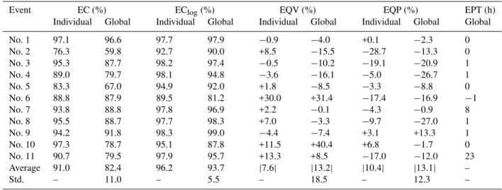
Simulations derived from the global best-fitted and the event best-fitted combination are compared by using the 5 indica-tors mentioned above (Table 3). For individual event, best-fitted EC varies from 83.3∼97.3% with an average EC of 91.0%. EClogvalues range from 89.5 to 98.3% with an
av-erage of 96.2%. The means of absolute value of EQV and EQP are 7.6% and 10.4%, respectively. Generally speaking, the near-perfect simulation can be derived from specific com-bination. However, those different combinations may not be the same and cannot be used for validation and practical ap-plications.
Contrast to individual results, those simulations based on the global best-fitted combination:n=0.13,S1 max=14.9 mm, S10=15.9 mm, mi=80.2, D=3.1 m, K=130 mm/h, mb=22.1, P=4.6 mm/h are also presented. EC values of simulations de-rived from global best-fitted set vary from 59.8 to 96.6% with an average of 82.4%, which is lower than independent simu-lations (Table 3). The global best-fitted set gives EClogvalues
from 81.2 to 99.0% with an average of 93.7%. Meanwhile, the means of absolute value of EQV and EQP are 13.2% and 13.1%, respectively. The standard deviations of EC, EClog,
Table 2. The description, sampling range, and distribution of the 8 input parameters.
Parameter Definition and unit Range Distribution
n surface roughness, [-] 0.08∼0.22 Uniform
S1 max maximum storage in
upper layer, [mm] 1.0∼50.0 Uniform
S10 initial upper
layer storage, [mm] 1.0∼50.0 Uniform
mi recession coefficient
of inter flow, [m−1] 20∼120 Uniform
D soil depth, [m] 0.5∼5.0 Uniform
Log(K) saturated hydraulic
conductivity, [mm/h] −3.0∼3.0 Uniform
mb recession coefficient 20∼60 Uniform
of base flow, [m−1]
P percolation rate, [mm/h] 0.1∼10.0 Uniform
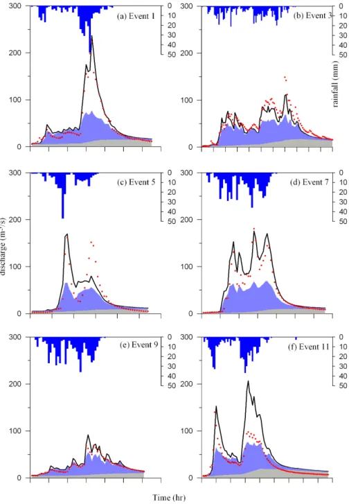
hydrograph, respond rapidly. Surface flow dominates partic-ularly under torrential and concentrated rainfall conditions, such as event 1, 7, and 11 (Fig. 3a, d, and f), whereas, the inter flow dominates when the rainfall is relative small and gentle, such as Events 3 and 9 (Fig. 3b and e). Obviously, rainfall characteristics may regulate the relative contribution of surface flow and inter flow in model. Third, the base flow, which occupies a relatively small portion of total discharge, always shows slow response.
Honestly, although we have good performances in using the 3-layer TOPMODEL, geochemical tracers or other ad-vanced techniques are still needed to validate the three flow components. Note that many hydrological models based on different runoff generation mechanism or different storages can also give equal performances (Beven and Freer, 2001; Steenhuis et al., 1999) after calibration, so called equifinality. Apparently, it is insufficient that only using stream discharge to evaluate runoff generation mechanism and storages. In our case, nevertheless, the calibrated saturated hydraulic con-ductivity (130 mm/h) is higher than the maximum rainfall in-tensity. Such higherK might indirectly support saturation excess runoff mechanism in subtropical mountainous water-sheds as indicated by Walter et al. (2003). Meanwhile, no Hortonian flow was observed in the field during our typhoon monitoring in 2007. In addition, our preliminary result of geochemical tracers (unpublished data) suggests three com-ponents in stream discharge. Those indirect evidences sup-port the potential of 3-layer structure for this kind of water-shed.
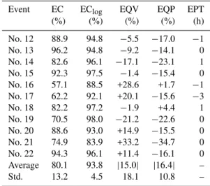
4.2 Validation and inter-comparison among events After calibration, the global best-fitted combination is ap-plied onto validation events and the simulations are presented in Table 4. The EC values vary from 57.1∼96.2% with an av-erage of 80.1%. The EClogvalues range from 88.5∼98.0%
with an average of 93.8%. Meanwhile, the means of absolute values of EQV and EQP are 15.0 and 16.4%, respectively, with ranges of−21.2–+33.2% and−34.7–+4.4%. And the standard deviations of EC, EClog, EQV, and EQP are 13.2,
4.5, 18.1, and 10.8, respectively.
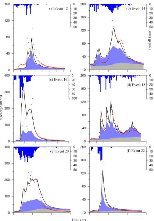
For validation events, 6 examples of simulated hydro-graphs are shown in Fig. 4. The features of the simulated hy-drographs resemble those presented in Fig. 3. Since selected events cover a wide range of total rainfall, we compare the four indicators against the total rainfall (Fig. 5). Most vali-dation events fall within±1 standard deviation of respective indicator indicating that the overall performances of valida-tion events are similar to those of calibravalida-tion events. In addi-tion, this figure also shows the performances are irrelative to total rainfall. Thus we have confidence to apply our model for various rain storms for management.
Fig. 3. The 6 examples among 11 calibration events for simulated and observed hydrographs with corresponded hyetographs. The red dot stands for observation; black curve represents simulation. Gray and blue gray zones indicate, respectively, the base and inter flows.
4.3 Parameter sensitivity in hydrograph simulation Though the model applicability is presented, the parameter behaviors and it effects on model efficiency are still not clear. Computation efficiency in calibration can be significantly im-proved if we know which parameters are most sensitive to model simulations (Sieber et. al., 2005; Tang et al., 2007).
Fig. 4. The 6 examples among 11 validation events for simulated and observed hydrographs with corresponded hyetographs. The red dot stands for observation; black curve represents simulation. Gray and blue gray zones indicate, respectively, the base and inter flows.
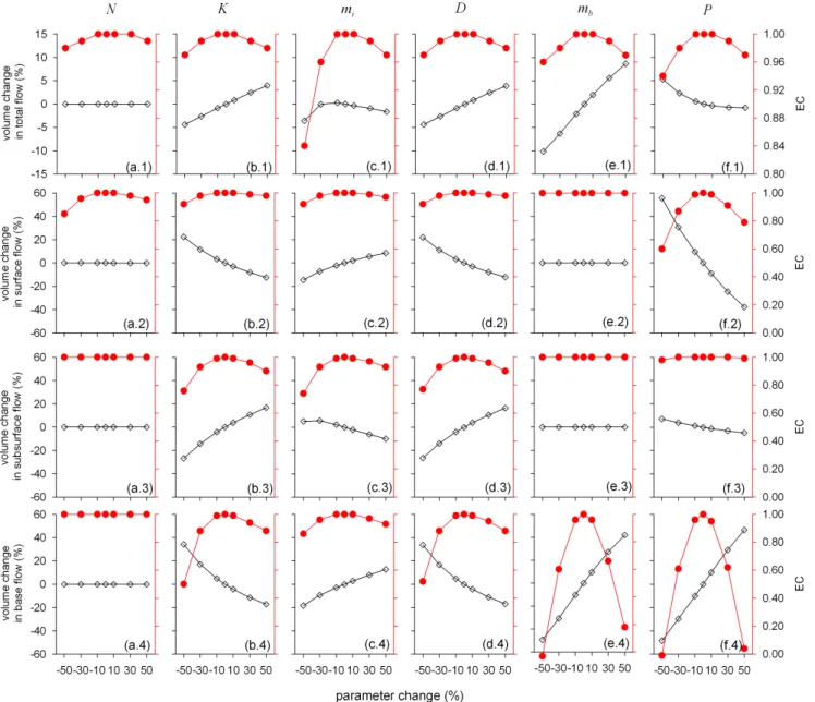
In Fig. 6, the 6 uppermost panels are for total discharge, we can see EC value changes as parameter changes (Fig. 6.a1– f1). ParameterP andmi are the most effective on shape likelihood in terms of integrated hydrograph. However, the base flow is the most responsive component to changes inP andmband the subsurface flow is responsive to changes in K,mi andD. Surface roughness (n) does not alter the dis-charge volume and only affect the hydrograph shape in sur-face flow (Fig. 6a.1–4). This parameter determines sursur-face
flow’s traveling time (or surface flow velocity). The smaller n values cause faster response and consequently sharper hy-drograph. Each parameter has its own effects on EC and/or total discharge.
Table 3.Simulation results of the 11 calibration events by individual and global best-fitted parameter set.
Event EC (%) EClog(%) EQV (%) EQP (%) EPT (h)
Individual Global Individual Global Individual Global Individual Global Global
No. 1 97.1 96.6 97.7 97.9 −0.9 −4.0 +0.1 −2.3 0
No. 2 76.3 59.8 92.7 90.0 +8.5 −15.5 −28.7 −13.3 0
No. 3 95.3 87.7 98.2 97.4 −0.5 −10.2 −19.1 −20.9 1
No. 4 89.0 79.7 98.1 94.8 −3.6 −16.1 −5.0 −26.7 1
No. 5 83.3 67.0 94.9 92.0 +1.8 −8.5 −3.3 −8.8 0
No. 6 88.8 87.9 89.5 81.2 +30.0 +31.4 −17.4 −16.9 −1
No. 7 93.8 88.8 97.8 96.9 +2.2 −0.1 −4.3 −0.9 8
No. 8 95.5 88.7 97.7 98.3 +7.0 −3.3 −9.7 −27.0 1
No. 9 94.2 91.8 98.3 99.0 −4.4 −7.4 +3.1 +13.3 1
No. 10 97.3 78.7 95.1 87.8 +11.5 +40.4 +6.8 −1.7 0
No. 11 90.7 79.5 97.9 95.7 +13.3 +8.5 −17.0 −12.0 23
Average 91.0 82.4 96.2 93.7 |7.6| |13.2| |10.4| |13.1| –
Std. – 11.0 – 5.5 – 18.5 – 12.3 –
| |stands for the absolute value.
Fig. 5. Scatter plots of performance indicators against total rainfall. Dash lines and gray zones are the means and standard deviations, respectively, derived from calibration events. Squares and crosses mark, respectively, the calibration and validation events.
changes corresponds to 50% changes inmb. However, its effect is mainly caused by changes in base flow, which com-posed of∼30% of total discharge, thus its influence on total discharge is compromised though over 40% changes in base flow can be induced. Parametermbcontrols the resident time in bottom layer and therefore has a significant effect on the amount of base flow but no interactive effect on surface or inter flows (Fig. 6e.2–4). In general,mi reflects mainly the
velocity of inter flow. Highermi may induce a faster change in soil moisture deficit, thus, may cause a larger saturated area to enhance the surface and base flows (Fig. 6c.2) and diminish the inter flow significantly (Fig. 6c.3).
Fig. 6.The percent change in discharge and EC response against parameter change. The x-axis shows percent change in individual parameter based on the global best-fitted combination. Left y-axis corresponded to empty diamonds represent percent changes in discharge. Right y-axis corresponded to red circles stands for the percent changes in EC. Note that y-axis is in different range.
response. HigherKandDallow the water infiltrate to mid-dle layer and reduce the surface and base flow (Fig. 6b and d). Addition tomb,K, andD, parameterP is also effective on total discharge (Fig. 6 f.1–4). AsP increases, the surface flow volume decreases significantly. HigherP diminishes the surface and inter flow and increase the base flow.
Our results of sensitivity analysis may guide the prior-ity in field measurements and shed lights on process inter-actions inside models to strengthen our understanding on model structure and re-examine the rationality of model hy-pothesis.
4.4 Confidence interval
Table 4.Simulation results of validation events by the global best-fitted parameter set.
Event EC EClog EQV EQP EPT
(%) (%) (%) (%) (h)
No. 12 88.9 94.8 −5.5 −17.0 −1
No. 13 96.2 94.8 −9.2 −14.1 0
No. 14 82.6 96.1 −17.1 −23.1 1
No. 15 92.3 97.5 −1.4 −15.4 0
No. 16 57.1 88.5 +28.6 +1.7 −1
No. 17 62.2 92.1 +20.1 −15.6 −3
No. 18 82.2 97.2 −1.9 +4.4 1
No. 19 70.5 98.0 −21.2 −22.6 0
No. 20 88.6 93.0 +14.9 −15.5 0
No. 21 74.9 83.9 +33.2 −34.7 0
No. 22 94.3 96.1 +11.4 −16.1 0
Average 80.1 93.8 |15.0| |16.4| –
Std. 13.2 4.5 18.1 10.8 –
Table 5. Empirically-based confident interval and success rate in validation.
Discharge Lower Median Upper Success rate
category limit limit in validation
(m3/s)
<4.8 0.60 1.30 3.54 0.93
4.8–7.2 0.72 1.08 2.01 0.78
7.2–10.8 0.55 0.89 1.70 0.88
10.8–15.6 0.66 1.00 1.68 0.76
15.6–23.9 0.41 0.94 1.45 0.92
23.9–33.6 0.47 0.90 1.65 0.97
33.6–44.7 0.52 0.88 1.58 0.92
44.7–74.5 0.45 0.92 1.52 0.88
74.5–124.7 0.40 0.90 1.40 0.94
>124.7 0.40 0.94 1.53 0.98
Firstly, the simulated discharges in calibration are divided into 10 categories by occurrence. Secondly, we calculate the median, 5% and 95% limits ofQobs/Qsimratios in each
cat-egory. The two limits embrace 90% of simulations during calibration. Thirdly, we calculate the success rate in vali-dation. Furthermore, by multiplying the simulation by the two limits we generate upper and lower boundaries of confi-dence for management use. Conceptually, it is without value if the confidence interval is too wide. On the other hand, we may obtain a narrow one in certain circumstance when data length is insufficiently long; it will be risky to apply the narrow one since it might give low success rate in vali-dation. This confidence interval is empirically-based, thus, data length is crucial.
Fig. 7.Scatter plot of theQobs/Qsimagainst Qsim. Red dots stand for validation events. Black lines are the median and the gray zones are 90% confidence interval derived from all calibration events.
Here we list the medians, lower limits, upper limits, and success rate in validation for different discharge categories in Table 5. The medians of the 10 categories are close to 1.0 (except category 1 with underestimation) and the width of 90% confidence interval (upper-lower) ranges from 0.48∼1.56 (not shown). Meanwhile, mean success rate is 89.9±0.1. Such promising results indicate that our model simulates well over wide water discharges. We also present Qobs/Qsim ratio against Qsim (Fig. 7) to reveal how the
empirically-based confidence interval envelope observed dis-charges in validation events. Our newly proposed confidence interval (Table 5) may serve as a crucial reference for future hydrograph predictions. The upper limit is suggested prefer-ably for flood risk assessment and the lower limit preferprefer-ably for drought assessment.
5 Conclusions
This study presents the capability of a 3-layer TOPMODEL in simulating flood hydrograph induced by wide ranges of torrential rainfalls in a subtropical mountainous watershed in Taiwan. The global best-fitted combination gives an average performance of 82.4% in EC and 93.7% in EClogfor 11
cal-ibration events and 80.1% in EC and 93.8% in EClogfor
the hydrograph compositions deepening our understanding on real rainfall-runoff response and approaching better model structure. On the other hand, the influence of storm charac-teristics on runoff generation should be explored to improve model performances.
Acknowledgements. This research is funded by the National Science Council of Taiwan, under the project NSC 95-2116-M-001-001. The authors are also grateful to Water Resources Agency and Chun-Chiang Lin in Lan Yang Institute of Technology for providing hydrological records and computation facility. We also appreciate A. Gelfan and two anonymous reviewers for their useful comments.
Edited by: A. Gelfan
References
Barling, R. D., Moore, I. D., and Grayson, R. B.: A quasi-dynamic wetness index for characterizing the spatial distribution of zones of surface saturation and soil water content, Water Resour. Res., 30, 1029–1044, 1994.
Beven, K. J.: TOPMODEL: a critique, Hydrol. Process., 11(9), 1069–1086, 1997.
Beven, K. J.: Parameter Estimation and Predictive Uncertainty, in: Rainfall-Runoff Modelling, edited by: Beven, K. J., The Primer, WILEY, New York, 217–253, 2001.
Beven, K. J. and Freer, J.: Equifinality, data assimilation, and uncer-tainty estimation in mechanistic modeling of complex environ-mental systems using the GLUE methodology, J. Hydrol., 249, 11–29, 2001
Campling, P., Gobin, A., Beven, K., and Feyen, J.: Rainfall-runoff modeling of a humid tropical catchment: the TOPMODEL ap-proach, Hydrol. Process., 16(2), 231–253, 2002.
Candela, A., Noto, L. V., and Aronica, G.: Influence of surface roughness in hydrological response of semiarid catchments, J. Hydrol., 313, 119–131, 2005.
Casadei, M., Dietrich, W. E., and Miller, N. L.: Testing a model for predicting the timing and location of shallow landslide initiation in soil mantled landscapes, Earth Surf. Processes, 28(9), 925– 950, 2003.
De Smedt, F., Liu, Y. B., and Gebremeskel, S.: Hydrological mod-eling on a catchment scale using GIS and remote sensed land use information, in: Risk Analysis II, edited by: Brebbia, C. A., WTI press, Southampton, Boston, 295–304, 2000.
Franchini, M., Wendling, J., Obled, C., and Todini, E.: Physical in-terpretation and sensitivity analysis of the TOPMODEL, J. Hy-drol., 175, 293–338, 1996.
G¨unter, A., Uhlenbrook, S., Seibert, J., and Leibundgut, C.: Multi-criterial validation of TOPMODEL in a mountainous catchment, Hydrol. Process., 13, 1603–1620, 1999.
Hamon, W. R.: Estimating potential evapotranspiration: Proceed-ings of the American Society of Civil Engineers, J. Hydr. Eng. Div.-ASCE, 87(HY3), 107–120, 1961.
Hornberger, G. M., Scanlon, T. M., and Raffensperger, J. P.: Mod-elling transport of dissolved silica in a forested headwater catch-ment: the effect of hydrological and chemical time scales on
hys-teresis in the concentration-discharge relationship, Hydrol. Pro-cess., 15(10), 2029–2038, 2001.
Huang, J. C., Kao, S. J., Hsu, M. L., and Lin, J. C.: Stochastic pro-cedure to extract and to integrate landslide susceptibility maps: an example of mountainous watershed in Taiwan, Nat. Hazards Earth Syst. Sci., 6, 803–815, 2006,
http://www.nat-hazards-earth-syst-sci.net/6/803/2006/.
Huang, J. C. and Kao, S. J.: Typhoon-induced storm hydro-graph simulations versus parameter sensitivity in a 3-layer TOP-MODEL: A case study in a subtropical mountainous watershed, 4th AOGS Annual Meeting, Bangkok, Thailand, 2007.
Krause, P., Boyle, D. P., and B¨ase, F.: Comparison of different ef-ficiency criteria for hydrological model assessment, Advances in Geosciences, 5, 89–97, 2005.
Lamb, R. and Beven, K.: Using interactive recession curve analysis to specify a general catchment storage model, Hydrol. Earth Syst. Sci., 1, 101–113, 1997,
http://www.hydrol-earth-syst-sci.net/1/101/1997/.
Lamb, R., Beven, K., and Myrabø, S.: A generalized topographic-soils hydrological index, in: Landform Monitoring, Modeling and Analysis, edited by: Lans, S. N., Richards, K. S., Chandler, J. H., John Wiley, Chichester, 263–278, 1998.
Li, M. H., Yang, M. J., Soong, R., and Huang, H. L.: Simulating typhoon floods with gauge data and mesoscale modeled rainfall in a mountainous watershed, J. Hydrometeorol., 6(3), 306–323, 2005.
Liu, Y. B., Gebremeskel, S., De Smedt, F., Hoffman, L., and Pfister, L.: A diffusive approach for flow routing in GIS based flood modeling, J. Hydrol., 283, 91–106, 2003.
Madsen, H.: Automatic calibration of a conceptual rainfall-runoff model using multiple objectives, J. Hydrol., 235 276–288, 2000.
Molnar, P. and Ramirez, J. A.: Energy dissipation theories and opti-mal channel characteristics of river network, Water Resour. Res., 34(7), 1809–1818, 1998.
Monteith, J. L.: Evaporation and environment, Sym. Soc. Exp. Biol., 19, 205–234, 1965.
Nash, J. E. and Sutcliffe, J. V.: River flow forecasting through con-ceptual models 1. A discussion of principles, J. Hydrol., 10, 282– 290, 1970.
Pebesma, E. J., Switzer, P., and Loague, K.: Error
analy-sis for the evaluation of model performance: rainfall-runoff event summary variables, Hydrol. Process., 21, 3009–3024, doi:10.1002/hyp.6529, 2007.
Penman, H. L.: Natural evaporation from open water, bare soil, and grass, P. Roy. Soc. Lond. A, 193, 120–195, 1948.
Reaney, S. M., Bracken, L. J., and Kirkby, M. J.: Use of the con-nectivity of runoff model (CRUM) to investigate the influence of storm characteristics on runoff generation and connectivity in semi-arid areas, Hydrol. Process., 21, 894–906, 2007.
Refsgaard, J.C., van der Sluijs, J. P., Brown, J., and van der Keur, P.: A framework for dealing with uncertainty due to model structure error, Adv. Water Resour., 29, 1586–1597, 2006.
Scanlon, T. M., Raffensperger, J. P., and Hornberger, G. M.: Shal-low subsurface storm fShal-low in a forested headwater catchment: Observations and modeling using a modified TOPMODEL, Wa-ter Resour. Res., 36(9), 2575–2586, 2000.
216–235, 2005.
Steenhuis, T. S., Parlange, J. Y., Sanford, W. E., Heilig, A., Stag-nitti, F., and Water, M. F.: Can we distinguish Richard’s and Boussinesq’s equations for hillslopes? The Coweeta experiment revisited, Water Resour. Res., 35(2), 589–293, 1999.
Sui, C. H., Huang, C. Y., Tsai, Y. B., Chen, C. S., Lin, P. L., Shieh, S. L., Li, M. H., Liou, Y. A., Wang, T. C. C., Wu, R. S., Liu, G. R., and Chu, Y. H.: Meteorology-hydrology study targets Ty-phoon Nari and Taipei Flood, Eos. T, Am. Geophys. Un., 83(24), 265–270, 2002.
Tang, Y., Reed, P., Wagener, T., and van Werkhoven, K.: Comparing sensitivity analysis methods to advance lumped watershed model identification and evaluation, Hydrol. Earth Syst. Sci., 11, 793— -817, 2007,
http://www.hydrol-earth-syst-sci.net/11/793/2007/.
Tarboton, D. G.: A new method for the determination of flow di-rections and con tributing areas in grid digital elevation models, Water Resour. Res., 33(2), 309–319, 1997.
Troch, P. A. and De Troch, F. P.: Effective water Table depth to de-scribe initial conditions prior to storm rainfall in humid regions, Water Resour. Res., 29(2), 427–434, 1993.
Walter, M. T., Steenhuis, T. S., Mehta, V. K., Thongs, D., Zion, M., and Schneiderman, E.: Refined conceptualization of TOP-MODEL for shallow subsurface flows, Hydrol. Process., 16, 2041–2046, 2002.
Walter, M. T., Mehta, V. K., Marrone, A. M., Boll, J., Gerard-Marchant, P., Steenhuis, T. S., and Walter, M. F.: Simple Esti-mation of Prevalence of Hortonian Flow in New York City Wa-tersheds, J. Hydrol. Eng., 8(4): 214–218, 2003.
Wang, Y. C., Han, D., Yu, P. S., and Cluckie, I. D.: Comparative modeling of two catchments in Taiwan and England, Hydrol. Process., 20(20), 4335–4349, 2006.
Wu, L., Wang, B., and Geng, S.: Growing typhoon
influ-ence on east Asia, Geophys. Res. Lett., 32(18), L18703, doi:10.1029/2005GL022937, 2005.