www.atmos-chem-phys.net/16/15629/2016/ doi:10.5194/acp-16-15629-2016
© Author(s) 2016. CC Attribution 3.0 License.
Insights into the deterministic skill of air quality ensembles
from the analysis of AQMEII data
Ioannis Kioutsioukis1,2, Ulas Im3, Efisio Solazzo2, Roberto Bianconi4, Alba Badia5, Alessandra Balzarini6, Rocío Baró12, Roberto Bellasio4, Dominik Brunner7, Charles Chemel8, Gabriele Curci9,10,
Hugo Denier van der Gon11, Johannes Flemming13, Renate Forkel14, Lea Giordano7, Pedro Jiménez-Guerrero12, Marcus Hirtl15, Oriol Jorba5, Astrid Manders-Groot11, Lucy Neal16, Juan L. Pérez17, Guidio Pirovano6,
Roberto San Jose16, Nicholas Savage15, Wolfram Schroder18, Ranjeet S. Sokhi8, Dimiter Syrakov19, Paolo Tuccella9,10, Johannes Werhahn14, Ralf Wolke18, Christian Hogrefe20, and Stefano Galmarini2
1University of Patras, Department of Physics, University Campus 26504 Rio, Patras, Greece
2European Commission, Joint Research Centre, Directorate for Energy, Transport and Climate, Air and Climate Unit,
Ispra (VA), Italy
3Aarhus University, Department of Environmental Science, Roskilde, Denmark 4Enviroware srl, Concorezzo (MB), Italy
5Earth Sciences Department, Barcelona Supercomputing Center (BSC-CNS), Barcelona, Spain 6Ricerca sul Sistema Energetico (RSE) SpA, Milan, Italy
7Laboratory for Air Pollution and Environmental Technology, Empa, Dubendorf, Switzerland
8Centre for Atmospheric & Instrumentation Research, University of Hertfordshire, College Lane, Hatfield, AL10 9AB, UK 9Department of Physical and Chemical Sciences, University of L’Aquila, L’Aquila, Italy
10Center of Excellence for the forecast of Severe Weather (CETEMPS), University of L’Aquila, L’Aquila, Italy 11Netherlands Organization for Applied Scientific Research (TNO), Utrecht, the Netherlands
12University of Murcia, Department of Physics, Physics of the Earth, Campus de Espinardo, Ed. CIOyN, 30100 Murcia, Spain 13ECMWF, Shinfield Park, Reading, RG2 9AX, UK
14Karlsruher Institut für Technologie (KIT), IMK-IFU, Kreuzeckbahnstr. 19, 82467 Garmisch-Partenkirchen, Germany 15Zentralanstalt für Meteorologie und Geodynamik, ZAMG, 1190 Vienna, Austria
16Met Office, FitzRoy Road, Exeter, EX1 3PB, UK
17Environmental Software and Modelling Group, Computer Science School – Technical University of Madrid, Campus de
Montegancedo – Boadilla del Monte, 28660 Madrid, Spain
18Leibniz Institute for Tropospheric Research, Permoserstr. 15, 04318 Leipzig, Germany
19National Institute of Meteorology and Hydrology, Bulgarian Academy of Sciences, 66 Tzarigradsko shaussee Blvd.,
1784 Sofia, Bulgaria
20Atmospheric Modelling and Analysis Division, Environmental Protection Agency, Research, Triangle Park, USA
Correspondence to:Stefano Galmarini ([email protected])
Abstract. Simulations from chemical weather models are subject to uncertainties in the input data (e.g. emission ventory, initial and boundary conditions) as well as those in-trinsic to the model (e.g. physical parameterization, chemical mechanism). Multi-model ensembles can improve the fore-cast skill, provided that certain mathematical conditions are fulfilled. In this work, four ensemble methods were applied to two different datasets, and their performance was com-pared for ozone (O3), nitrogen dioxide (NO2) and
particu-late matter (PM10). Apart from the unconditional ensemble
average, the approach behind the other three methods re-lies on adding optimum weights to members or constrain-ing the ensemble to those members that meet certain condi-tions in time or frequency domain. The two different datasets were created for the first and second phase of the Air Qual-ity Model Evaluation International Initiative (AQMEII). The methods are evaluated against ground level observations col-lected from the EMEP (European Monitoring and Evaluation Programme) and AirBase databases. The goal of the study is to quantify to what extent we can extract predictable signals from an ensemble with superior skill over the single models and the ensemble mean. Verification statistics show that the deterministic models simulate better O3than NO2and PM10,
linked to different levels of complexity in the represented processes. The unconditional ensemble mean achieves higher skill compared to each station’s best deterministic model at no more than 60 % of the sites, indicating a combination of members with unbalanced skill difference and error depen-dence for the rest. The promotion of the right amount of ac-curacy and diversity within the ensemble results in an aver-age additional skill of up to 31 % compared to using the full ensemble in an unconditional way. The skill improvements were higher for O3and lower for PM10, associated with the
extent of potential changes in the joint distribution of accu-racy and diversity in the ensembles. The skill enhancement was superior using the weighting scheme, but the training period required to acquire representative weights was longer compared to the sub-selecting schemes. Further development of the method is discussed in the conclusion.
1 Introduction
Uncertainties in atmospheric models, such as the chemical weather models, whether due to the input data or the model itself, limit the predictive skill. The incorporation of data as-similation techniques and the continued effort in understand-ing the physical, chemical and dynamical processes result in better forecasts (Zhang et al., 2012). In addition, ensemble methods provide an extra channel for forecast improvement and uncertainty quantification. The benefits from ensemble averaging arise from filtering out the components of the fore-cast with uncorrelated errors (Kalnay, 2003).
The European Centre for Medium-Range Weather Fore-cast (ECMWF) reports an increase in foreFore-cast skill of 1 day per decade for meteorological variables, evaluated on the geopotential height anomaly (Simmons, 2011). The air qual-ity modelling and monitoring has a shorter history that does not allow a similar adequate estimation of such trends for the numerous species being modelled. Moreover, the skill changes dramatically from species to species and is strongly connected to the availability of accurate emission data. Re-sults for ozone suggest that medium-range forecasts can be performed with a quality similar to the geopotential height anomaly forecasts (Eskes et al., 2002). Aside from the con-tinuous increase in skill due to the improved scientific un-derstanding, harmonized emission inventories, more accu-rate and denser observations, as well as ensemble averag-ing, an extra gain of similar magnitude can be achieved for ensemble-based deterministic modelling using conditional averaging (e.g. Galmarini et al., 2013; Mallet et al., 2009; Solazzo et al., 2013).
Ideally, for continuous and unbiased variables, the multi-model ensemble mean outscores the skill of the deterministic models provided that the members have similar skill and in-dependent errors (Potempski and Galmarini, 2009; Weigel et al., 2010). Practically, the multi-model ensemble mean usu-ally outscores the skill of the deterministic models if the evaluation is performed over multiple observation sites and times. This occurs because over a network of stations, there are some where the essential conditions (e.g. the skill dif-ference between the models is not too large) for the ensem-ble members are fulfilled, favouring the ensemensem-ble mean; for the remaining stations, where the conditions are not fulfilled, local verification identifies the best model, but generally no single model is the best at all sites. Hence, although the skill of the numerical models varies in space (latitude, longitude, altitude) and time (e.g. hour of the day, month, season), the ensemble mean is usually the most accurate spatio-temporal representation.
The majority of those ensemble studies focus on O3, and only
recently the studies also involve particulate matter (Djalalova et al., 2010; Monteiro et al., 2013).
In this work, we apply and intercompare both approaches (weighting and sub-selecting) using the Air Quality Model Evaluation International Initiative (AQMEII) datasets from phase I and phase II. The ensemble approaches are evalu-ated against ground level observations from the EMEP (Eu-ropean Monitoring and Evaluation Programme) and Air-Base databases, focusing on the pollutants O3, NO2 and
PM10 that exhibit different levels of forecast skill. The
dif-ferences between the multi-model ensembles of phase I (hereafter AQMEII-I) and phase II (hereafter AQMEII-II) originate from many sources, related to both the input data and the models: (a) the simulated years are different (2006 vs. 2010); therefore, the meteorological conditions are different. (b) Emission methodologies have changed, (c) boundary conditions are very different, (d) the composi-tion of the ensembles is different, (e) the models in AQMEII-II use online coupling between meteorology and chemistry, and (f) the models may have been updated with new science processes apart from feedback processes. The uncertainties arising from observational errors are not taken into consider-ation.
In spite of these differences we consider the analysis of the two sets of ensembles revealing. In detail, the objectives of the paper are (a) to interpret the skill of the unconditional multi-model mean within AQMEII-I and AQMEII-II, (b) to calculate the maximum expectations in the skill of alternative ensemble estimators and (c) to evaluate the operational im-plementation of the approaches using cross-validation. The originality of the study includes (a) the comparison of sev-eral ensemble methods on pollutants of different skill using different datasets, (b) the introduction of an approach based on high-dimension spectral optimization, and (c) the intro-duction of innovative charts for the interpretation of the error of the unconditional ensemble mean with respect to indica-tors reflecting the skill difference and error dependence of the models as well as the effective number of models. There-fore, we carry out an analysis of the performance of different ensemble techniques rather than a comparison of the results from the two phases of the AQMEII activity.
The paper is structured as follows: Sect. 2 provides a brief description of the ensemble’s basic properties through a se-ries of conditions expressed by mathematical equations. In Sect. 3, the experimental setup is described. Results are pre-sented in Sect. 4, where the skill of the deterministic models, the unconditional ensemble mean and the conditional ensem-ble estimators are analysed and intercompared. Conclusions are drawn in Sect. 5.
2 Minimization of the ensemble error
The notation conventions used in this section are briefly presented in the following section. Assuming an ensemble composed ofMmembers (i.e. output of modelling systems)
denoted as fi,i=1, 2, . . . , M, the multi-model ensemble mean can be evaluated fromf=
M
P
i=1
wifi,Pwi=1. The weights (wi) sum up to one and can be either equal (uniform ensemble) or unequal (non-uniform ensemble). The desired value (measurement) isµ.
Assuming a uniform ensemble, the mean squared er-ror (MSE) of the multi-model ensemble mean can be broken down into three components, namely, the average bias (first term), the average error variance (second term) and the av-erage error covariance (third term) of the ensemble members (Ueda and Nakano, 1996):
MSE(f )= 1
M
M
X
ι=1
(fi−µ)
!2 + 1 M 1 M M X
ι=1
(fi−µ)2
!
+
1− 1
M
1
M(M−1)
M
X
i=1
X
i6=j
(fi−µ) fj−µ. (1)
The decomposition provides the reasoning behind ensemble averaging: as we include more ensemble members, the vari-ance factor is monotonically decreasing and the MSE con-verges towards the covariance factor. Covariance, unlike the other two positive definite terms, can be either positive or negative; its minimization requires an ensemble composed by independent, or even better, negatively correlated mem-bers. In addition, bias correction should be a necessary step prior to any ensemble manipulation. More details regarding this decomposition within the air quality ensemble context can be found in Kioutsioukis and Galmarini (2014).
In a similar fashion, the squared error of the multi-model ensemble mean can be decomposed into the difference of two positive-definite components, with their expectations char-acterized as accuracy and diversity (Krogh and Vedelsby, 1995):
MSE(f )= 1
M
M
X
i=1
(fi−µ)2− 1
M
M
X
i=1
fi−f
2
. (2)
This decomposition proves that the error of the ensemble mean is guaranteed to be less than or equal to the average quadratic error of the component models. The minimum en-semble error depends on the right trade-off between accuracy (first term on the r.h.s. (right-hand side) of Eq. 2) and diver-sity (second term on the r.h.s. of Eq. 2). If the evaluation is applied to multiple sites, then Eqs. (1) and (2) should be re-placed with their expectations over the stations.
time series. The data can be spectrally decomposed with the Kolmogorov–Zurbenko (kz) filter (Zurbenko, 1986), while the original time series can be obtained with the linear com-bination of the spectral components. Assuming the pollu-tion data at the frequency domain yieldN principal spectral
bands, the squared error of the multi-model ensemble mean can be broken down into N2 components (Galmarini et al.,
2013; Solazzo and Galmarini, 2016):
MSE(f )= N
X
i=1
MSESCf
i
+X
i6=j
CovSCf
i,SCfj
. (3)
This decomposition shows that the error of the ensemble mean could be split into the sum of N errors associated
with different parts of the spectrum (first term), provided the spectral components are independent (the covariance term is zero). The minimization of the error at each spectral band can be achieved with another approach such as the decompo-sitions presented in Eqs (1) and (2).
The three decompositions presented assume uniform en-sembles, i.e. all members receive equal weight. For the case of a non-uniform ensemble, the MSE of the multi-model en-semble mean can be analytically minimized to yield the opti-mal weights, provided that the participating models are bias-corrected (Potempski and Galmarini, 2009):
w= K −1l
K−1l,l, (4)
where,wis the vector of optimal weights,Kis the error co-variance matrix and l is the unitary vector. In its simplest
form, the equation assigns one weight for each model at each measurement site; more complicated versions, like multidi-mensional optimization for many variables (e.g. chemical compounds) at many sites simultaneously, are not discussed here.
Unlike the straightforward calculation of the optimal weights, the sub-selecting schemes make use of a reduced-dimensionality ensemble. An estimate of the effective num-ber of models (NEFF) sufficient to reproduce the variability
of the full ensemble is calculated as (Bretherton et al., 1999)
NEFF=
M
P
i=1 si
2
M
P
i=1
si2
, (5)
where si is the eigenvalue of the error covariance matrix. Theoretical evidence shows that the fraction of the overall variance expressed by the firstNEFFeigenvalues is 86 %,
pro-vided that the modelled and observed fields are normally dis-tributed (Bretherton et al., 1999). The highest eigenvalue is denoted assm.
It is apparent from the considerations above that the skill of the unconditional ensemble mean has the potential for
certain advantages over the single members, provided some properties are satisfied. As those properties are not systemati-cally met in practice, superior ensemble skill can be achieved through sub-selecting or weighting schemes presented in this section. An intercomparison of the following approaches in ensemble averaging is investigated in this work using ob-served and simulated air quality time series:
– The unconditional ensemble mean (mme) is investi-gated.
– The conditional (on selected members) ensemble mean in time domain (mme<) is investigated. The optimal
trade-off between accuracy and diversity (Eq. 2) is iden-tified across all possible combinations of the available
M models (Kioutsioukis and Galmarini, 2014). The
number of members in the ensemble combination that give the minimum error will be used as the effective number of models (NEFF) rather than their estimate
based on the independent components of the ensemble (Eq. 5).
– The conditional (on selected members) ensemble mean in frequency domain (kzFO) is investigated. Follow-ing Eq. (3), an ensemble estimator is synthesized from the best member at each spectral band (Galmarini et al., 2013). The original time series are decom-posed into four spectral components (see Appendix), namely the intra-diurnal, diurnal, synoptic and long-term components, using the Kolmogorov–Zurbenko fil-ter (Zurbenko, 1986).
– The conditional (on selected members) ensemble mean in frequency domain (kzHO) is investigated. It is an ex-tension of the kzFO, where the spectral components of the ensemble estimator are averaged fromNEFF
mem-bers at each spectral band (rather than the best). – The conditional (optimally weighted) ensemble
mean (mmW)is investigated according to equation 4 (Potempski and Galmarini, 2009).
The skill of the models and the examined ensemble averages was scored with the following statistical parameters: (1) nor-malized mean square error (NMSE), i.e. the mean square er-ror (MSE) divided byOM, whereO andM are the mean
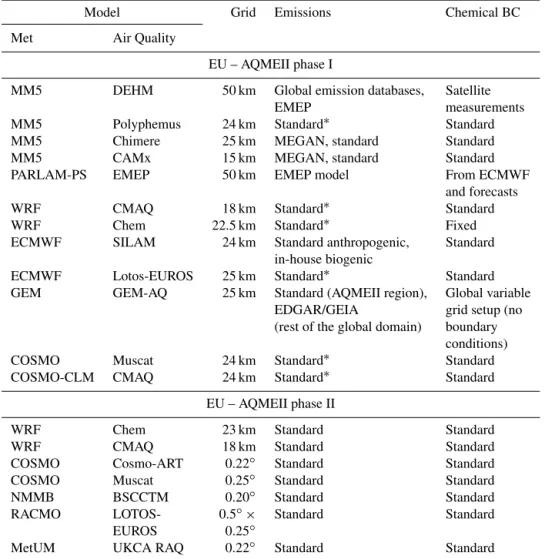
Table 1.The modelling systems participating in the first and second phases of AQMEII for Europe.
Model Grid Emissions Chemical BC
Met Air Quality
EU – AQMEII phase I
MM5 DEHM 50 km Global emission databases, Satellite
EMEP measurements
MM5 Polyphemus 24 km Standard∗ Standard
MM5 Chimere 25 km MEGAN, standard Standard
MM5 CAMx 15 km MEGAN, standard Standard
PARLAM-PS EMEP 50 km EMEP model From ECMWF
and forecasts
WRF CMAQ 18 km Standard∗ Standard
WRF Chem 22.5 km Standard∗ Fixed
ECMWF SILAM 24 km Standard anthropogenic, Standard
in-house biogenic
ECMWF Lotos-EUROS 25 km Standard∗ Standard
GEM GEM-AQ 25 km Standard (AQMEII region), Global variable
EDGAR/GEIA grid setup (no
(rest of the global domain) boundary conditions)
COSMO Muscat 24 km Standard∗ Standard
COSMO-CLM CMAQ 24 km Standard∗ Standard
EU – AQMEII phase II
WRF Chem 23 km Standard Standard
WRF CMAQ 18 km Standard Standard
COSMO Cosmo-ART 0.22◦ Standard Standard
COSMO Muscat 0.25◦ Standard Standard
NMMB BSCCTM 0.20◦ Standard Standard
RACMO LOTOS- 0.5◦× Standard Standard
EUROS 0.25◦
MetUM UKCA RAQ 0.22◦ Standard Standard
AQMEII phase I: Standard boundary conditions, provided from GEMS project (Global and regional Earth-system Monitoring using Satellite and in situ data). Refer to Schere et al. (2012) for details.∗Standard anthropogenic emissions and biogenic emissions derived from meteorology (temperature and solar radiation) and land use distribution implemented in the meteorological driver. Refer to Solazzo et al. (2012a, b) and references therein for details.
AQMEII phase II: Standard boundary conditions, 3-D daily chemical boundary conditions were provided by the ECMWF IFS-MOZART model run in the context of the MACC–II project (Monitoring Atmospheric Composition and Climate – Interim Implementation) every 3 h and 1.125 spatial resolution. Refer to Im et al. (2015a, b) for details. Standard emissions, based on the TNO-MACC-II (Netherlands Organization for Applied Scientific Research, Monitoring Atmospheric Composition and Climate – Interim Implementation) framework for Europe. Refer to Im et al. (2015a, b) for details.
3 Setup: experiments, models and observations
The two AQMEII ensemble datasets have simulated the air quality for Europe (10◦W–39◦E, 30–65◦N) and North America (125–55◦W, 26–51◦N. Despite the common do-mains, the modelling systems across the two phases have profound differences. The simulation year was 2006 for AQMEII-I and 2010 for AQMEII-II; therefore, the two sets are dissimilar with respect to the input data (emissions, chemical boundary conditions, meteorology). Boundary con-ditions are obtained from GEMS (Global and Regional Earth-System Monitoring using Satellite and in situ data) in AQMEII-I and MACC (Monitoring Atmospheric Compo-sition and Climate) in AQMEII-II. The air quality models
of the second phase are coupled with their meteorological driver (chemistry feedbacks on meteorology), while those of the first phase are not. The participating models are also dif-ferent. Detailed analysis of the emissions, boundary condi-tions and meteorology for the modelled year 2006 (AQMEII-I) is presented in Pouliot et al. (2012), Schere et al. (2012) and Vautard et al. (2012). For 2010 (AQMEII-II), similar in-formation is presented in Pouliot et al. (2015), Giordano et al. (2015) and Brunner et al. (2015).
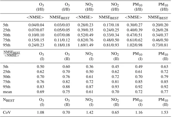
meteo-Table 2. The statistical distribution of (a) the normalized mean square error (NMSE) of the best model (NMSEBEST), (b) the ensem-ble average NMSE (<NMSE>) and (c) the skill difference indicator (NMSEBEST/<NMSE>). In addition, the coefficient of variation
(CoV=standard deviation divided by the mean) of the number of cases where each model was identified as best is shown. All indicators were evaluated at each monitoring site for the examined species of the two AQMEII phases.
O3 O3 NO2 NO2 PM10 PM10
(I/II) (I/II) (I/II) (I/II) (I/II) (I/II)
<NMSE> NMSEBEST <NMSE> NMSEBEST <NMSE> NMSEBEST
5th 0.04/0.04 0.03/0.03 0.28/0.23 0.17/0.18 0.30/0.27 0.20/0.20
25th 0.07/0.07 0.05/0.05 0.39/0.35 0.24/0.25 0.40/0.39 0.26/0.28
50th 0.10/0.10 0.07/0.08 0.52/0.49 0.33/0.34 0.47/0.51 0.34/0.37
75th 0.15/0.15 0.11/0.12 0.82/0.76 0.48/0.50 0.61/0.62 0.46/0.50
95th 0.24/0.23 0.18/0.18 1.69/1.49 0.81/0.93 1.02/0.98 0.73/0.81
NMSEBEST
<NMSE> O3 O3 NO2 NO2 PM10 PM10
(I) (II) (I) (II) (I) (II)
5th 0.50 0.60 0.36 0.45 0.49 0.63
25th 0.62 0.70 0.50 0.62 0.61 0.72
50th 0.70 0.76 0.61 0.72 0.70 0.79
75th 0.76 0.82 0.72 0.81 0.85 0.85
95th 0.83 0.88 0.87 0.93 0.92 0.92
mean 0.69 0.75 0.61 0.70 0.72 0.77
NBEST O3 O3 NO2 NO2 PM10 PM10
(I) (II) (I) (II) (I) (II)
CoV 1.08 0.70 1.42 0.65 1.16 1.53
rological analysis. In AQMEII-II, the simulations were run more in a way as if they were real forecasts; meteorologi-cal boundary conditions for the majority of the models were from the ECMWF operational archive (see Tables 1 and 2 in Brunner et al., 2015), and no nudging or FDDA (four-dimensional data assimilation) was applied. However, the driving meteorological data were analysis (but no reanalysis) for all simulations, with exception of the COSMO-MUSCAT run. Hence, the runs from AQMEII-II are more like forecasts than those from AQMEII-I.
Recent studies with regional air quality models yielded that the full variability of the ensemble can be retained with only an effective number of models (NEFF) on the order of 5–
6 (e.g. Solazzo et al., 2013; Kioutsioukis and Galmarini, 2014; Marécal et al., 2015). The minimum number of en-semble members to sample the uncertainty should be well above NEFF; for this reason, we focus on the European
do-main (EU) due to its sufficient number of models for forming the ensemble.
Table 1 summarizes the features of the modelling systems analysed in this study with regard to O3, NO2and PM10
con-centrations in the EU. The modelling contribution to the two phases of AQMEII consists of 12, 13 and 10 models for O3,
NO2and PM10respectively in AQMEII-I, while 14 members
were available for all species in AQMEII-II. Several discrete simulations of WRF-Chem with alternative chemistry and
physics configurations are included in AQMEII-II (Forkel et al., 2015; San José et al., 2015; Baró et al., 2015).
Following the statements of Sect. 2, each model was bias-corrected prior to the analysis, i.e. its own mean bias over the examined 3-month period was subtracted from its mod-elled time series at each monitoring site. For each modelling system, its long-term systematic error is a known quantity estimated during its validation stage; therefore, the subtrac-tion of the seasonal bias does not restrict the generality of the study. Actually, the requirement for bias removal is a neces-sary condition only for the weighted ensemble mean. In the results section we will address this issue and its effect on the skill of the ensemble estimators.
The observational datasets for O3, NO2and PM10derived
from the surface Air Quality monitoring networks operating in the EU constitute the same dataset used in the first and second phases of AQMEII to support model evaluation. All monitoring stations are rural and have data at least 75 % of the time. The network is denser for O3(451 and 450 stations
in AQMEII-I and II) for which there are as many monitor-ing stations as for NO2(290 and 337 stations in AQMEII-I
and II) and PM10(126 and 131 stations in AQMEII-I and II)
combined, with PM10 having the fewest observations.
CD
F
Concentration (ug m3 )-1
Figure 1.The cumulative density functions of the observations (O3, NO2, PM10) in the two AQMEII phases (Phase I: filled circles, Phase II: unfilled circles). Each bullet represents the median at the specific percentile.
(Massey, 1951) yields that only the PM10distributions differ
at the 1 % significance level. This results from the unavail-ability of data for France and the UK in AQMEII-II for PM10
(station locations are shown in Fig. 3).
4 Results
In this section we apply the conceptual context briefly pre-sented in Sect. 2 to investigate the effect of the differences in the ensemble properties within each of the two AQMEII phases (Rao et al., 2011) in the skill of the unconditional multi-model mean. The potential for improved estimates through conditional ensemble averages and their robustness is ultimately assessed.
From the station-based hourly time series provided, we analysed one season (3-month period) with continuous data and relatively high concentrations: for O3, June–July–
August was selected, while September–October–November was used for NO2and PM10.
4.1 Single models
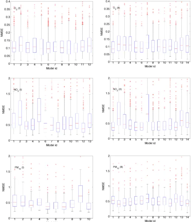
The distributions of each model’s NMSE for O3, NO2and
PM10 over all monitoring stations are presented in Fig. 2
as box-and-whisker plots. On each box, the central mark indicates the median, and the bottom and top edges of the box indicate the 25th and 75th percentiles respectively. The whiskers extend to the most extreme data points not con-sidered outliers (i.e. points with distance from the 25th and 75th percentiles smaller than 1.5 times the interquartile range). Among the examined pollutants, the models simu-late the O3concentrations better, as is evident from the axis
scale. The highest variability in the skill between and within the models is observed for NO2.
The distribution of average NMSE at each sta-tion (<NMSE>) has a median on the order of 0.1 for
O3 and 0.5 for NO2 and PM10 for both phases (Table 2).
The application of the Kolmogorov–Smirnov test (Massey, 1951) to the<NMSE>distributions across AQMEII-I and
AQMEII-II shows that there are no statistically significant differences in the<NMSE>distributions between the two
ensemble datasets at the 1 % significance level. The same also applies for the statistical distribution of the minimum NMSE at each station (NMSEBEST) at each monitoring
station. Hence, despite the different modelling systems and input data, the <NMSE> and NMSEBEST distributions
between AQMEII-I and AQMEII-II are indistinguishable for the three examined pollutants.
Aside from<NMSE>and NMSEBEST, we evaluate the
percentage of cases each model identified as being “best” and calculate the coefficient of variation (CoV=std/mean) of this index for each ensemble. If models were behaving like i.i.d., the probabilities of being best would be roughly equal (∼1/M) for all models and the CoV would generally be well
below unity for the examined range of ensemble members. As can be inferred from Table 2, the proportion ofequally good modelsis higher for O3and NO2in the second dataset.
Among the pollutants, the CoV of NO2exhibits the most
dra-matic change.
4.2 Pitfalls of the unconditional multi-model mean
The skill of the multi-model mean was compared to the skill of the best deterministic model, independently evaluated at each monitoring site (hereafter bestL). The geographical dis-tribution of the ratio RMSE(mme)/RMSEBESTMODELis
pre-sented in Fig. 3. The indicator does not exhibit any longitu-dinal or latitulongitu-dinal dependence. Summary statistics indicate that the mme outscores the bestL at roughly half of the sta-tions for O3(namely 52 and 49 for AQMEII-I and II) and
at approximately 40 % of the stations for PM10 (38 and 42).
The same statistic for NO2varies considerably (39 and 64).
The Kolmogorov–Smirnov test yields that the corresponding distributions (pI and pII) are different at the 1 % significance level, but thet test demonstrates that the mean of the
distri-butions differ significantly only for NO2. The reason behind
the skill of mme with respect to the bestL is investigated next with respect to the skill difference and the error dependence of each ensemble.
The skill difference between the best model and the average skill is inferred from the indicator NMSEBEST/<NMSE> (Table 2). High values of the
indicator correspond to small skill differences between the ensemble members (desirable). The distribution of the NMSEBEST/<NMSE>at each station has a median on the
the pollutant. The spread of the indicator, measured by its interquartile range, is higher for NO2and lower for O3.
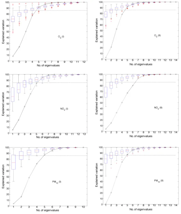
The eigenvalues of the covariance matrix calculated from the model errors provide information on the member diver-sity and the ensemble redundancy (Eq. 5). Following the eigenanalysis of the error covariance matrix at each sta-tion separately and converting the eigenvalues to cumula-tive amount of explained variance, the resulting matrix is presented in a box and whisker plot (Fig. 4). The error de-pendence of the ensemble members is deduced from the ex-plained variation by the maximum eigenvaluesm. Low
val-ues of the indicator correspond to independent members with small error dependence (desirable). The average variation ex-plained bysmranges between 65 and 79 %, taking the lower
values for NO2. The spread of the indicator, measured by its
interquartile range, is higher for NO2and lower for O3.
All species demonstrate smaller skill difference and higher error dependence in the AQMEII-II dataset. The Kolmogorov–Smirnov test yielded that the difference in the corresponding distributions of the indicators between AQMEII-I and AQMEII-II is significant at the 1 % level. However, it is the joint distribution of skill difference and error dependence that modulates the mme skill with respect to the bestL, as seen in Fig. 5. Shifts in the distributions of the indicators at opposite directions eventually cancel out, yield-ing no change in the mme skill. This case is observed for O3
and PM10. For NO2, skill difference was improved more than
error dependence was worsened, yielding a net improvement of mme in AQMEII-II.
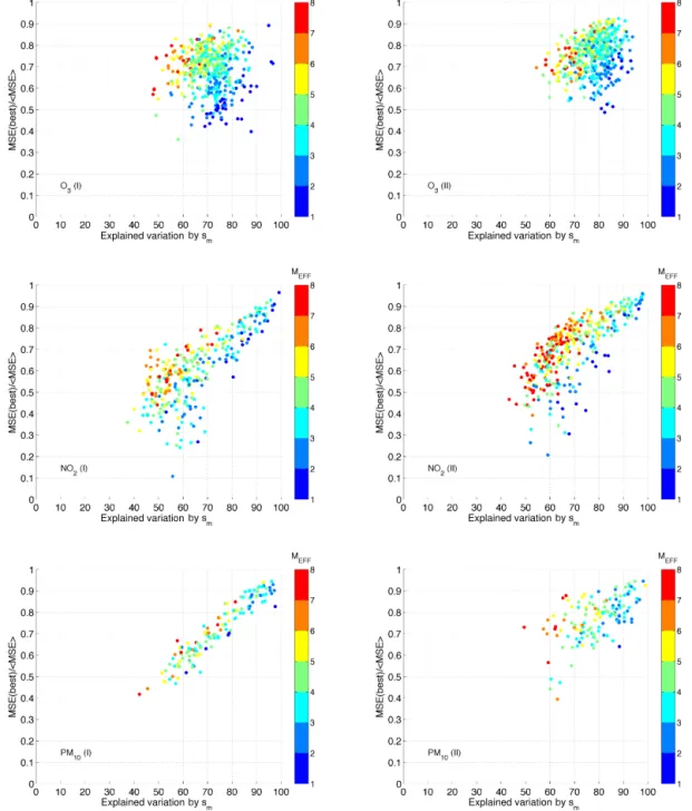
The area below the diagonal in Fig. 5 corresponds to mon-itoring sites with disproportionally low diversity under the current level of accuracy. This area of the chart indicates high spread in skill difference and relatively highly depen-dent errors. This situation practically means a limited num-ber of skilled models with correlated errors, which in turn denotes a smallNEFFvalue, as demonstrated in Fig. 6. The
opposite state is true for the area above the diagonal. It cor-responds to locations that are constituted from models with comparable skill and relatively independent errors, reflecting a highNEFFvalue. This matches the desired synthesis for an
ensemble.
The cumulative distribution ofNEFFfrom the error
mini-mization (i.e. the optimal trade-off between accuracy and di-versity) across all possible combinations of M models at each site is also presented in Fig. 4 (solid line). At over 90 % of the stations, we do not need more than five members for O3,
six members for PM10 and six to seven members for NO2.
Furthermore, from a pool of 10–14 models, the benefits of ensemble averaging cease after five to seven members (but not five to seven particular members across all stations).
4.3 Conditional multi-model mean
Following the identification of the weaknesses in the ensem-ble design, the potential for corrections through more
so-phisticated schemes is now investigated. We consider the skill of the multi-model mean as the starting point, and we investigate pathways for further enhancing it through the non-trivial problem of weighting or sub-selecting. The opti-mal weights (mmW) are estimated from the analytical for-mulas presented in Potempski and Galmarini (2009). The sub-selection of members was built upon the optimization of either the accuracy–diversity trade-off (mme<)
(Kiout-sioukis and Galmarini, 2014) or the spectral representation of first-order components from different models (kzFO) (Gal-marini et al., 2013). Another approach built upon higher or-der (namely,NEFF) spectral components (kzHO) is also
in-vestigated. In this section we mark the boundaries of the possible improvements for different ensemble mean estima-tors applicable to the AQMEII datasets and their sensitivity to suboptimal conditions using cross-validation.
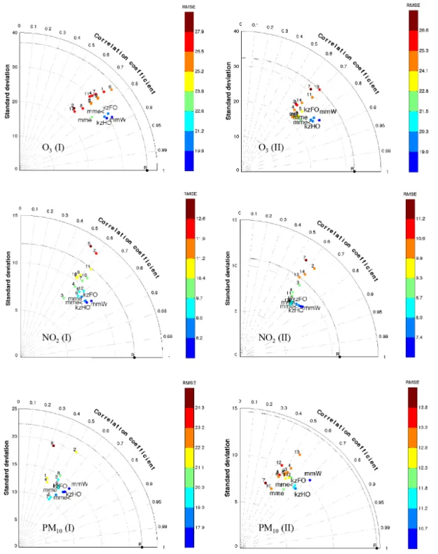
The global skill of all the single models and the ensem-ble estimators, evaluated at all stations, is presented in Fig. 7 in the form of Taylor plots. For O3, the deterministic
mod-els have standard deviations that are smaller compared to observations and a narrow correlation pattern (∼0.7) that is slightly deteriorated in AQMEII-II. For NO2, members with
higher and lower variance than the observed variance exist in the ensemble, while the correlation spread becomes nar-rower in AQMEII-II and demonstrates a minor improvement. Last, simulated PM10from the deterministic models displays
smaller standard deviation compared to observations with a wide correlation spread (0.3–0.6). The multi-model mean is always found closer to the reference point, in an area that in-corporates lower error and increased correlation but at the same time generally low variance. The examined ensem-ble estimators (mmW, mme<, kzFO, kzHO) are horizontally
shifted from mme; hence, they demonstrate even lower er-ror and increased correlation and variance. Among them, the highest composite skill was found for mmW, followed by kzHO.
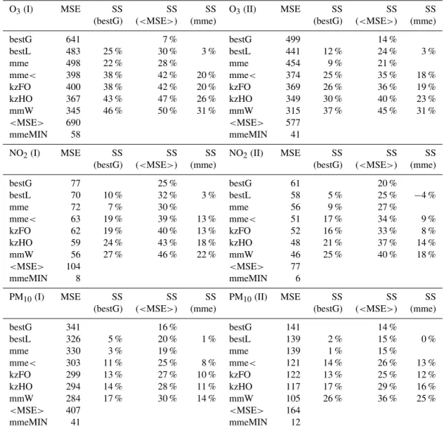
A comparison between the skill of the examined ensem-ble estimators versus the mme and the best single model is now conducted (Table 3). The best single model is evaluated globally (bestG is the average across all stations) and locally (bestL is at each station separately). The former estimates the best average deterministic skill among the candidate models; the latter provides a useful indicator for controlling whether the anticipated benefits of ensemble averaging holds. The skill scores were evaluated against the guaranteed minimum gain of the ensemble (<MSE>), the ensemble mean (mme)
and the best single model globally (bestG). The estimations calculated from the unprecedented AQMEII datasets (2 years of hourly measurements and simulations from two different ensembles of 10–14 models each at over 450 stations for three pollutants) allows the following interpretation:
– The mme always achieves a lower error than bestG. The advancement is higher for O3 (9–22 %), followed
Figure 2.Model skill difference via the NMSE. For each box, the central mark indicates the median, and the bottom and top edges of the box indicate the 25th and 75th percentiles respectively. The whiskers extend to the most extreme data points not considered outliers and the outliers (points with distance from the 25th and 75th percentiles larger than 1.5 times the interquartile range) are plotted individually using the “+” symbol.
skill improvement (1–3 %). With respect to bestL, the mme generally attains similar or slightly higher MSE. Hence, the average error over multiple stations statisti-cally favours the ensemble mean over the single models but the comparison at each site generally does not as it depends on the skill difference and the error dependence of the models.
– The skill score of mme over<MSE>(i.e. the
guaran-teed upper ceiling for the MSE of mme, from Eq. 2) ranges between 15 and 30 %, higher for NO2and lower
for PM10. According to Eq. (2), this number also
Figure 3.Comparison of the mme skill against the best local deterministic model by means of the indicator RMSEMME/RMSEBEST.
– The skill score of the examined ensemble estimators (mmW, mme<, kzFO, kzHO) over<MSE>ranges
be-tween 25 and 50 %, higher for O3 and NO2and lower
for PM10. Among them, the improvement is higher for
mmW and lower for mme<and kzFO. Thus, the
pro-motion of accuracy and diversity within the ensemble almost doubles the distance to <MSE>compared to
mme and results in an additional skill over the mme be-tween 14 and 31 % (for mmW).
– The improvement of the ensemble estimator using se-lectedNEFFmembers (mme<) over all members (mme)
is illustrated in Fig. 8 in the context of skill differ-ence and error dependdiffer-ence. The charts demonstrate no points below the diagonal, i.e. the sub-selection results in an ensemble constituted from models with compara-ble skill and relatively independent errors (compared to the full ensemble).
Figure 4.Model error dependence through the eigenvalues spectrum. The average explained variation from the maximum eigenvalue is 71 and 78 (phase I and II) for O3, 65 and 69 for NO2and 74 and 79 for PM10. On the same graph, the cumulative density function ofNEFF calculated from all possible ensemble combinations is presented with the black line.
The statistical distributions of the skill scores of the ex-amined ensemble estimators (mmW, mme<, kzFO, kzHO)
over mme are well bounded from higher than unity values to lower than unity values (Fig. 9). The only exception ex-ists for roughly 10 % of the stations for all pollutants, where kzFO demonstrates higher MSE compared to mme. Unlike the other ensemble estimators, kzFO utilizes independent spectral components, each obtained from a single model, eliminating the possibility for “cancelling out” of random
er-rors. All cases belonging to this 10 % of the samples (lower tail of the cdf) demonstrate highNEFF, where the benefits
from unconditional ensemble averaging are optimal (Kiout-sioukis and Galmarini, 2014). Conversely, for another 10 % of the stations (upper tail of the cdf), there is an abrupt im-provement from the conditional ensemble estimators. Those cases demonstrate lowNEFF, where the benefits from
Explained variation Explained variation
Explained variation Explained variation
Explained variation Explained variation
Figure 5.Interpretation of Fig. 3: the explanation of the mme skill against the best local deterministic model with respect to skill difference (evaluated from MSEBEST/<MSE>) and error dependence (evaluated from the explained variation by the highest eigenvalue).
The ability to simulate extreme values is now examined through the POD and FAR indices. Two thresholds were uti-lized for each pollutant, being 120 and 180 µg m−3for O
3,
25 and 50 µg m−3for NO
2, and 50 and 90 µg m−3for PM10.
The average 90th percentile across the stations was 129 and 117 µg m−3(AQMEII-I and II) for O
3, 30 and 26 µg m−3for
NO2 and 52 and 33 µg m−3 for PM10 (Fig. 1). Hence, the
thresholds fall into the upper 10 % of the distributions, being even more extreme for PM10in AQMEII-II. The numbers in
Table 4 give rise to the following inferences:
– For O3and NO2, mme achieves somewhat higher POD
than bestG at the lower threshold, but the order is re-versed at the higher threshold. For PM10, bestG
al-ways performs better than mme for values exceeding the lower threshold. As we move towards the tail, the POD of bestG dominates over the mme. Thus, the rank-ing of mme and bestG at the extreme percentiles and on average (seen earlier) are opposite.
– The mme<generally achieves somewhat higher POD
re-Explained variation Explained variation
Explained variation Explained variation
Explained variation Explained variation
Figure 6.Like Fig. 5 but showing theNEFFwith respect to skill difference and error dependence.
versed at the higher threshold. Over that level, kzFO and mmW are the only estimators with POD higher than bestL.
– As we move towards higher percentiles, the first-order spectral model (kzFO) has higher POD than the higher-order spectral model (kzHO) due to the averaging in the latter. In addition, the frequency domain averag-ing (kzHO) had slightly higher POD compared to the time domain averaging (mme<).
– The mmW, aside from its lower MSE, has the highest POD among all models and ensemble estimators.
– The variation of FAR was very small between all exam-ined models and ensemble estimators.
The combination of the results from the average error and the extremes identify mmW as the estimator that outscores the others across all percentiles. kzFO has a high capacity for extremes but requires attention for the limited sites with high
Figure 7.Composite skill of all deterministic models and ensemble estimators (mme, mme<, kzFO, kzHO, mmW) through Taylor plots. The pointRrepresents the reference point (i.e. observations).
have both high skill across all percentiles (better for kzHO), but they could have inferior POD compared to bestL at the extreme percentiles. With respect to the pollutants, the ad-vancement of mmW skill over mme was higher for O3.
The additional skill over mme in the range between 8 and 31 % from the statistical approaches applied to a pool of en-semble simulations identifies the upper ceiling of the
Table 3.The MSE from (a) the best deterministic models globally (bestG) and locally (bestL), (b) the unconditional ensemble mean (mme), and (c) the four conditional ensemble estimators (mme<, kzFO, kzHO, mmW). In addition, the bounds for the MSE of the ensemble mean
are also presented. The maximum value (<MSE>) arises for ensemble members without diversity and the minimum value (mmeMIN) was
estimated from the variance term only (i.e. calculated for unbiased and uncorrelated ensemble members). The ability of the estimators is evaluated through their skill scores (SSREF=1−MSE/MSEREF, REF=bestG,<MSE>, mme).
O3(I) MSE SS SS SS O3(II) MSE SS SS SS
(bestG) (<MSE>) (mme) (bestG) (<MSE>) (mme)
bestG 641 7 % bestG 499 14 %
bestL 483 25 % 30 % 3 % bestL 441 12 % 24 % 3 %
mme 498 22 % 28 % mme 454 9 % 21 %
mme< 398 38 % 42 % 20 % mme< 374 25 % 35 % 18 %
kzFO 400 38 % 42 % 20 % kzFO 369 26 % 36 % 19 %
kzHO 367 43 % 47 % 26 % kzHO 349 30 % 40 % 23 %
mmW 345 46 % 50 % 31 % mmW 315 37 % 45 % 31 %
<MSE> 690 <MSE> 577
mmeMIN 58 mmeMIN 41
NO2(I) MSE SS SS SS NO2(II) MSE SS SS SS
(bestG) (<MSE>) (mme) (bestG) (<MSE>) (mme)
bestG 77 25 % bestG 61 20 %
bestL 70 10 % 32 % 3 % bestL 58 5 % 25 % −4 %
mme 72 7 % 30 % mme 56 9 % 27 %
mme< 63 19 % 39 % 13 % mme< 51 17 % 34 % 9 %
kzFO 62 19 % 40 % 13 % kzFO 52 16 % 33 % 8 %
kzHO 59 24 % 43 % 18 % kzHO 48 21 % 37 % 14 %
mmW 56 27 % 46 % 22 % mmW 46 25 % 40 % 18 %
<MSE> 104 <MSE> 77
mmeMIN 8 mmeMIN 6
PM10(I) MSE SS SS SS PM10(II) MSE SS SS SS
(bestG) (<MSE>) (mme) (bestG) (<MSE>) (mme)
bestG 341 16 % bestG 141 14 %
bestL 326 5 % 20 % 1 % bestL 139 2 % 15 % 0 %
mme 330 3 % 19 % mme 139 1 % 15 %
mme< 303 11 % 25 % 8 % mme< 121 14 % 26 % 13 %
kzFO 299 13 % 27 % 10 % kzFO 122 13 % 25 % 12 %
kzHO 294 14 % 28 % 11 % kzHO 117 17 % 29 % 16 %
mmW 284 17 % 30 % 14 % mmW 105 26 % 36 % 25 %
<MSE> 407 <MSE> 164
mmeMIN 41 mmeMIN 12
mme: unconditional ensemble mean; mme<: conditional ensemble mean (Kioutsioukis and Galmarini, 2014); kzFO: conditional spectral ensemble mean with first-order components (Galmarini et al., 2013); kzHO: conditional spectral ensemble mean with second- and higher-order components (kzHO); mmW: optimal weighted ensemble (Potempski and Galmarini, 2009).
on the training set for variable time series length that is pro-gressively increasing from 1 to 60 days, for all monitoring stations and pollutants. The evaluation period for all train-ing windows is the same 30-day segment, not available in the training procedure. The analysis will provide a perspec-tive on applying the techniques in a forecasting context, al-though the examined simulations did not operate in forecast-ing mode.
The interquartile range of the day-to-day difference in the weights is calculated and its range over all stations is dis-played in Fig. 10. No convergence occurs; however, the
vari-ability of the mmW weights is notably reduced after a certain amount of time. If we set a tolerance level at the second dec-imal, to be satisfied at all stations, we need at a minimum 20–45 days of hourly time series. The variability of weights is smaller for O3 and higher for NO2and PM10, explained
by the larger NMSE spread in the latter case. The identifi-cation of the necessary training or learning period will be assessed by its effect on the mmW skill. Table 5 presents the mmW skill obtained from training over time series of differ-ent lengths varying from 5 to 60 days. For O3, mmW trained
Explained variation Explained variation
Explained variation Explained variation
Explained variation Explained variation
Figure 8.Like Fig. 5 but for the mme<skill in the reduced ensemble. Please note the change in the colour scale.
periods result in large departures from mme. NO2and PM10
require larger training periods than O3. The use of mmW is
practically of no benefit compared to mme if the training pe-riod is less than 20 days for NO2and 30 days for PM10. For
all pollutants, the variability of the weights and the bias have no effect on the error after 60 days.
The results demonstrate that the ensemble estimators based on the analytical optimization become insensitive to inaccuracies in the bias and weights for training peri-ods exceeding 60 days. However, other published studies with weighted ensembles using non-analytical optimization
(e.g. linear regression; Monteiro et al., 2013), argue that 1 month is sufficient for the weights and the bias. The sub-selecting schemes are more robust compared to the optimal weighting scheme in the variations of their parameters (bias, members). Using data from AQMEII-I, training periods in the order of 1 week were found essential for mme<
Figure 9.The cumulative density function of the skill score (1−MSEX/MSEMME,X=mmW, mme<, kzFO, kzHO) over mme, evaluated
at each monitoring site for the examined species of the two AQMEII phases.
5 Conclusions
In this paper we analyse two independent suites of chemi-cal weather modelling systems regarding their effect on the skill of the ensemble mean (mme). The results are interpreted with respect to the error decomposition of the mme. Four ways to extract more information from an ensemble aside from the mme are ultimately investigated and evaluated. The first approach applies optimal weights to the models of the ensemble (mmW), and the other three methods utilize
se-lected members in time (mme<) or frequency (kzFO, kzHO)
domain. The study focuses on O3, NO2and PM10, using the
unprecedented datasets from two phases of AQMEII over the European domain.
The comparison of the mme skill versus the globally best single model (bestG is identified from the evaluation over all stations) points out that mme achieves lower average (across all stations) error compared to bestG. The enhancement of accuracy is highest for O3(up to 22 %) and lowest for PM10
en-Table 4.The probability of detection (POD) and false alarm rate (FAR) from (a) the best deterministic models, globally (bestG) and lo-cally (bestL), (b) the unconditional ensemble mean (mme), and (c) the four conditional ensemble estimators (mme<, kzFO, kzHO, mmW).
Two thresholds were examined for each indicator, corresponding to tail percentiles.
O3(I) POD FAR POD FAR O3(II) POD FAR POD FAR
threshold 120 180 threshold 120 180
bestG 37.9 3.6 11.4 0.0 bestG 19.9 1.2 1.2 0.0
bestL 54.7 3.5 19.5 0.0 bestL 33.2 1.5 5.4 0.0
mme 39.9 2.5 12.0 0.0 mme 22.0 1.2 0.5 0.0
mme< 53.5 2.6 18.3 0.0 mme< 34.9 1.3 2.4 0.0
kzFO 57.7 3.0 19.6 0.0 kzFO 39.1 1.5 4.4 0.0
kzHO 57.1 2.5 19.2 0.0 kzHO 36.9 1.2 2.3 0.0
mmW 60.6 2.6 27.2 0.0 mmW 45.4 1.6 8.6 0.0
NO2(I) POD FAR POD FAR NO2(II) POD FAR POD FAR
threshold 25 50 threshold 25 50
bestG 45.9 4.6 3.8 0.2 bestG 39.3 3.3 4.9 0.1
bestL 48.7 4.2 8.5 0.3 bestL 41.4 3.1 8.1 0.1
mme 49.4 4.6 3.0 0.1 mme 44.4 3.5 5.4 0.1
mme< 52.2 4.1 7.1 0.1 mme< 47.6 3.2 7.6 0.1
kzFO 52.7 4.1 8.4 0.1 kzFO 46.5 3.1 9.5 0.1
kzHO 54.2 4.0 6.8 0.1 kzHO 49.5 3.2 9.3 0.1
mmW 57.0 4.1 14.8 0.2 mmW 50.9 3.1 13.5 0.1
PM10(I) POD FAR POD FAR PM10(II) POD FAR POD FAR
threshold 50 90 threshold 50 90
bestG 25.9 2.7 1.2 0.0 bestG 13.0 0.4 0.0 0.0
bestL 27.8 2.3 6.9 1.2 bestL 14.5 0.4 1.6 0.0
mme 21.6 1.8 0.4 0.0 mme 11.4 0.4 0.0 0.0
mme< 30.6 2.3 5.6 0.1 mme< 13.9 0.4 0.0 0.0
kzFO 31.1 2.3 6.9 0.1 kzFO 14.1 0.3 0.0 0.0
kzHO 33.2 2.4 6.1 0.1 kzHO 13.2 0.3 0.2 0.0
mmW 35.5 2.6 13.3 0.2 mmW 23.9 0.4 20.8 0.0
mme: unconditional ensemble mean; mme<: conditional ensemble mean (Kioutsioukis and Galmarini, 2014); kzFO: conditional spectral ensemble mean with first-order components (Galmarini et al., 2013); kzHO: conditional spectral ensemble mean with second- and higher-order components (kzHO); mmW: optimal weighted ensemble (Potempski and Galmarini, 2009).
Table 5.The average MSE of mmW for various training lengths, calculated for the testing time series (i.e. not used in the training phase) that contains all stations.
Length of O3 O3 NO2 NO2 PM10 PM10
training (I) (II) (I) (II) (I) (II)
period (days)
5 616 540 90 91 717 210
10 496 441 77 66 443 150
20 400 378 65 56 348 125
30 380 344 62 52 308 109
40 366 334 59 50 300 113
50 357 326 57 48 294 108
60 351 319 56 45 282 102
semble averaging of air quality time series holds at each sta-tion by directly comparing the mme and the locally best sin-gle model (bestL: identified from the evaluation at each sta-tion). Summary statistics indicate that the mme outscores the bestL at roughly 50 % of the stations for O3and at
approx-imately 40 % of the stations for PM10, while for NO2 the
values were about 40 and 60 % for the two datasets. This re-sult indicates that there are a considerable number of stations (over 40 %) where the unconditional averaging is not advan-tageous because the ensemble does not meet the necessary conditions. A new chart is introduced in this paper that in-terprets the skill of the mme according to the skill difference and the error dependence of the ensemble members.
Time series length (days) Time series length (days)
Time series length (days) Time series length (days)
Time series length (days) Time series length (days)
Weight difference Weight difference
Weight difference Weight difference
Weight difference Weight difference
Figure 10.The interquartile range over all stations of the day-to-day difference in the weights arising from variable time series length.
– The skill score of mme over its guaranteed upper ceil-ing (case of zero diversity) ranges between 15 and 30 %, being lower for PM10. Those percentages also
repre-sent the diversity normalized by the accuracy. There-fore, aside from improving the single models, their com-bination in an ensemble confines the mme skill if their diversity is limited.
– The promotion of the right amount of accuracy and di-versity in the conditional ensemble estimators almost doubles the distance to the guaranteed upper ceiling. The skill score over mme is higher for O3(in the range
of 18–31 %) and lower for NO2and PM10(in the range
– The theoretical minimum MSE of mme for the case of unbiased and uncorrelated models is far from being achieved from all ensemble estimators.
– As we move towards the tail, the probability of detec-tion (POD) of bestG (bestL) dominates over the mme (mme<). At the extreme percentiles, kzFO and mmW
are the only estimators with POD higher than bestL. – The combination of the results from the average error
and the extremes identifies mmW as the estimator that outscores the others across all percentiles. kzFO has a high capacity for extremes but requires attention for the limited sites with highNEFF, where its skill is inferior to
mme. kzHO and mme<have both high skill across all
percentiles (better for kzHO), but they could have infe-rior POD compared to bestL at the extreme percentiles. The skill enhancement is superior using the weighting scheme but the required training period to acquire repre-sentative weights was longer compared to the sub-selecting schemes. For all pollutants, the variability of the weights and the bias has negligible effect on the error for training peri-ods longer than 60 days. For the schemes relying on mem-ber selection, accurate recent representations on the order of a week were sufficient. The learning periods constitute the necessary time for acquiring similar prior and posterior dis-tributions in the controlling parameters of samples. The risks of all the statistical learning processes originate from the vi-olation of this assumption, which holds in the case of chang-ing weather or chemical regimes for example. Therefore, the operational implementation of each ensemble approach re-quires knowledge of its safety margins for the examined pol-lutants as well as its risks.
The improvement of the physical, chemical and dynamical processes in the deterministic models is a continuous proce-dure that results in better forecasts. Furthermore, mathemat-ical optimizations in the input data (e.g. data assimilation) or the model output (e.g. ensemble estimators) have a sig-nificant contribution in the accuracy of the whole modelling process. The presented post-simulation advancements were the result only of favourable ensemble design. However, the theoretical minimum MSE of mme for the case of unbiased and uncorrelated models is far from being achieved from all ensemble estimators. Further development is underway in the presented ensemble methods that take into account the mete-orological and chemical regimes.
6 Data availability
Appendix A: Spectral decomposition
The relevant separate scales of motion are defined by means of physical considerations and periodogram analysis (Rao et al., 1997). They are namely the intraday component (ID), the diurnal component (DU), the synoptic component (SY) and the long-term component (LT). The hourly time series (S)
can therefore be decomposed as
S(t )=ID(t )+DU(t )+SY(t )+LT(t ), (A1)
where
ID(t )=S(t )−KZ3,3
DU(t )=KZ3,3−KZ13,5 SY(t )=KZ13,5−KZ103,5
LT(t )=KZ103,5. (A2)
The Kolmogorov–Zurbenko (KZ) filter is defined as an itera-tion of a moving-average filter applied on a time-seriesS(t ).
It is controlled by the window size (m) and the number of
iterations (p):
KZm,p=Rpi=1
JWi
k=1
1
m
m−1
2
X
j=−m−21
S(ti)k,j
R: iteration
J: running window
Wi =Li−m+1
Li=length ofS (ti)
Acknowledgements. We gratefully acknowledge the contribution
of various groups to the second Air Quality Model Evaluation international Initiative (AQMEII) activity: US EPA, Environ-ment Canada, Mexican Secretariat of the EnvironEnviron-ment and Natural Resources (Secretaría de Medio Ambiente y Recursos Naturales-SEMARNAT) and National Institute of Ecology (In-stituto Nacional de Ecología-INE) (North American national emissions inventories); US EPA (North American emissions pro-cessing); TNO (European emissions propro-cessing); ECMWF/MACC project & Météo-France/CNRM-GAME (Chemical boundary conditions). Ambient North American concentration measurements were extracted from Environment Canada’s National Atmospheric Chemistry Database (NAtChem) PM database and provided by several US and Canadian agencies (AQS, CAPMoN, CASTNet, IMPROVE, NAPS, SEARCH and STN networks); North Amer-ican precipitation-chemistry measurements were extracted from NAtChem’s precipitation-chemistry database and were provided by several US and Canadian agencies (CAPMoN, NADP, NBPMN, NSPSN, and REPQ networks); the WMO World Ozone and Ultraviolet Data Centre (WOUDC) and its data-contributing agencies provided North American and European ozone sonde profiles; NASA’s Aerosol Robotic Network (AeroNet) and its data-contributing agencies provided North American and European AOD measurements; the MOZAIC Data Centre and its contributing airlines provided North American and European aircraft take-off and landing vertical profiles. For European air quality data the following data centres were used: EMEP European Environment Agency, European Topic Center on Air and Climate Change, and AirBase provided European air- and precipitation-chemistry data. The Finnish Meteorological Institute is acknowledged for providing biomass burning emission data for Europe. Data from meteorological station monitoring networks were provided by NOAA and Environment Canada (for the US and Canadian mete-orological network data) and the National Center for Atmospheric Research (NCAR) data support section. Joint Research Center Ispra and Institute for Environment and Sustainability provided their ENSEMBLE system for model output harmonization and analyses and evaluation. The co-ordination and support of the European contribution through COST Action ES1004 EuMetChem is gratefully acknowledged. The views expressed here are those of the authors and do not necessarily reflect the views and policies of the US Environmental Protection Agency (EPA) or any other organization participating in the AQMEII project. This paper has been subjected to EPA review and approved for publication. The UPM authors thankfully acknowledge the computer resources, technical expertise, and assistance provided by the Centro de Supercomputación y Visualización de Madrid (CESVIMA) and the Spanish Supercomputing Network (BSC). GC and PT were supported by the Italian Space Agency (ASI) in the frame of the PRIMES project (contract no. I/017/11/0). The same authors are deeply thankful to the Euro Mediterranean Centre on Climate Change (CMCC) for having made available the computational resources.
Edited by: G. Carmichael
Reviewed by: M. Plu and one anonymous referee
References
Baró, R., Jiménez-Guerrero, P., Balzarini, A., Curci, G., Forkel, R., Hirtl, M., Honzak, L., Im, U., Lorenz, C., Pérez, J. L., Pirovano, G., San José, R., Tuccella, P., Werhahn, J., and Žabkar, R.: Sen-sitivity analysis of the microphysics scheme in WRF-Chem con-tributions to AQMEII phase 2, Atmos. Environ., 715, 620–629, 2015.
Bishop, C. H. and Abramowitz, G.: Climate model dependence and the replicate earth paradigm, Clim. Dynam., 41, 885–900, 2013. Bretherton, C. S., Widmann, M., Dymnikov, V. P., Wallace, J. M., and Bladè, I.: The effective number of spatial degrees of freedom of a time-varying field, J. Climate, 12, 1990–2009, 1999. Brunner, D., Jorba, O., Savage, N., Eder, B., Makar, P., Giordano,
L., Badia, A., Balzarini, A., Baro, R., Bianconi, R., Chemel, C., Forkel, R., Jimenez-Guerrero, P., Hirtl, M., Hodzic, A., Honzak, L., Im, U., Knote, C., Kuenen, J. J. P., Makar, P. A., Manders-Groot, A., Neal, L., Perez, J. L., Pirovano, G., San Jose, R., Savage, N., Schroder, W., Sokhi, R. S., Syrakov, D., Torian, A., Werhahn, K., Wolke, R., van Meijgaard, E., Yahya, K., Zabkar, R., Zhang, Y., Zhang, J., Hogrefe, C., and Galmarini, S.: Comparative analysis of meteorological performance of cou-pled chemistry-meteorology models in the context of AQMEII phase 2, Atmos. Environ., 115, 470–498, 2015.
Delle Monache, L., Nipen, T., Liu, Y., Roux, G., and Stull, R.: Kalman filter and analog schemes to postprocess numerical weather predictions, Mon. Weather Rev., 139, 3554–3570, 2011. Djalalova, I., Wilczak, J., McKeen, S., Grell, G., Peckham, S., Pagowski, M., Delle Monache, L., McQueen, J., Tang, Y., Lee, P., McHenry, J., Gong, W., Bouchet, V., and Mathur, R.: Ensem-ble and bias-correction techniques for air quality model fore-casts of surface O3 and PM2.5 during the TEXAQS-II
experi-ment of 2006, Atmos. Environ., 44, 455–467, 2010.
Eskes, H. J., van Velthoven, P. F. J., and Kelder, H. M.: Global ozone forecasting based on ERS-2 GOME observations, Atmos. Chem. Phys., 2, 271–278, doi:10.5194/acp-2-271-2002, 2002.
Forkel, R., Balzarini, A., Baró, R., Bianconi, R., Curci, G., Jiménez-Guerrero, P., Hirtl, M., Honzak, L., Lorenz, C., Im, U., Pérez, J. L., Pirovano, G., San José, R., Tuccella, P., Werhahn, J., and Žabkar, R.: Analysis of the WRF-Chem contributions to AQMEII phase2 with respect to aerosol radiative feedbacks on meteorology and pollutant distributions, Atmos. Environ., 115, 630–645, 2015.
Galmarini, S., Kioutsioukis, I., and Solazzo, E.:E pluribus unum∗:
ensemble air quality predictions, Atmos. Chem. Phys., 13, 7153– 7182, doi:10.5194/acp-13-7153-2013, 2013.
Giordano, L., Brunner, D., Flemming, J., Hogrefe, C., Im, U., Bian-coni, R., Badia, A., Balzarini, A., Baró, R., Chemel, C., Curci, G., Forkel, R., Jiménez-Guerrero, P., Hirtl, M., Hodzic, A., Honzak, L., Jorba, O., Knote, C., Kuenen, J. J. P., Makar, P. A., Manders-Groot, A., Neal, L., Pérez, J. L., Pirovano, G., Pouliot, G., San José, R., Savage, N., Schröder, W., Sokhi, R. S., Syrakov, D., To-rian, A., Tuccella, P., Werhahn, J., Wolke, R., Yahya, K., Žabkar, R., Zhang, Y., and Galmarini, S.: Assessment of the MACC analysis and its influence as chemical boundary conditions for re-gional air quality modeling in AQMEII-2, Atmos. Environ., 115, 371–388, 2015.
Jimenez-Guerrero, P., Hirtl, M., Hodzic, A., Honzak, L., Jorba, O., Knote, C., Kuenen, J. J. P., Makar, P. A., Manders-Groot, A., Neal, L., Perez, J. L., Piravano, G., Pouliot, G., San Jose, R., Savage, N., Schroder, W., Sokhi, R. S., Syrakov, D., Torian, A., Werhahn, K., Wolke, R., Yahya, K., Zabkar, R., Zhang, Y., Zhang, J., Hogrefe, C., and Galmarini, S.: Evaluation of operational online-coupled regional air quality models over Europe and North America in the context of AQMEII phase 2. Part I: Ozone, Atmos. Environ., 115, 404–420, 2015a.
Im, U., Bianconi, R., Solazzo, E., Kioutsioukis, I., Badia, A., Balzarini, A., Baro, R., Bellasio, R., Brunner, D., Chemel, C., Curci, G., Denier van der Gon, H. A. C., Flemming, J., Forkel, R., Giordano, L., Jimenez-Guerrero, P., Hirtl, M., Hodzic, A., Honzak, L., Jorba, O., Knote, C., Makar, P. A., Manders-Groot, A., Neal, L., Perez, J. L., Piravano, G., Pouliot, G., San Jose, R., Savage, N., Schroder, W., Sokhi, R. S., Syrakov, D., Torian, A., Werhahn, K., Wolke, R., Yahya, K., Zabkar, R., Zhang, Y., Zhang, J., Hogrefe, C., and Galmarini, S.: Evaluation of oper-ational online-coupled regional air quality models over Europe and North America in the context of AQMEII phase 2. Part II: Particulate Matter, Atmos. Environ., 115, 421–441, 2015b. Kalnay, E.: Atmospheric modelling, data assimilation and
pre-dictability, Cambridge University Press, Cambridge, 341 pp., 2003.
Kioutsioukis, I. and Galmarini, S.: De praeceptis ferendis: good
practice in multi-model ensembles, Atmos. Chem. Phys., 14, 11791–11815, doi:10.5194/acp-14-11791-2014, 2014.
Krogh, A. and Vedelsby, J.: Neural network ensembles, cross val-idation, and active learning, in: Advances in Neural Informa-tion Processing Systems, MIT Press, Cambridge, MA, 231–238, 1995.
Mallet, V., Stoltz, G., and Mauricette, B.: Ozone ensemble fore-cast with machine learning algorithms, J. Geophys. Res., 114, D05307, doi:10.1029/2008JD009978, 2009.
Marécal, V., Peuch, V.-H., Andersson, C., Andersson, S., Arteta, J., Beekmann, M., Benedictow, A., Bergström, R., Bessagnet, B., Cansado, A., Chéroux, F., Colette, A., Coman, A., Curier, R. L., Denier van der Gon, H. A. C., Drouin, A., Elbern, H., Emili, E., Engelen, R. J., Eskes, H. J., Foret, G., Friese, E., Gauss, M., Giannaros, C., Guth, J., Joly, M., Jaumouillé, E., Josse, B., Kadygrov, N., Kaiser, J. W., Krajsek, K., Kuenen, J., Kumar, U., Liora, N., Lopez, E., Malherbe, L., Martinez, I., Melas, D., Meleux, F., Menut, L., Moinat, P., Morales, T., Par-mentier, J., Piacentini, A., Plu, M., Poupkou, A., Queguiner, S., Robertson, L., Rouïl, L., Schaap, M., Segers, A., Sofiev, M., Tarasson, L., Thomas, M., Timmermans, R., Valdebenito, Á., van Velthoven, P., van Versendaal, R., Vira, J., and Ung, A.: A re-gional air quality forecasting system over Europe: the MACC-II daily ensemble production, Geosci. Model Dev., 8, 2777–2813, doi:10.5194/gmd-8-2777-2015, 2015.
Massey, F. J.: The Kolmogorov–Smirnov Test for Goodness of Fit, J. Am. Stat. Assoc., 46, 68–78, 1951.
Monteiro, A., Ribeiro, I., Tchepel, O., Carvalho, A., Martins, H., Sá, E., Ferreira, J., Martins, V., Galmarini, S., Miranda, A. I., and Borrego, C.: Ensemble Techniques to Improve Air Quality Assessment: Focus on O3and PM, Environ. Model. Assess., 18, 249–257, 2013.
Pagowski, M., Grell, G. A., McKeen, S. A., Devenyi, D., Wilczak, J. M., Bouchet, V., Gong, W., McHenry, J., Peckham, S.,
Mc-Queen, J., Moffet, R., and Tang, Y.: A simple method to im-prove ensembel-based ozone forecasts, Geophys. Res. Lett., 32, L07814, doi:10.1029/2004GL022305, 2005.
Pagowski, M., Grell, G. A., Devenyi, D., Peckham, S., McKeen, S. A., Gong, W., Delle Monache, L., McHenry, J. N., McQueen, J., and Lee, P.: Application of Dynamic Linear Regression to Im-prove the Skill of Ensemble-Based Deterministic Ozone Fore-casts, Atmos. Environ., 40, 3240–3250, 2006.
Potempski, S. and Galmarini, S.: Est modus in rebus: analytical
properties of multi-model ensembles, Atmos. Chem. Phys., 9, 9471–9489, doi:10.5194/acp-9-9471-2009, 2009.
Pouliot, G., Pierce, T., Denier van der Gon, H., Schaap, M., and Nopmongcol, U.: Comparing Emissions Inventories and Model-Ready Emissions Datasets between Europe and North America for the AQMEII Project, Atmos. Environ., 53, 4–14, 2012. Pouliot, G., Denier van der Gon, H., Kuenen, J., Zhang, J., Moran,
M., and Makar, P.: Analysis of the Emission Inventories and Model-Ready Emission Datasets of Europe and North America for Phase 2 of the AQMEII Project, Atmos. Environ., 115, 345– 360, 2015.
Rao, S. T., Galmarini, S., and Puckett, K.: Air quality model evalua-tion internaevalua-tional initiative (AQMEII): Advancing the state of the science in regional photochemical modeling and its applications, B. Am. Meteorol. Soc., 92, 23–30, 2011.
Riccio, A., Giunta, G., and Galmarini, S.: Seeking for the rational basis of the Median Model: the optimal combination of multi-model ensemble results, Atmos. Chem. Phys., 7, 6085–6098, doi:10.5194/acp-7-6085-2007, 2007.
San José, R., Pérez, J.L., Balzarini, A., Baró, R., Curci, G., Forkel, R., Galmarini, S., Grell, G., Hirtl, M., Honzak, L., Im, U., Jiménez-Guerrero, P., Langer, M., Pirovano, G., Tuccella, P., Werhahn, J., and Žabkar, R.: Sensitivity of feedback effects in CBMZ/MOSAIC chemical mechanism, Atmos. Environ., 115, 646–656, 2015.
Schere, K., Flemming, J., Vautard, R., Chemel, C., Colette, A., Hogrefe, C., Bessagnet, B., Meleux, F., Mathur, R., Roselle, S., Hu, R.-M., Sokhi, R. S., Rao, S. T., and Galmarini, S.: Trace gas/aerosol concentrations and their impacts on continental-scale AQMEII modelling sub-regions, Atmos. Environ., 53, 38–50, 2012.
Simmons, A.: From Observations to service delivery: Challenges and opportunities, WMO Bull., 60, 96–107, 2011.
Solazzo, E. and Galmarini, S.: Error apportionment for atmospheric chemistry-transport models – a new approach to model evalua-tion, Atmos. Chem. Phys., 16, 6263–6283, doi:10.5194/acp-16-6263-2016, 2016.
Solazzo, E., Bianconi, R., Vautard, R., Appel, K. W., Moran, M. D., Hogrefe, C., Bessagnet, B., Brandt, J., Christensen, J. H., Chemel, C., Coll, I., van der Gon, H. D., Ferreira, J., Forkel, R., Francis, X. V., Grell, G., Grossi, P., Hansen, A. B., Jerice-vic, A., KraljeJerice-vic, L., Miranda, A. I., Nopmongcol, U., Pirovano, G., Prank, M., Riccio, A., Sartelet, K. N., Schaap, M., Silver, J. D., Sokhi, R. S., Vira, J., Werhahn, J., Wolke, R., Yarwood, G., Zhang, J., Rao, S. T., and Galmarini, S.: Model evaluation and ensemble modelling and for surface-level ozone in Europe and North America, Atmos. Environ., 53, 60–74, 2012a.
X. V., Grell, G., Grossi, P., Hansen, A. B., Hogrefe, C., Miranda, A. I., Nopmongco, U., Prank, M., Sartelet, K. N., Schaap, M., Sil-ver, J. D., Sokhi, R. S., Vira, J., Werhahn, J., Wolke, R., Yarwood, G., Zhang, J., Rao, S. T., and Galmarini, S.: Operational model evaluation for particulate matter in Europe and North America, Atmos. Environ., 53, 75–92, 2012b.
Solazzo, E., Riccio, A., Kioutsioukis, I., and Galmarini, S.: Pauci ex tanto numero: reduce redundancy in multi-model ensembles, Atmos. Chem. Phys., 13, 8315–8333, doi:10.5194/acp-13-8315-2013, 2013.
Taylor, K. E.: Summarizing multiple aspects of model performance in a simple diagram, J. Geophys. Res., 106, 7183–7192, 2001. Ueda, N. and Nakano, R.: Generalization error of ensemble
esti-mators, in: Proceedings of International Conference on Neural Networks, 2–7 June 1996, Washington, D.C., 90–95, 1996.
Vautard, R., Moran, M. D., Solazzo, E., Gilliam, R. C., Matthias, V., Bianconi, R., Chemel, C., Ferreira, J., Geyer, B., Hansen, A. B., Jericevic, A., Prank, M., Segers, A., Silver, J. D., Werhahn, J., Wolke, R., Rao, S. T., and Galmarini, S.: Evaluation of the meteorological forcing used for the Air Quality Model Evalu-ation InternEvalu-ational Initiative (AQMEII) air quality simulEvalu-ations, Atmos. Environ., 53, 15–37, 2012.
Weigel A., Knutti, R., Liniger, M., and Appenzeller, C.: Risks of model weighting in multimodel climate projections, J. Climate, 23, 4175–4191, 2010.
Zhang, Y., Seigneur, C., Bocquet, M., Mallet, V., and Baklanov, A.: Real-Time Air Quality Forecasting, Part II: State of the Science, Current Research Needs, and Future Prospects, Atmos. Environ., 60, 656–676, 2012.