Modelling of Fed-batch Fermentation Process with Droppings for L-lysine Production

(1)

Modelling of Fed-batch Fermentation Process with

Droppings for L-lysine Production

Tzanko Georgiev2*, Velitchka Ivanova1, Julia Kristeva1, Kalin Todorov1, Ignat Dimov1, Alexander Ratkov1

1

Institute of Microbiology, Bulgarian Academy of Science

Acad. G. Bonchev str., block 26, 1113 Sofia, Bulgaria, phone /fax: +359 2 870 00 97 E-mail: ratkoval@microbio.bas.bg

2

Technical University, Faculty of Automatics, Chair Automation of Continuous Processes 1756 Sofia, Bulgaria, phone: +359 2 965 2408

E-mail: tzg@tu-sofia.bg

*

Corresponding author

Received: December 5, 2006 Accepted: March 15, 2006

Published: April 26, 2006

Abstract: The aim of the article is the development of dynamic unstructured model of L-lysine fed-batch fermentation process with droppings. This approach includes the following procedures: description of the process by generalized stoichiometric equations; preliminary data processing; identification of the specific rates (growth rate (µ), substrate utilization rate (ν), production rate (ρ)); establishment and optimization of the dynamic model of the process; simulation researches.

Keywords:Modelling, Optimisation, Fed-batch process with droppings, L-lysine.

Introduction

The L-lysine is one of the important, essential amino acid. World annual production of this amino acid has been permanently increasing. Fed-batch fermentation with droppings is one of the most efficient and wildly applied types for cultivation of the microbial strain producers [4].

The synthesis of mathematical models for biotechnological processes in principal is known to be the major task of the application of modern control science for their optimisation. The models normally involve two kinds of parameters: the yield coefficients, which rely on the structure of the generalised stoichiometric reactions and the kinetic rates, which rely on the specific metabolism pathways [1].

The article aims to present the development of dynamic unstructured model for L-lysine fed-batch fermentation process with intensive droppings of the culture broth and as well as the investigation of the specificity of the process and its reflection on the obtained mathematical model.

(2)

Identification procedure applied for estimation of the model structure and coefficients takes in consideration the specificity concerning dropping procedure. The important stage of this procedure is the parametric optimization of the model. The procedures for identification, optimization and simulation researches are realized by MATLAB and STAGRAPHICS

packages [5, 6, 7, 8, 9]. Main approaches and steps, used for development of mathematical models are described in more details in our previous articles [2, 3].

Experimental results

Materials and methods

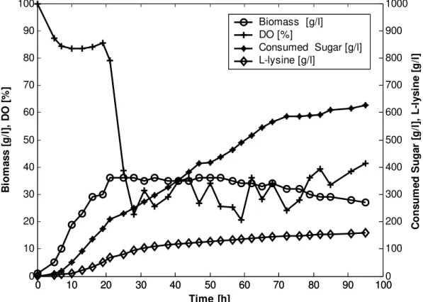
The fed-batch fermentation process with droppings is carried out at laboratory scale fermentor with 7 litres total volume. Corynebacterium sp. - B031 is used as a producer. The strain is dominantly characterised with prototrophic nature, which ensures successfully carrying out of fed-batch process with big number of droppings. Analytical methods used for the characterisation of the process are as follows: biomass is measured as dry cell mass [g/l]; sugar concentration – as reducible compounds [g/l]; L-lysine – by chromatographic method. During the process on-line measurement of differed physical-chemical variables are done by proper sensors. The experimental data are shown in Fig. 1. Dissolved oxygen tension [%] is denoted as DO in Fig. 1.

0 10 20 30 40 50 60 70 80 90 100

Time [h]

B

io

m

a

s

[

g

/l]

, D

O

[

%

]

0 10 20 30 40 50 60 70 80 90 1000 100 200 300 400 500 600 700 800 900 1000

C

ons

um

e

d S

uga

r [

g/

l]

,

L-ly

s

ine

[

g/

l]

Biomass [g/l] DO [%]

Consumed Sugar [g/l] L-lysine [g/l]

Fig. 1 Time course of the experimental data

Primary data processing

(3)

• Transformation of the different measurements units of the concentration to unit [g/l].

• Equalisation of the fed-batch process to the batch one.

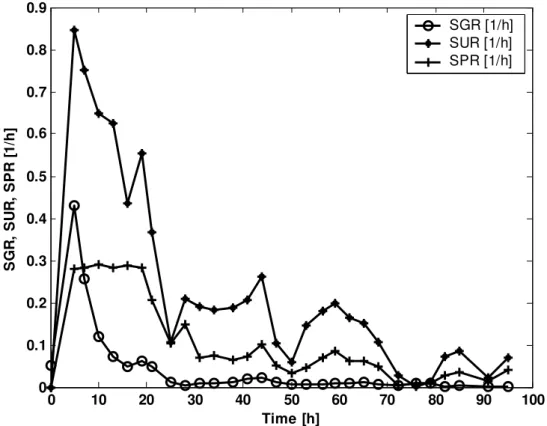
• Calculation of the specific rates: growth rate (µ), [h-1]; substrate utilisation rate, (ν) [h-1]; production rate (ρ), [h-1].

The specific rates are calculated by the equations:

µ=

T T

X X

, ν=

T C

X S

, ρ=

T T

X L

,

where:

XT – total biomass concentration expressed by [g/l];

SC – sugar consumed concentration, [g/l];

LT – total L-lysine concentration, [g/l];

C – dissolved oxygen tension, [%].

The calculated specific rates are shown in Fig. 2.

0 10 20 30 40 50 60 70 80 90 100

0 0.1 0.2 0.3 0.4 0.5 0.6 0.7 0.8 0.9

Time [h]

S

G

R

, SU

R

,

SPR

[

1

/h

]

SGR [1/h] SUR [1/h] SPR [1/h]

Fig. 2 The dynamic of the specific rates

SGR (instead of µ) – specific growth rate, SUR (instead of ν) – specific substrate utilization rate, SPR (instead of ρ) – specific production rate

Results and discussion

(4)

Generalised stoichiometric equations

Generalised stoichiometric equations present a possible reactions and stages of the discussed process. These equations present a hypothesis about specific mechanisms of the product formulation.

Suppose that the fermentation process could be described by the following system of generalised stoichiometric equations:

V V V L L X S C S S S X X S C X S OUT F OUT L OUT S OUT g X f 0 C C C R C C ⎯ ⎯ → ⎯ ⎯→ ⎯ ⎯ ⎯ → ⎯ ⎯→ ⎯ + + ⎯ ⎯ → ⎯ ⎯→ ⎯ ⎯ ⎯ → ⎯ ⎯→ ⎯ + ⎯→ ⎯ ϕ ϕ ϕ ϕ ϕ ϕ ϕ ϕ ϕ (1)

where: ϕX, ϕG, ϕS, ϕL, ϕF, ϕOUT are rates of the reactions, [g/l/h];

V0 - initial volume, [l];

Vf - final volume of the culture broth, [l];

X - biomass concentration, [g/l];

S - substrate concentration as a sugar remain concentration - SR or sugar consumed concentration – Sc, [g/l];

L - L-lysine concentration, [g/l];

C - dissolved oxygen tension, [%].

The rate ϕOUT takes into account the droppings of the culture broth.

Hypotheses about specific rates

The hypotheses concerning the specific rates of the amino acids biosynthesis are utilised as follows:

µ = µ(S, C),[h-1]

ν = ν(µ), [h-1];ν = ν(µ, X),[h-1] (2)

ρ = ρ(µ), [h-1];ρ=ρ(µ, X),[h-1].

It is assumed that at the discrete time moments

( )

t_k of the dropping the derivatives of the kinetics variables are equal to zero. Semi continuous or dropping conditions are obtained based on the material balance equation as follows:

• Dropping conditions for growth

( ) ( ) ( )

k k k IN

( )

k

OUT t µ t V t F t

F = − . (3)

• Dropping conditions for L-lysine production

( ) ( ) ( )

_{( ) ( )}

_k

( )

_k k

k k

k t t

t t t

t _IN

OUT V F

L X

ρ

(5)

• Dropping conditions for substrate utilization

( ) ( ) ( )

_{( ) ( )}

( )

( ) ( )

_{( )}

_⎟⎟ ⎠ ⎞ ⎜⎜ ⎝ ⎛ − + = k k k IN k IN k k k k k OUT t S t S t S t F t V t S t X t ν t

F (5)

Joint conditions are obtained by comparison of the above expressions. The comparison of the equations (3) and (4) yields

( ) ( ) ( )

_{( )}

k k k k t L t X t ρ t

µ = (6)

Following the same approach the comparing of the expressions (3) and (5) obtains the equality

( ) ( ) ( )

_{( )}

( )

_{( )}

( )

_⎟⎟ ⎠ ⎞ ⎜⎜ ⎝ ⎛ + ⎟⎟ ⎠ ⎞ ⎜⎜ ⎝ ⎛ = k k IN k k IN k k k k t S t S t V t F t S t X t ν t µ (7)

The final expression is derived based on equalities (6) and (7) as follows

( ) ( )

_{( ) ( )}

_{( )}

( )

_{( )}

( )

_{( )}

( )

_⎟⎟ ⎠ ⎞ ⎜⎜ ⎝ ⎛ + ⎟⎟ ⎠ ⎞ ⎜⎜ ⎝ ⎛ = k k k k k k k k k k t t t t t t t t t t S S V F S X ν L X

ρ IN IN

(8)

It could be emphasized that these conditions are satisfied at the discrete time moments

( )

t_k .

Identification procedure

The presented approach of the identification procedure includes the following stages:

• The linear regression or polynomial regressions are applied for selection of a preliminary structure of the models describing the specific rates and initial estimates of its parameters. The aim of this step is the selection of the appropriate model structure and the model fit to the experimental data. Experimental data transformations on this step are natural logarithm and an appropriate power of the exponential terms.

• The next step is done by a non-linear regression based on the selected model structure and initial values of the parameters without any transformations. These models are represented in the article. The model selection is done based on R2 coefficient model fit approximation and the results of the residual investigation.

• The final stage of identification is connected with the parametric optimisation of the models through the non-linear optimisation procedure under the confidence intervals of the parameters using Optimisation Toolbox. The Levenberg-Marquardt algorithm with least squares objective function is used for optimisation.

Models of the specific rates

After the identification procedure the specific growth rate is expressed as:

(

)

( )

(

)

(

)

(

a aS a S bC b C b S C

)

exp

(6)

The adequacy of the model (9) graphically presented in Fig. 3 is proved through the value of the determination coefficient R2 = 0,897692 obtained by the non-linear regression. The derived model is selected from the set of the models suitable for the experimental data subject to requirement for a minimal order of the polynomials in the model.

Table 1. Estimated parameters according to the model (9) with 95% confidence intervals

Parameters Estimate Asymptotic standard error

Lower limit Upper limit

a0 -10,7221 39,7702 - 92,804 71,3598

a1 0,00116321 0,107516 - 0,220739 0,223065

a2 0,0000174146 0,000101979 - 0,00019306 0,000227889

b1 34,1904 92,8428 - 157,428 225,809

b2 - 25,9271 81,0916 - 193,292 141,438

b3 - 0,0486574 0,11946 - 0,295211 0,197896

0 10 20 30 40 50 60 70 80 90 100

0 0.05 0.1 0.15 0.2 0.25 0.3 0.35 0.4 0.45

Time [h]

SG

R

[

1

/h

]

SGR [1/h] Model [1/h]

Fig. 3 Model approximation fit of the specific growth rate

Following the same approach the model of the specific utilization rate is obtained as:

( )

( ) ( )

( )

( ) ( )

(

)

(

c cµ c µ c µ c X c X c X c µ.X

)

exp

ν 7

3 6 2 5 4

3 3 2 2 1

0+ + + + + + +

= (10)

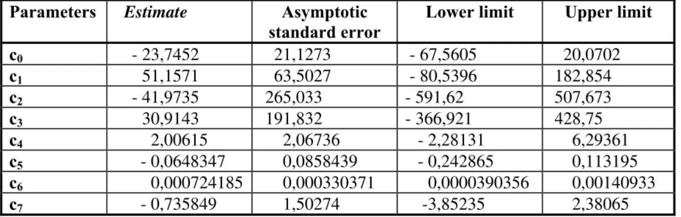
The value of the determination coefficient (R2 = 0,810537) proves the adequacy of this model (10).

(7)

Parameters Estimate Asymptotic

standard error

c0 - 23,7452 21,1273 - 67,5605 20,0702

c1 51,1571 63,5027 - 80,5396 182,854

c2 - 41,9735 265,033 - 591,62 507,673

c3 30,9143 191,832 - 366,921 428,75

c4 2,00615 2,06736 - 2,28131 6,29361

c5 - 0,0648347 0,0858439 - 0,242865 0,113195

c6 0,000724185 0,000330371 0,0000390356 0,00140933

c7 - 0,735849 1,50274 -3,85235 2,38065 The appropriate structure of the model and the estimates of the parameters are conformed by the plots in Fig. 4.

0 10 20 30 40 50 60 70 80 90 100

0 0.1 0.2 0.3 0.4 0.5 0.6 0.7 0.8 0.9

Time [h]

SU

R

[

1

/h

]

SUR [1/h] Model [1/h]

Fig. 4 Model approximation fit of the specific utilization rate

The important characterization of the L-lysine production is the specific production rate derived by the identification procedure as follows

( )

( ) ( )

(

)

(

) (

)

(

)

(

d dµ d µ d µ d X d X d X d µ.X

)

exp

ρ 7

3 6 2 5 4

3 3 2 2 1

0+ + + + + + +

= (11)

(8)

Parameters Estimate Asymptotic

standard error

d0 - 10,5439 28,4196 - 69,4828 48,3949

d1 51,4282 53,643 - 59,8209 162,677

d2 -127,521 289,047 - 726,969 471,928

d3 123,707 262,868 - 421,448 668,863

d4 0,36768 2,56514 - 4,95211 5,68747

d5 - 0,0017355 0,0705484 - 0,148044 0,144573

d6 - 0,000075946 0,00033325 - 0,000767066 0,000615174

d7 - 0,407434 1,3511 - 3,20945 2,39459 It could be seen that the model approximation fit describes the trend of the specific production rate (Fig. 5).

0 10 20 30 40 50 60 70 80 90 100

0 0.05 0.1 0.15 0.2 0.25 0.3 0.35

Time [h]

SP

R

[

1

/h

]

SPR [1/h] Model [1/h]

Fig. 5 Model approximation fit of the specific production rate

The obtained models with structure and estimates of the parameters are used on the next step of the synthesis of the model.

Unstructured dynamic mathematical model of the process

(9)

X V F X V F

µX K dt

dX IN OUT

1 − −

=

C OUT IN

IN C IN 2

C _S

V F S V F S V F

νX K dt

dS ₌ ₋ ₊ ₋

(12)

L V F L V F

ρX K dt

dL IN OUT

3 − −

=

OUT IN F

F dt dV

− =

where:

X – biomass concentration, [g/l];

L – L-lysine concentration, [g/l];

Sc – sugar consumed concentration, [g/l];

V – total volume of the culture broth, [l];

DLIN = FIN/V – dilution level, [h-1];

DLOUT = FOUT/V – dilution level of dropping, [h-1];

FIN – feeding rate, [l/h];

FOUT – dropping rate, [l/h].

The Levenberg-Marquardt algorithm with least squares objective function is used for parametric optimization.

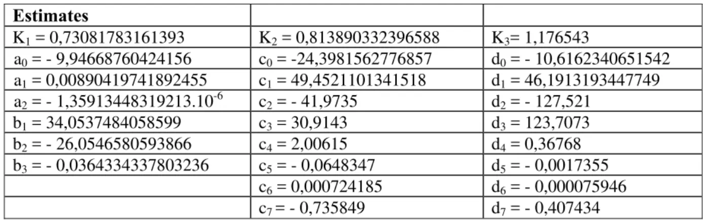
Table 4. Final estimation of the model parameters

Estimates

K1 = 0,73081783161393 K2 = 0,813890332396588 K3= 1,176543

a0 = - 9,94668760424156 c0 = -24,3981562776857 d0 = - 10,6162340651542

a1 = 0,00890419741892455 c1 = 49,4521101341518 d1 = 46,1913193447749

a2 = - 1,35913448319213.10-6 c2 = - 41,9735 d2 = - 127,521

b1 = 34,0537484058599 c3 = 30,9143 d3 = 123,7073

b2 = - 26,0546580593866 c4 = 2,00615 d4 = 0,36768

b3 = - 0,0364334337803236 c5 = - 0,0648347 d5 = - 0,0017355

c6 = 0,000724185 d6 = - 0,000075946

c7 = - 0,735849 d7 = - 0,407434

(10)

0 10 20 30 40 50 60 70 80 90 100 0

5 10 15 20 25 30 35 40

Time [h]

X, Xm

X [g/l]

Xm - Model [g/l]

Fig. 6 Time course of the biomass concentration

0 10 20 30 40 50 60 70 80 90 100

0 100 200 300 400 500 600 700

Time [h]

Sc

, S

m

Sc [g/l]

Sm - Model [g/l]

(11)

0 10 20 30 40 50 60 70 80 90 100 0

20 40 60 80 100 120 140 160 180

Time [h]

L,

Lm

L [g/l]

Lm - Model [g/l]

Fig. 8 Time course of the L-lysine production

0 10 20 30 40 50 60 70 80 90 100

2 2.2 2.4 2.6 2.8 3 3.2 3.4 3.6 3.8

Time [h]

V, Vm

V [g/l]

Vm - Model [g/l]

(12)

Conclusions

The following conclusions could be drown based on the results achieved so far:

1. The trend and values of the specific rates are estimated based on the experimental data and material balance followed by an additional data processing.

2. The linear regression or polynomial regressions are applied for selection of a preliminary structure of the models describing the specific rates and initial estimates of their parameters. The aim is the selection of the appropriate model structure and the model fit to the experimental data. The full regression analysis is done including the investigation of the residuals.

3. Non-linear regression, based on the selected model structure and initial values of the parameters, without any data transformations is applied as a next stage for mathematical model development. The model selection is done using R2 coefficient and the results of the residual investigation.

4. The final stage of the investigation is connected with the parametric optimization of the model through the non-linear optimization procedure under the confidence intervals of the parameters using Optimization Toolbox. The Levenberg-Maquardt algorithm with least squares objective function is used for optimization.

5. Based on the simulation results it could be concluded that the obtained mathematical model describes the trend of the experimental data in a satisfactory way.

References

1. Bastin G., L. Chen, V. Chotteau (1992). Can we Identify Biotechnological Processes?, Proceedings of IFAC, Modelling and Control of Biotechnological Processes, Colorado, USA, 83-88.

2. Georgiev Tz., Al. Ratkov, St. Tzonkov (1997). Mathematical Modelling of Fed-batch Fermentation Processes for Amino Acid Production, Mathematics and Computers in Simulation, 44, 171-285.

3. Georgiev Tz., Al. Ratkov, St. Tzonkov(1995). An Approach for Mathematical Modelling of Fed-batch Process for L-lysine Production, Biotechnology and Biotechnological equipment, 4, 84-92.

4. Leuchtenberger W., K. Huthmacher, K. Drauz (2005). Biotechnological Production of Amino Acids and Derivatives: Current Status and Prospects, Appl. Microbiol. Biotechnol., 69, 1-8.

5. MathWorks Inc. (2003). MATLAB User's Guide.

6. MathWorks Inc. (2003). System Identification Toolbox, User's Guide. 7. MathWorks Inc. (2003). SIMULINK, Using SIMULINK.

8. MathWorks Inc. (2003). Optimization Toolbox, User’s Guide.