NHESSD
1, 7333–7356, 2013Storm-surge prediction at the
Tanshui estuary
C.-P. Tsai et al.
Title Page
Abstract Introduction
Conclusions References
Tables Figures
◭ ◮
◭ ◮
Back Close
Full Screen / Esc
Printer-friendly Version Interactive Discussion
Discussion
P
a
per
|
D
iscussion
P
a
per
|
Discussion
P
a
per
|
Discuss
ion
P
a
per
Nat. Hazards Earth Syst. Sci. Discuss., 1, 7333–7356, 2013 www.nat-hazards-earth-syst-sci-discuss.net/1/7333/2013/ doi:10.5194/nhessd-1-7333-2013
© Author(s) 2013. CC Attribution 3.0 License.
Natural Hazards and Earth System Sciences
Open Access
Discussions
This discussion paper is/has been under review for the journal Natural Hazards and Earth System Sciences (NHESS). Please refer to the corresponding final paper in NHESS if available.
Storm-surge prediction at the Tanshui
estuary: development model for maximum
storm surges
C.-P. Tsai1, C.-Y. You1, and C.-Y. Chen2
1
Department of Civil Engineering, National Chung Hsing University, Kuo Kuang Rd., Taichung 402, Taiwan
2
Department and Graduate School of Computer Science, National Pingtung University of Education, No. 4–18, Ming Shen Rd., Pingtung 90003, Taiwan
Received: 16 October 2013 – Accepted: 13 November 2013 – Published: 10 December 2013 Correspondence to: C.-Y. Chen ([email protected])
NHESSD
1, 7333–7356, 2013Storm-surge prediction at the
Tanshui estuary
C.-P. Tsai et al.
Title Page
Abstract Introduction
Conclusions References
Tables Figures
◭ ◮
◭ ◮
Back Close
Full Screen / Esc
Printer-friendly Version Interactive Discussion
Discussion
P
a
per
|
D
iscussion
P
a
per
|
Discussion
P
a
per
|
Discuss
ion
P
a
per
|
Abstract
This study applies artificial networks, including both the supervised multilayer percep-tion neural network and the radial basis funcpercep-tion neural network to the predicpercep-tion of storm-surges at the Tanshui estuary in Taiwan. The optimum parameters for the pre-diction of the maximum storm-surges based on 22 previous sets of data are discussed.
5
Two different neural network methods are adopted to build models for the prediction of storm surges and the importance of each factor is also discussed. The factors relevant to the maximum storm surges, including the pressure difference, maximum wind speed and wind direction at the Tanshui Estuary and the flow rate at the upstream station, are all investigated. These good results can further be applied to build a neural network
10
model for prediction of storm surges with time series data.
1 Introduction
Storm surges are sudden rises of water levels that can occur during typhoons, lead-ing to the risk of floodlead-ing in low-lylead-ing coastal areas. Generally, storm surges are pre-dicted using numerical methods. For example, Kawahara et al. (1980), Westerink et
15
al. (1992), Blainetal (1994), and Hsu et al. (1999) applied the finite element method, Yen and Chou (1979), Walton and Christensen (1980), Harper and Sobey (1983), and Hwang and Yao (1987) applied the finite difference method with nonlinear shallow water equations to simulate storm surges.
In recent years, neural network technology has become more and more mature. It
20
has been widely applied to non-linear natural phenomena. For example, Grubert (1995) used feed-forward back-propagation neural networks to predict the flow rate at a river mouth. Deo and Naidu (1999) used neural networks to build a model for real-time wave prediction. The results show that these neural networks perform better than that of the AR model for wave prediction. Tsai and Lee (1999) used back-propagation neural
net-25
works for real-time tide prediction. The predictions were very accurate and parameter
NHESSD
1, 7333–7356, 2013Storm-surge prediction at the
Tanshui estuary
C.-P. Tsai et al.
Title Page
Abstract Introduction
Conclusions References
Tables Figures
◭ ◮
◭ ◮
Back Close
Full Screen / Esc
Printer-friendly Version Interactive Discussion
Discussion
P
a
per
|
D
iscussion
P
a
per
|
Discussion
P
a
per
|
Discuss
ion
P
a
per
fitting was not required for that model. Tsai et al. (2002) used the neural network tech-nique for forecasting and supplementing the time series of wave data using neighbor station wave records. Marzenna (2003) used neural networks to predict storm surges and compared the results obtained using different neural network topologies. Lee et al. (2004) used short-term observational data to predict long-term sea levels with a
5
back-propagation neural network and obtained accurate results.
Tsai et al. (2005) used back-propagation neural networks for the training of a wa-ter level time series model with data from previous typhoons used as training data to predict later typhoons. The prediction results were very good. However, the model was only used to predict overall water levels during storms. Storm surge values obtained
10
by deducting astronomical tides from the predicted overall water levels might not be the same as actual values. In practice, astronomical tides plus storm surges equal the overall water levels during storms. Currently, astronomical tides can be well predicted using the harmonic analysis method or other numerical methods. Moreover, the max-imum storm surge plus the highest spring tide may provide the potential for coastal
15
inundation. Thus, the focus of this study is on the maximum storm surges.
2 Mathematical formulations
2.1 Storm surge empirical formula
Storm surges are also called irregular weather water levels. Studies on storm surges at specific spots are more meaningful with higher practical values. Storm surges are
20
also related to weather conditions (e.g., wind speed, wind direction, and minimum at-mospheric pressure). Regarding maximum storm surge estimations, Cornner (1957) believed that a larger center of low pressure would lead to higher wind speeds at a station. The pressure can be used to estimate storm surges. Unoki and Isozaki (1966) also believed that maximum storm surges can be expressed in terms of pressure. They
NHESSD
1, 7333–7356, 2013Storm-surge prediction at the
Tanshui estuary
C.-P. Tsai et al.
Title Page
Abstract Introduction
Conclusions References
Tables Figures
◭ ◮
◭ ◮
Back Close
Full Screen / Esc
Printer-friendly Version Interactive Discussion
Discussion
P
a
per
|
D
iscussion
P
a
per
|
Discussion
P
a
per
|
Discuss
ion
P
a
per
|
analyzed all the storm surge data in Japan to obtain an empirical formulation for pre-dicting storm surges at estuaries by the open sea.
Horikawa (1978) referenced the analysis results of previous actual data from Japan and suggested that, in addition to pressure, other parameters such as wind speed should also be taken into consideration. Their empirical formula is as follows:
5
ζmax=A∆P +B(Vmax)2cosθ, (1)
whereζmaxis the maximum storm surge,∆P is the maximum pressure difference dur-ing the storm surge,Vmaxis the maximum wind speed during the typhoon,θis the angle between the direction of the wind with the maximum wind speed and the tide-gauge station’s normal line, andAand B are the empirical constants at the maximum storm
10
surge.
2.2 Multi layer perception network
A multi layer perception (MLP) network is a supervised learning method. This type of topology contains one input layer, one or more hidden layers, and one output layer. Data is sent to the output layer from the input layer using the feedforward method. The
15
formulas are listed below:
yj =f netj
, (2)
netj = X
i
W
i jXi−Bj, (3)
whereyj is the output variable,Wi j is the weight between thejth neural layer and the
20
ith neural layer,Xi is the input variable as a biomimetic neuron input signal, f(netj) is the transformation function as a biomimetic non-linear function of the neurons,Bj is
NHESSD
1, 7333–7356, 2013Storm-surge prediction at the
Tanshui estuary
C.-P. Tsai et al.
Title Page
Abstract Introduction
Conclusions References
Tables Figures
◭ ◮
◭ ◮
Back Close
Full Screen / Esc
Printer-friendly Version Interactive Discussion
Discussion
P
a
per
|
D
iscussion
P
a
per
|
Discussion
P
a
per
|
Discuss
ion
P
a
per
the threshold (bias) for thejth neuron, and netj is the consolidation function for thejth neuron.
A transformation function is usually an S curve called a sigmoid function which in-creases stability and can be written as:
yj =fXWi jXi−Bj= 1
1+e−(PWi jXi−Bj)
. (4)
5
The MLP network learning method, like the back-propagation neural network, is based on iteration. However, it allows for more than one hidden layer, therefore it can handle rather complex functions. Furthermore, with optimized network algorithms, the time and number of iterations required can be reduced. Usually the number of layers and neurons are obtained using a trial and error method. The best topology can thus
10
be found. With enough hidden layers and neurons, any continuous function can be approximated.
2.3 Radial basis function network
The topology of the radial basis function (RBF) network is similar to that of the MLP net-work. Basically, the most advantageous feature of the RBF network is its fast learning
15
speed, making it suitable for application in real-time systems. Its output can be written as:
Fx′=
N X
j=1
wjφjx′+Bj, (5)
wherex′ is the input vector (x
1,. . ., xp) T
, Wj is the weight from the jth layer to the output layer,Bj is the threshold (bias) for thejth neuron,ψj is the basis function of the
20
NHESSD
1, 7333–7356, 2013Storm-surge prediction at the
Tanshui estuary
C.-P. Tsai et al.
Title Page Abstract Introduction Conclusions References Tables Figures ◭ ◮ ◭ ◮ Back Close
Full Screen / Esc
Printer-friendly Version Interactive Discussion Discussion P a per | D iscussion P a per | Discussion P a per | Discuss ion P a per |
A common basis function used for the RBF network is a Gaussian function, which can be written as:
φj(x′)=exp −
x′−Uj
2
2σj2
,j=1, 2, 3. . . N, (6)
whereσj is the smoothing parameter (called the width in this study) of thejth neuron which controls the radial basis function,Uj is the center of the neurons in thejth radial
5
basis function hidden layer, and x
′
−Uj
is the Euclidean distance between Uj and the input vector.
3 Maximum storm surge prediction model
According to Murty (1984), over the past century, an average of 3.5 typhoons has struck Taiwan per year. Storm surges are very likely to occur at estuaries in the northern areas
10
of Taiwan, such as Tanshui which is bordered by the Taiwan Strait. Data from the station at the Tanshui Estuary were collected in order to explore these storm surges.
3.1 Data sources
This study used storm surge and weather data acquired during typhoons from the station at the Tanshui Estuary (the tide-gauge station outside the southern dock of the
15
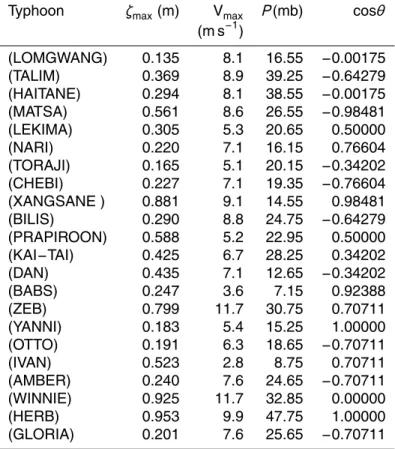
second fishing port by the Tanshui Estuary) from 1996–2001 and in 2005. Data for 22 typhoons were selected based on their paths and whether they had caused serious storm surges at the Tanshui Estuary. The data used are summarized in Table 1. Data from the Xiulang Station, a hydrological station 25 km downstream from the Tanshui Estuary operated the Water Resources Agency on the Tamsui River were used.
20
NHESSD
1, 7333–7356, 2013Storm-surge prediction at the
Tanshui estuary
C.-P. Tsai et al.
Title Page
Abstract Introduction
Conclusions References
Tables Figures
◭ ◮
◭ ◮
Back Close
Full Screen / Esc
Printer-friendly Version Interactive Discussion
Discussion
P
a
per
|
D
iscussion
P
a
per
|
Discussion
P
a
per
|
Discuss
ion
P
a
per
3.2 Pre-processing of data and evaluation indexes
Before training a neural network, pre-processing of the input data is very important. Input data must be normalized as discussed below:
xnew=
Dmin+ xold−xmin
xmax−xmin ×(Dmax−Dmin)
, (7)
where Dmin and Dmax represent the range of linear mapping, xmax and xmin are the
5
maximum and minimum values in the series, andxoldand xnew are the series before and after transformation.
Generally, network performances can be efficiently shown by looking at the errors and correlations obtained using two separate statistical indexes, the root mean square errors (RMSE) and correlation coefficients (C.C.). Their definitions follow:
10
RMSE= v u u u t
n P
k=1
(yk−yˆk)2
n , (8)
wherenis the sample size,yk is the observed value of thekth sample point, and ˆykis thekth estimation.
C.C.= n P
k=1
(yk−y¯k)y¯ˆk−y¯k s
n P
k=1
(yk−y¯k)2 Pn k=1
¯ˆ
yk−y¯k
2
, (9)
whereyk is the observed value of thekth sample point, ˆyk is thekth estimation, ¯ˆyk is
15
NHESSD
1, 7333–7356, 2013Storm-surge prediction at the
Tanshui estuary
C.-P. Tsai et al.
Title Page
Abstract Introduction
Conclusions References
Tables Figures
◭ ◮
◭ ◮
Back Close
Full Screen / Esc
Printer-friendly Version Interactive Discussion
Discussion
P
a
per
|
D
iscussion
P
a
per
|
Discussion
P
a
per
|
Discuss
ion
P
a
per
|
3.3 Topology presentation of neural networks
In this study, the topologies of neural networks are presented in the form of “IxHyOz”, whereIx represents the number of neurons (factors which influenced storm surges, such as pressure difference, wind speed, etc.) in the input layer,Hyrepresents the num-ber of hidden layers, andOzrepresents the number of output variables. The number of
5
output neurons was 1 (z=1) because there was only one variable to be predicted, the storm surge.
3.4 Empirical formulation
To obtain the empirical formula for finding the maximum storm surge, the generalized least squares method was applied with data for the 22 selected typhoons being used
10
for the regression analysis. The following empirical constants for the Tanshui Estuary were obtained:A=0.00952 andB=0.0031. The formula can be written as:
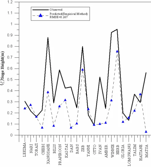
ζmax=0.00952∆P+0.0031(Vmax)2cosθ. (10)
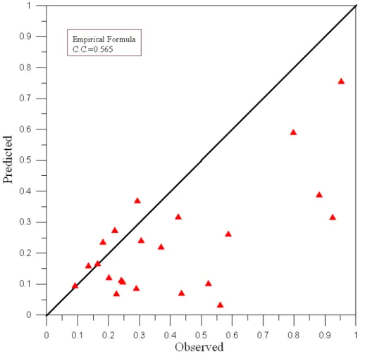
Equation (10) is applied to the data for the 22 typhoons and the results are summa-rized in Fig. 1. According to the graph, the estimations obtained with the storm surge
15
empirical formula are mostly lower than the observed values. The reason could be that there was not enough data for empirical calculation of the storm surge, leading to poor precision. The correlation coefficient is 0.565, as shown in Fig. 2.
4 Empirical verification
Three models were used for discussion based on the pressure difference (∆P), the
20
wind field factor (U =Vmax2 cosθ) at the Tanshui Estuary and the flow rate (Q) from the upstream Xiulang Station (make segmentation). Model A:ζmax=f (∆P)
Model B:ζmax=f (∆P,U) Model C:ζmax=f (∆P,U,Q)
NHESSD
1, 7333–7356, 2013Storm-surge prediction at the
Tanshui estuary
C.-P. Tsai et al.
Title Page
Abstract Introduction
Conclusions References
Tables Figures
◭ ◮
◭ ◮
Back Close
Full Screen / Esc
Printer-friendly Version Interactive Discussion
Discussion
P
a
per
|
D
iscussion
P
a
per
|
Discussion
P
a
per
|
Discuss
ion
P
a
per
4.1 MODEL A
In line with scholars such as Cornner et al. (1957) and Isozaki (1966) who believe that pressure differences can be used to estimate maximum storm surges, this study first utilizes the pressure difference as the only input variable to build a neural network model to predict the maximum storm surge. As can be seen in Table 2, in Model A, the
5
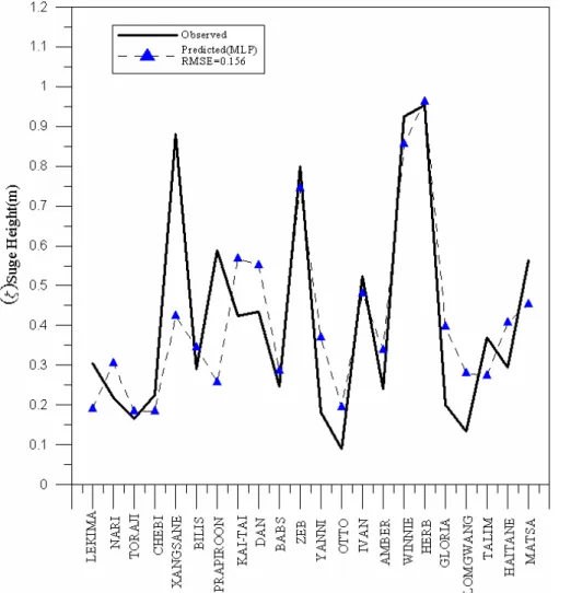
best topologies for the MLP and RBF neural network models areI1H7O1 and I1H8O1, respectively. According to the storm surge predictions shown in Figs. 3 and 4, the MLP model could predict some of the maximum storm surges based on a single input variable.
According to Table 2, although there was not sufficient precision, when using the
10
pressure difference as the only input variable, the performance of the neural network model was better than that of the empirical formula.
4.2 MODEL B
In Model A, the only input variable was the maximum pressure difference. Then after that, another input variable, the corresponding wind field factor, was added to predict
15
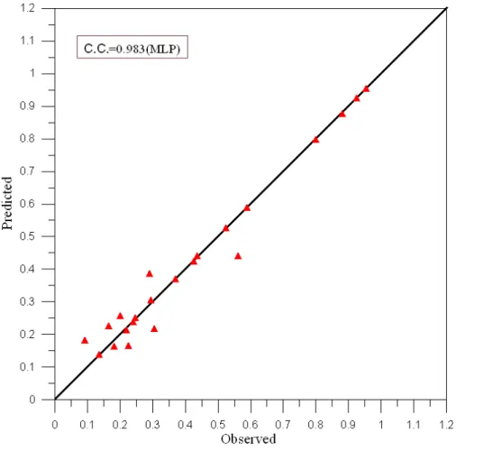
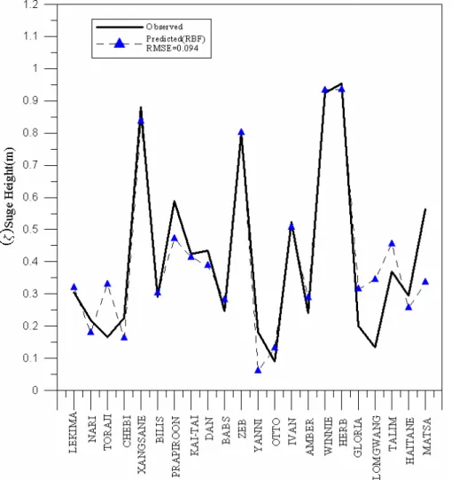
maximum storm surges. According to Table 2, the best network topologies for the MLP and RBF neural network models wereI2H7O1andI2H11O1. According to the correlation coefficients in Figs. 5 and 6, the predictions for maximum storm surges in Model B, in which the maximum wind factor was considered, were better than those in Model A. The correlation coefficient for the MLP model was 0.983, and that of the RBF model
20
was 0.935.
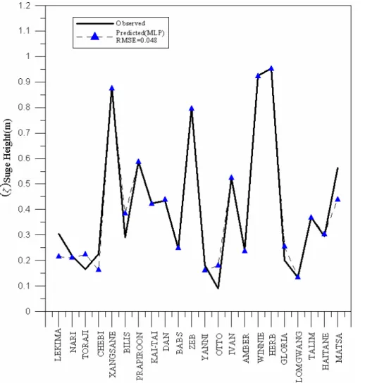
Figures 3, 4, 7, and 8 show the maximum storm surge predictions of Models A and B. According to these figures, the predictions obtained using both the MLP model and the RBF model in Model B were more precise than those in Model A. It is also found that the MLP predictions were more precise for typhoons causing larger storm surges. They
25
NHESSD
1, 7333–7356, 2013Storm-surge prediction at the
Tanshui estuary
C.-P. Tsai et al.
Title Page
Abstract Introduction
Conclusions References
Tables Figures
◭ ◮
◭ ◮
Back Close
Full Screen / Esc
Printer-friendly Version Interactive Discussion
Discussion
P
a
per
|
D
iscussion
P
a
per
|
Discussion
P
a
per
|
Discuss
ion
P
a
per
|
is obvious that the influence of wind factor should not be ignored in the prediction of the maximum storm surge, especially for typhoons causing larger storm surges.
4.3 MODEL C – influences of upstream flow
The storm surges in estuaries can be categorized into those in estuaries near seas and in estuaries near rivers. The storm surges discussed in this study are the former.
5
The maximum pressure difference and wind factor were used as inputs in Model B. In addition to the maximum pressure difference and the corresponding maximum wind speed, the upstream flow was input as well in Model C. According to Table 2, the best topologies for the MLP and RBF neural network models were I3H6O1 and I3H10O1,
respectively.
10
According to the correlation coefficients in Table 2, the MLP and RBF models per-formed better for Model C (with upstream flow being input) than for Model B (without the input of upstream flow). However, the correlation for the MLP model in Model C were only 0.003 higher than that in Model B, while the correlation for the RBF model in Model C was lower than those in Model B.
15
Although according to the predictions of storm surges as shown in Figs. 7 and 9, the RMSE for the MLP model in Model B was slightly higher than that in Model C, while it can be seen from Figs. 8 and 10 that the RMSE for the RBF model was slightly lower for Model B than for Model C. Thus, it is likely that although the upstream flow had some influence on storm surge, the influence is far smaller than that of wind field and
20
low pressure.
5 Conclusions
According to the results of Models A, B, and C, if the pressure difference was the sole input, Model A might be too dependent on one single factor to obtain precise predictions. In Model B, the factors used in Horikawa’s (1978) formula were adopted,
25
NHESSD
1, 7333–7356, 2013Storm-surge prediction at the
Tanshui estuary
C.-P. Tsai et al.
Title Page
Abstract Introduction
Conclusions References
Tables Figures
◭ ◮
◭ ◮
Back Close
Full Screen / Esc
Printer-friendly Version Interactive Discussion
Discussion
P
a
per
|
D
iscussion
P
a
per
|
Discussion
P
a
per
|
Discuss
ion
P
a
per
where the wind field and maximum pressure difference were input. Neural network models can be used to predict highly non-linear influences, thereby improving on the disadvantages of the empirical formula. In Model C, although the upstream flow was a factor of influence on the storm surges, manual observations are required to obtain flow information during typhoons. However, it is very common for there to be missing
5
values or large observation errors. Based on the above review and discussion, the best input factors for Model B would further be applied to build a neural network prediction of storm surges with time series.
Acknowledgements. The authors are appreciative of the support to the CYC and CPT received
from the National Science Council of the Republic of China, under Grant No. NSC
99-2628-10
E-153-001 and No. NSC 96-2221-E-005-077-MY3. They are also most grateful for the kind assistance of the editor and for the constructive suggestions from the anonymous reviewers, all of which have led to the making of several corrections and have greatly aided us to improve the presentation of this paper.
References 15
Blain, C. A., Westerink, J. J., and Luettich, R. A., Jr.: The influence of domain size on the response characteristics of a hurricane storm surge model, J. Geophysical Res., 99, 18467– 18479, 1994.
Conner, W. C., Kraft, R. H., and Lee, H. D.: Empirical methods for forecasting the maximum storm tide due to hurricanes and other tropical storms, Monthly Weather Review, 85, 113–
20
116, 1957.
Deo, M. C. and Sridhar, N. C.: Real time wave forecasting using neural networks, Ocean Eng., 26, 191–203, 1999.
Grubert, J. P.: Prediction of estuarine instabilities with artificial neural networks, J. Comput. Civil Eng., 9, 266–274, 1995.
25
Harper, B. A. and Sobey, R. J.: Open-boundary conditions for open-coast hurricane storm surge, Coast. Eng. Japan, 7, 41–60, 1983.
NHESSD
1, 7333–7356, 2013Storm-surge prediction at the
Tanshui estuary
C.-P. Tsai et al.
Title Page
Abstract Introduction
Conclusions References
Tables Figures
◭ ◮
◭ ◮
Back Close
Full Screen / Esc
Printer-friendly Version Interactive Discussion
Discussion
P
a
per
|
D
iscussion
P
a
per
|
Discussion
P
a
per
|
Discuss
ion
P
a
per
|
Hsu, T. W., Liao, J. M. and Lee, Z. S.: Prediction of storm surge at northestern coast of Taiwan by finite element method, J. Chinese Institute of Civil and Hydraulic Eng., 11, 849–857, 1999. Hwang, R. R. and Yao, C. C.: A semi-implicit numerical model for storm surges, J. Chinese
Instit. Engin., 10, 463–472, 1987.
Kawahara, M., Nakazawa, S., Ohmori, S., and Tagaki, T.: Two-step explicit finite element
5
method for storm surge propagation analysis, Int. J. for Numerical Methods Eng., 15, 1129– 1148, 1980.
Lee, T. L.: Back-propagation neural network for long-term tidal predictions, Ocean Eng., 31, 225–238, 2004.
Marzenna, S.: Forecast of storm surge by means of artificial neural network, J. Sea Res., 49,
10
317–322, 2003.
Murty, T. S.: Storm surges: Meteorological ocean tides, Canadian Bulletin of Fisheries and Aquatic Science (212), Dept. Fisheries Oc. Canada, 1984.
Tsai, C. P. and Lee, T. L.: Back-propagation neural network in tidal-level forecasting, J. Water-way, Port, Coastal and Ocean Eng., ASCE125, 195–202, 1999.
15
Tsai, C. P., Lin, C., and Shen, J. N.: Neural network for wave forecasting among multi-stations, Ocean Eng., 29, 1683–1695, 2002.
Tsai, C. P., Lee, T. L., Yang, T. J., and Hsu, Y. J.: Back-propagation neural networks for predic-tion of storm surge, Proceedings of the Eighth Internapredic-tional Conference on the Applicapredic-tion of Artificial Intelligence to Civil, Structural and Environmental Eng., Paper (45), Civil-comp
20
Press, UK, 2005.
Unoki, S. and Isozaki, I.: A possibility of generation of surf beat, Proceedings of the 10th Inter-national Conference on Coastal Eng., ASCE, 1, 1207–1216, 1966.
Walton, R. and Christensen, B. A.: Friction factors in storm surges over inland areas, J. Water-way, Port, Coastal and Ocean Division, ASCE106, 261–271, 1980.
25
Westerink, J. J., Luettich, R. A., Baptista, A. M.,Scheffner, N. W., and Farrar, P.: Tide and storm surge predictions using a finite element model, J. Hrdraulic Eng., ASCE118, 1373–1390, 1992.
Yen, G. T. and Chou, F. K.: Moving boundary numerical surge model, J. Waterway, Port, Coastal and Ocean Division, ASCE105, 247–263, 1979.
30
NHESSD
1, 7333–7356, 2013Storm-surge prediction at the
Tanshui estuary
C.-P. Tsai et al.
Title Page
Abstract Introduction
Conclusions References
Tables Figures
◭ ◮
◭ ◮
Back Close
Full Screen / Esc
Printer-friendly Version Interactive Discussion
Discussion
P
a
per
|
D
iscussion
P
a
per
|
Discussion
P
a
per
|
Discuss
ion
P
a
per
Table 1.Maximum storm surge data.
Typhoon ζmax(m) Vmax P(mb) cosθ
(m s−1)
(LOMGWANG) 0.135 8.1 16.55 −0.00175
(TALIM) 0.369 8.9 39.25 −0.64279
(HAITANE) 0.294 8.1 38.55 −0.00175
(MATSA) 0.561 8.6 26.55 −0.98481
(LEKIMA) 0.305 5.3 20.65 0.50000 (NARI) 0.220 7.1 16.15 0.76604 (TORAJI) 0.165 5.1 20.15 −0.34202
(CHEBI) 0.227 7.1 19.35 −0.76604
(XANGSANE ) 0.881 9.1 14.55 0.98481 (BILIS) 0.290 8.8 24.75 −0.64279
(PRAPIROON) 0.588 5.2 22.95 0.50000 (KAI−TAI) 0.425 6.7 28.25 0.34202
(DAN) 0.435 7.1 12.65 −0.34202
(BABS) 0.247 3.6 7.15 0.92388 (ZEB) 0.799 11.7 30.75 0.70711 (YANNI) 0.183 5.4 15.25 1.00000 (OTTO) 0.191 6.3 18.65 −0.70711
(IVAN) 0.523 2.8 8.75 0.70711 (AMBER) 0.240 7.6 24.65 −0.70711
NHESSD
1, 7333–7356, 2013Storm-surge prediction at the
Tanshui estuary
C.-P. Tsai et al.
Title Page
Abstract Introduction
Conclusions References
Tables Figures
◭ ◮
◭ ◮
Back Close
Full Screen / Esc
Printer-friendly Version Interactive Discussion
Discussion
P
a
per
|
D
iscussion
P
a
per
|
Discussion
P
a
per
|
Discuss
ion
P
a
per
|
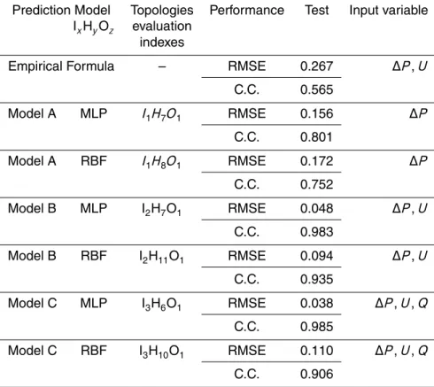
Table 2.Comparison of models for the prediction of storm surges.
Prediction Model Topologies Performance Test Input variable IxHyOz evaluation
indexes
Empirical Formula – RMSE 0.267 ∆P,U
C.C. 0.565
Model A MLP I1H7O1 RMSE 0.156 ∆P
C.C. 0.801
Model A RBF I1H8O1 RMSE 0.172 ∆P
C.C. 0.752
Model B MLP I2H7O1 RMSE 0.048 ∆P,U
C.C. 0.983
Model B RBF I2H11O1 RMSE 0.094 ∆P,U
C.C. 0.935
Model C MLP I3H6O1 RMSE 0.038 ∆P,U,Q
C.C. 0.985
Model C RBF I3H10O1 RMSE 0.110 ∆P,U,Q
C.C. 0.906
NHESSD
1, 7333–7356, 2013Storm-surge prediction at the
Tanshui estuary
C.-P. Tsai et al.
Title Page
Abstract Introduction
Conclusions References
Tables Figures
◭ ◮
◭ ◮
Back Close
Full Screen / Esc
Printer-friendly Version Interactive Discussion
Discussion
P
a
per
|
D
iscussion
P
a
per
|
Discussion
P
a
per
|
Discuss
ion
P
a
per
|
Fig. 2.Correlation coefficients from the storm surge empirical formula.
NHESSD
1, 7333–7356, 2013Storm-surge prediction at the
Tanshui estuary
C.-P. Tsai et al.
Title Page
Abstract Introduction
Conclusions References
Tables Figures
◭ ◮
◭ ◮
Back Close
Full Screen / Esc
Printer-friendly Version Interactive Discussion
Discussion
P
a
per
|
D
iscussion
P
a
per
|
Discussion
P
a
per
|
Discuss
ion
P
a
per
|
Fig. 4.RBF predictions of maximum storm surges (Model A).
NHESSD
1, 7333–7356, 2013Storm-surge prediction at the
Tanshui estuary
C.-P. Tsai et al.
Title Page
Abstract Introduction
Conclusions References
Tables Figures
◭ ◮
◭ ◮
Back Close
Full Screen / Esc
Printer-friendly Version Interactive Discussion
Discussion
P
a
per
|
D
iscussion
P
a
per
|
Discussion
P
a
per
|
Discuss
ion
P
a
per
|
Fig. 6. Correlation coefficients of the RBF maximum storm surge predictions and observed values (Model B).
NHESSD
1, 7333–7356, 2013Storm-surge prediction at the
Tanshui estuary
C.-P. Tsai et al.
Title Page
Abstract Introduction
Conclusions References
Tables Figures
◭ ◮
◭ ◮
Back Close
Full Screen / Esc
Printer-friendly Version Interactive Discussion
Discussion
P
a
per
|
D
iscussion
P
a
per
|
Discussion
P
a
per
|
Discuss
ion
P
a
per
|
Fig. 8.Predictions of maximum storm surge using the RBF model (Model B).
NHESSD
1, 7333–7356, 2013Storm-surge prediction at the
Tanshui estuary
C.-P. Tsai et al.
Title Page
Abstract Introduction
Conclusions References
Tables Figures
◭ ◮
◭ ◮
Back Close
Full Screen / Esc
Printer-friendly Version Interactive Discussion
Discussion
P
a
per
|
D
iscussion
P
a
per
|
Discussion
P
a
per
|
Discuss
ion
P
a
per
|
Fig. 10.Predictions of maximum storm surge using the RBF model (Model C).