Comparing model performance of two rainfall-runoff models in the Rhine basin using different atmospheric forcing data sets

(1)

HESSD

4, 4325–4360, 2007

Comparing model performance in the

Rhine basin

A. H. te Linde et al.

Title Page

Abstract Introduction

Conclusions References

Tables Figures

◭ ◮

Back Close

Full Screen / Esc

Printer-friendly Version

Interactive Discussion

EGU

Hydrol. Earth Syst. Sci. Discuss., 4, 4325–4360, 2007 www.hydrol-earth-syst-sci-discuss.net/4/4325/2007/ © Author(s) 2007. This work is licensed

under a Creative Commons License.

Hydrology and Earth System Sciences Discussions

Papers published inHydrology and Earth System Sciences Discussionsare under open-access review for the journalHydrology and Earth System Sciences

Comparing model performance of two

rainfall-runo

_ff

models in the Rhine basin

using di

_ff

erent atmospheric forcing data

sets

A. H. te Linde1, J. C. J. H. Aerts1, R. T. W. L. Hurkmans2, and M. Eberle3 1

Institute for Environmental Studies (IVM), Faculty of Earth and Life Sciences, Vrije Universiteit, De Boelelaan 1087, 1081 HV Amsterdam, The Netherlands

2

Hydrology and Quantitative Water Management, Wageningen University, Wageningen, The Netherlands

3

Federal Institute of Hydrology (BfG), Koblenz, Germany

Received: 16 November 2007 – Accepted: 16 November 2007 – Published: 4 December 2007

(2)

HESSD

4, 4325–4360, 2007

Rhine basin

Title Page

Tables Figures

◭ ◮

Back Close

Full Screen / Esc

Interactive Discussion Abstract

Due to the growing wish and necessity to simulate the possible e_ffects of climate change on the discharge regime on large rivers such as the Rhine in Europe, there is a need for well performing hydrological models that can be applied in climate change scenario studies. There exists large variety in available models and there is an ongoing 5

debate in research on rainfall-runoffmodelling on whether or not physically based dis-tributed models better represent observed discharges than conceptual lumped model approaches do. In this paper, the hydrological models HBV and VIC were compared for the Rhine basin by testing their performance in simulating discharge. Overall, the semi-distributed conceptual HBV model performed much better than the distributed 10

physically based VIC model (E₌0.62, r2₌0.65 vs. E₌0.31, r2₌0.54 at Lobith). It is argued here that even for a well-documented river basin such as the Rhine, more com-plex modelling does not automatically lead to better results. Moreover, it is concluded that meteorological forcing data has a considerable influence on model performance, irrespectively to the type of model structure and the need for ground-based meteoro-15

logical measurements is emphasized.

1 Introduction

It is expected that climate change will have major implications for the discharge regime of many rivers around the world (Kundzewicz et al., 2007). Changes in seasonal dis-charge are projected for river basins in mid-latitude regions, such as the Rhine basin 20

in Europe. Seasonal discharge will most likely shift to more discharge in winter and less discharge in summer, and the frequencies of floods and droughts are expected to increase (Buishand and Lenderink, 2004; Kwadijk, 1993; Middelkoop et al., 2001). Recent climate change research focuses on simulating changes in the magnitude and frequencies of flood events using different models that are either developed for sce-25

(3)

HESSD

4, 4325–4360, 2007

Rhine basin

Title Page

Tables Figures

◭ ◮

Back Close

Full Screen / Esc

EGU

Our understanding of the discharge generating processes in the Rhine basin, though, is still deficient and modelling results for describing the current hydrological situation at basin scale are of moderate quality. For instance, extreme events inside the cali-brated range are both over and underestimated and it is difficult to separate the effects of errors in input data and model structure (Weerts, 2003). This increases the inherent 5

uncertainty when using models outside their calibrated range, as is common practice in climate scenarios studies. Thus there is a need for a well performing hydrological model on extreme events that can be applied in various climate scenario studies, but there exists large variety in available models. Since these issues are common in ap-plications of hydrological modelling in other regions as well, we chose to compare two 10

rainfall-runo_ffmodels for the Rhine basin with diverge model structures.

The semi-distributed conceptual model HBV (Hydrologiska Byrans Vattenbal-ansavdelning) (Bergstr ¨om, 1976; Lindstr ¨om et al., 1997) has been applied in multiple studies for the Rhine basin since 1999 by both the German Federal Institute of Hy-drology and the Dutch Ministry of Transport, Public Works and Water Management 15

(M ¨ulders et al., 1999; Weerts and Van der Klis, 2004; Eberle et al., 2005). However, the HBV model does not exactly describe all the physical processes that are believed to be of major importance for the simulation of timing and magnitude of extreme flood and drought events (Sch ¨ar, 1998; Ward and Robinson, 2000). Potential evaporation, for example, is calculated using the Penman-Wendling approach based on tempera-20

ture and sunshine duration (Eberle et al., 2005) while more innovative methods are available using coupled water and energy balance simulations. Recently the physi-cally based distributed model VIC (Variable Infiltration Capacity) (Liang et al., 1994) has been applied on the Rhine basin (Hurkmans et al., 2007), which does describe all relevant land surface processes and therefore carries the potential to estimate hydro-25

(4)

HESSD

4, 4325–4360, 2007

Rhine basin

Title Page

Tables Figures

◭ ◮

Back Close

Full Screen / Esc

Interactive Discussion However, the application of a distributed physically based model such as VIC at a

macro-scale river basin, such as the Rhine basin, is still a highly simplified represen-tation because of its spatial resolution. Even when using a very fine grid, in the order of tens or hundreds of meters and by that sabotaging calculation time, it will never rep-resent actual processes that vary at a scale of trees and ditches (Uhlenbrook, 2003) 5

and the actual heterogeneity of hydrological processes. Considering the required in-put data and comin-puter capacity, the question remains whether more complex and de-manding models such as VIC can be preferred over simpler, conceptual water balance models such as HBV. A better understanding of the use and capacity of different hydro-logical models would enhance the confidence in future climate scenario studies using 10

these hydrological models. An uncertainty analysis of all processing steps from climate scenarios via downscaling methods to hydrological modelling is required. Estimating uncertainty of model simulations starts with analysing model performance using his-torical data. In this view, the goal of this paper is to compare the hydrological models HBV and VIC by testing their performance for simulating historical discharge. Based 15

on the performance of both models, a recommendation can be made for the type of hydrological model to be preferred for climate change scenario studies.

Since both models have a di_fferent physical structure resulting from a di_fferent the-oretical background, the divergent concepts in rainfall-runoff modelling are first ad-dressed in Sect. 2. In Sect. 3, the models and study area are described. In Sect. 4, the 20

methods that are used for comparing atmospheric forcing data and model performance are explained, whereupon the results are presented in Sect. 5. Finally, the results are discussed and several conclusions are drawn in Sect. 6.

2 Divergent concepts in rainfall-runo_ffmodelling

There is an ongoing debate in research on rainfall-runoff modelling on the utility of 25

(5)

HESSD

4, 4325–4360, 2007

Rhine basin

Title Page

Tables Figures

◭ ◮

Back Close

Full Screen / Esc

EGU

has devoted a great deal of attention to the understanding of hydrological processes and their representation by means of physcially-based, distributed models. The gen-eral idea of physically based, distributed modelling is that it represents reality better than lumped model approaches, as it takes into account spatial information and even more important, it uses physical law (mass balance and energy equations) to describe 5

the hydrological processes (Refsgaard, 1996; Reggiani and Schellekens, 2003). How-ever, it is well recognized that the available approaches are often still far from pro-viding a satisfactory representation of rainfall-runo_fftransformation (Bergstr ¨om et al., 2002). A lot of work remains in identifying di_fferent runo_ffresponse mechanisms and to characterize the key state variables during calibration (Perrin et al., 2000; Uhlenbrook 10

et al., 1999; Wagener, 2003). This should be done by extensive and long duration field observations, using the growing availability of radar and space high-resolution datasets, improving physical descriptions and refining grid size. Examples of physi-cally based, distributed models are SHE (Abbott et al., 1986), FLOWSIM (Rientjes and Zaadnoordijk, 2000), WASIM-ETH (Schulla and Kaspar, 2006), LARSIM (Ludwig and 15

Bremicker, 2006) and REW (Reggiani et al., 1998, 1999). In most of these approaches, it remains difficult to represent processes occurring at scales smaller than the grid or element scale. The VIC model therefore o_ffers sub-grid scale variation in vegetation and soil characteristics (Liang et al., 1994).

On the other hand, some researchers advocate a more straightforward hydrologic 20

approach claiming that more complex modelling does not always lead to better re-sults. Depending on dominant processes, data availability, scale and application of the model, one should select the appropriate modelling approach which can result in using a very simple model (Booij, 2003; Seibert, 1999). When formulating their famous and widely used performance criterion, Nash and Sutcliffe (1970) already warned for the 25

(6)

HESSD

4, 4325–4360, 2007

Rhine basin

Title Page

Tables Figures

◭ ◮

Back Close

Full Screen / Esc

Interactive Discussion always remain necessary approximations of processes and parameters at the model

element scale. Beven (2001) claims that the ongoing pursue to a realistic representa-tion has led to unjustified determinism in many distributed modelling applicarepresenta-tions and a lack of recognition of the problems of distributed modelling such as nonlinearity, scale and equifinality (which arises when many di_fferent parameter sets give equally good 5

results). Furthermore, Savenije (2001) states that the large number of parameters in distributed models make it possible to represent hydrological behaviour well for the current situation, but due to over parameterization these models are not the right tools to describe what will happen if certain characteristics of the basin change, such as land use or soil characteristics. Savenije (2001) suggests to further develop a new 10

data-based top down approach (Jothityangkoon et al., 2001) in which relatively simple basin response functions describe complex hydrological processes at scales with su_ffi -cient level of aggregation. It consists of beginning with a large time step and gradually introducing the complexity required to meet the needs of shorter time steps. This re-sembles the conceptual approach of already long-existing water balance models like 15

Sacramento, HBV and RhineFlow (Van Deursen and Kwadijk, 1993). Bogaard (2005) argues that the main challenges in understanding discharge generating processes ap-pear to be related to the scale of the processes. Micro scale hydrological processes are highly heterogeneous, non-linear and interconnected, with the consequence that upscaling from micro- to basin scale and subsequent parameterization is practically 20

undoable. In conclusion, hydrologists are looking for answers to match the observed complexity at the plot-scale, with the apparent simplicity that arises at the basin scale. Comparing the HBV and VIC models, having opposed model structures, for their per-formance in a well-documented river basin like the Rhine basin, will add to the debate on divergent concepts in hydrological modelling.

(7)

HESSD

4, 4325–4360, 2007

Rhine basin

Title Page

Tables Figures

◭ ◮

Back Close

Full Screen / Esc

EGU 3 Model description and study area

3.1 VIC

The Variable Infiltration Capacity (VIC) model (Liang and Zhenghui, 2001; Liang et al., 1994) is a distributed, physically-based, macro-scale hydrological model, which solves both the water and energy balance. It is distinguished from other soil-vegetation-5

atmosphere transfer schemes (SVATS) by its focus on runo_ff processes. These are represented through the variable infiltration curve, a parameterization of the e_ffects of sub-grid variability in soil moisture holding capacity, from which the model takes its name, and a representation of non-linear baseflow. Routing of surface runo_ffand baseflow is done by the algorithm developed by Lohman et al. (1996). A more exten-10

sive description of the modelling scheme is available in Hurkmans (2007), who recently developed the VIC model for the Rhine basin at a spatial resolution of 0.05×0.05 de-gree. The seven required atmospheric input time series are derived from a re-analysis dataset and are described in Sect. 4.1.

3.2 HBV 15

The HBV-96 model (Hydrologiska Byr ˚ans Vattenbalansavdelning) (Bergstr ¨om, 1976; Lindstr ¨om et al., 1997) model is a semi-distributed conceptual model. The model that is used in this study simulates discharge on a daily basis for 134 sub-basins of the Rhine. The model simulates snow accumulation, snowmelt, actual evapotranspiration, soil moisture storage, groundwater depth and runo_ff. The required forcing data are 20

precipitation, temperature, and potential evaporation. The model consists of different routines in which snowmelt is computed by a day-degree relation, and groundwater recharge and actual evaporation are functions of actual water storage in a soil box. Discharge formation is represented by a linear reservoir for base flow and a non-linear approach for fast runoffcomponents. The sub-basins are linked together with a sim-25

(8)

HESSD

4, 4325–4360, 2007

Rhine basin

Title Page

Tables Figures

◭ ◮

Back Close

Full Screen / Esc

Interactive Discussion model was developed for the Rhine in several steps since 1997 by the Dutch Institute

for Inland Water Management and Waste Water Treatment (RIZA) and the German Federal Institute of Hydrology (BfG). A complete description of the HBV calculation scheme and the model structure for the Rhine basin is found in Eberle et al. (2005).

3.3 Rhine basin 5

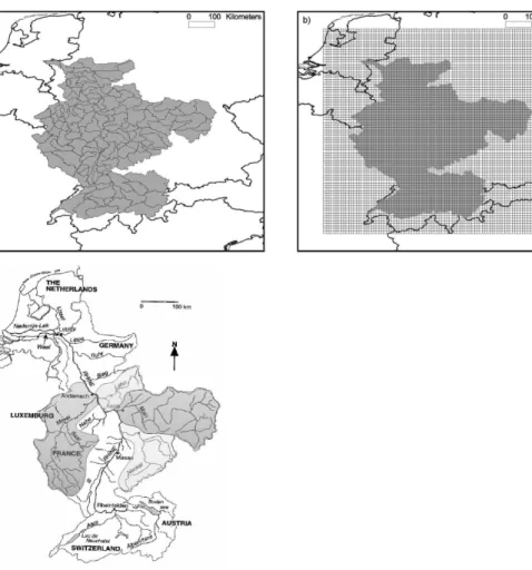
The study area includes the Rhine basin (Fig. 1) upstream of the Dutch-German bor-der and covers an area of 160 800 km2. The Rhine originates in the Alpine mountains that comprise almost 36 000 km2upstream of Basel, with maximum elevations of more than 4000 m a.s.l. Air temperatures are below zero during the winter season due to this height, and a substantial part of the precipitation is stored as snow. Land cover in 10

the Alps is characterized by agricultural land in the lower regions and by forest, shrubs, meadows, unvegetated areas and glaciers on the higher slopes. The area of the Upper Rhine between Basel and Bingen is hilly, with elevations reaching over 1000 m a.s.l., but with flood plains along the main rivers. In the flood plains there is urban develop-ment, while the hills are mainly forested. The main tributaries Neckar, Main, Moselle, 15

Lahn and Sieg have a mixed land use pattern, with agriculture and vineyards on the valley slopes, and forest on the hillslopes and mountains. The Middle Rhine has in-cised in higher grounds, which resulted in a deep narrow valley without floodplains. The relatively flat and low-lying Lower Rhine area downstream of Cologne until the Dutch-German border is an urbanized area with a mixture of agriculture, meadows and 20

some forest. Overall, the Rhine basin is densely settled, with an average population density of 270 persons per km2(Earle, 2001). About 50% of the basin is used for agri-culture, 15–20% is urban or suburban land, and the remainder is forest and otherwise natural lands (Wessel, 1995).

The average discharge of the Rhine at Lobith is 2206 m3/s (1989–1995). The mean 25

(9)

HESSD

4, 4325–4360, 2007

Rhine basin

Title Page

Tables Figures

◭ ◮

Back Close

Full Screen / Esc

EGU

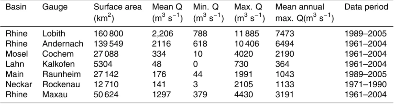
held. Earlier considerable and some catastrophic floods in history are 1421, 1845, 1882 and 1926 (Disse and Engel, 2001). The surface area of the sub-basins under consideration in the present study vary from 5304 km2 to 27 142 km2, as can be seen from Table 1 among other basin characteristics.

4 Methods 5

4.1 Data

Both the HBV and VIC models were forced using downscaled ECMWF ERA15 atmo-spheric re-analysis data, which is provided by the Max Planck Institute for Meteorology (MPI), Hamburg, Germany. The regional climate model REMO (Jacob, 2001) was used for downscaling and this dataset will be further referred to as ERA15. The ERA15 10

data set comprises the years 1993 through 2003, at a 3-hourly time step, with a grid resolution of 0.088 degrees and provides the following forcing data: precipitation, tem-perature, specific humidity, air pressure, downward radiation (shortwave and longwave) and windspeed. These input data are all required to run the VIC model.

To compare this data to observations, two additional meteorological datasets are 15

available. First, a historical data set is available from the International Commission for the Hydrology of the Rhine basin (CHR). This data set is referred to as CHR and contains daily values of precipitation and temperature for the years 1961 through 1995, which are based on 36 measurement stations throughout the basin (Sprokkereef, 2001). Second, a historical dataset using interpolated measured data is available from 20

the Climate Research Unit (CRU) where they develop a number of global datasets widely used in climatic research. This data set is referred to as CRU (Mitchell and Jones, 2005) and contains precipitation and temperature values at a monthly time step and comprises the years 1900 through 1998, with a grid resolution of 0.5 degrees.

Due to the detailed requirements of the VIC model, VIC was only forced by ERA15 25

(10)

HESSD

4, 4325–4360, 2007

Rhine basin

Title Page

Tables Figures

◭ ◮

Back Close

Full Screen / Esc

Interactive Discussion and at least monthly mean values of potential evaporation as input data. Therefore

HBV was forced by both ERA15 and CHR data and precipitation values of the CRU data set were only used for comparison of forcing data.

Additional spatial information on altitude, soil types and land cover is derived from a GIS database available at Federal Institute of Hydrology in Germany (Eberle et al., 5

2005). Historical discharge data was provided by the Dutch governmental Institute for Inland Water Management and Waste Water Treatment (RIZA).

4.2 Forcing data comparison

Rainfall amounts of the three forcing datasets were compared for the period of 1993– 1995; the only three years the three datasets all overlap. A first comparison was made 10

for basin wide mean values at a daily basis between the ERA15 and CHR values. For the second comparison, the ERA15 and CHR data sets were aggregated to weekly and monthly values and then compared to the CRU data.

4.3 Model performance

4.3.1 Calibration at Lobith 15

We forced both models with ERA15 data and calibrated for the discharge gauge at the Dutch-German border at Lobith (see Fig. 1c) using observed discharge at Lobith for the year 1993. Only one year was used in order to limit the amount of calibration time for the VIC model. Because 1993 contains a relatively dry summer, as well as an extreme peak in winter, it was considered representative of the extremes for the total 20

period. The model simulations were initialized using model states of October 1993 and also the first two months of 1993 are considered as a “warm-up” period, hence model results for this period were not used in the calibration process.

(11)

HESSD

4, 4325–4360, 2007

Rhine basin

Title Page

Tables Figures

◭ ◮

Back Close

Full Screen / Esc

EGU

seven parameters describe the layer depths, relations between soil moisture content and baseflow and the infiltration capacity. For a complete description, see Hurkmans (2007).

The original calibration process for the HBV model of the Rhine basin is described by Eberle (2005). HBV was recalibrated in a stepwise approach also using the ERA15 5

dataset for 1993. Based on results of a parameter sensitivity analysis by Passchier and Stone (2003), for HBV, only the parametersfc (field capacity that represents the total water storage capacity of the soil) andkhq (describing the quick runofffunction) were adjusted for recalibration.

4.3.2 Sub-basin scale validation performance 10

The calibrated models are validated using the remaining period of the ERA15 data set, the years 1994 through 2003. There is a large number of efficiency criteria to choose from for model validation, such as those presented by Krause (2005) and each criterion may place different emphasis on different types of simulated and observed behaviours. The objective performance criteria used in the current study to compare the integral 15

time series for the locations, are the coe_fficient of e_fficiency (E) (Nash and Sutcli_ffe, 1970), the coefficient of determination (r2_{) and the volume error (}V_E_).

Model performance differs with the scale on which it is applied. In the present study we are interested in discharges at Lobith (the outlet of the basin), discharges upstream in the main Rhine channel and model performance at the sub-basin scale. The dis-20

charge gauges that were used in the analyses are Lobith, Andernach and Maxau along the Rhine branch, and tributary gauging stations at Cochem (Moselle), Kalkofen (Lahn), Raunheim (Main) and Rockenau (Neckar). These locations are shown in Fig. 1 and characteristics of the sub-basins upstream of those gauges are presented in Ta-ble 1.

(12)

HESSD

4, 4325–4360, 2007

Rhine basin

Title Page

Tables Figures

◭ ◮

Back Close

Full Screen / Esc

Interactive Discussion 4.3.3 Peak flows and low flows

Periods with extreme discharges are often of most interest both in impact studies and real time flow predictions. A good representation by the model of the absolute amount, the timing and duration of the peak and low flows is very relevant. Subsequently, just for the gauge at Lobith, we selected five peak flow and five low flow periods, and 5

chose additional performance indicators that relate to magnitude and timing of peak flows, together with minimum values and duration of low flows. These indicators are observed maximum discharge (max.Q_obs), relative di_fference between observed and simulated maximum discharge (d_max. Q_sim_{), di}_ff_{erence in peak timing (}d T_{), observed}

minimum discharge (min.Q

obs), relative difference between observed and simulated

10

minimum discharge (dmax.Q_sim) and duration of the low flow period under a threshold of 1300 m3/s (DUT). A discharge of 1300 m3/s at Lobith is a critical value in summer periods; lower discharges a_ffect shipping industry, agricultural supply, electricity pro-duction and drinking water supplies.

5 Results 15

5.1 Forcing data comparison

The difference between measured precipitation data (CHR and CRU) and reanalysis data (ERA15) provides an indication for the error or bias in the reanalysis data set. The assumption here is that measured data better represents actual values than reanalysis data and to test this assumption both measured datasets are compared with ERA15 20

(13)

HESSD

4, 4325–4360, 2007

Rhine basin

Title Page

Tables Figures

◭ ◮

Back Close

Full Screen / Esc

EGU

higher than between ERA15 and CRU (r2₌0.65). The correlation between CHR and CRU, however, has anr2 _{value of 0.84, which indicates that these two databases are}

most alike and that ERA15 probably has a larger error than the measured data.

5.2 Model performance

5.2.1 Calibration and validation period at Lobith 5

Daily values of all performance criteria for Lobith are displayed in Table 2, where a distinction is made between the calibration and the validation period. The additional six locations will be discussed in Sect. 5.2.2. At Lobith after calibration, the results of the HBV model forced with ERA15 show a moderate performance (E₌0.49,r2₌0.75), whereas the VIC model fits less well (E₌0.47, r2₌0.64). This is mainly caused by an 10

overestimation of the volume, by 23% (VIC) and 32% (HBV), respectively. However, the HBV model forced with CHR fits well when compared to observed discharges (E₌_0.85, r2₌0.97).

Figure 4 depicts the results of the period 1993–2003 at Lobith, respectively for the VIC and the HBV models both forced with ERA15 data. The HBV model shows a better 15

fit of the simulated discharge to the observed discharge than VIC, which is confirmed by the efficiency coefficients as shown in Table 2. The coefficient of efficiency (E_{) of}

HBV is 0.62, where VIC shows 0.31 and coe_fficient of determination (r2_{) of HBV is 0.65,}

where VIC displays 0.54. The volume error of both models is low (−4% by HBV and 8% by VIC). The VIC model overestimates many peak discharges and underestimates 20

baseflow periods, while the HBV model simulates the baseflow very well and shows a variable performance on flood peaks. The sensitivity of both models to di_fferent meteorological conditions suggests that the storage capacity is underestimated in the upper layers, resulting in too much direct runoffand that the depletion factor controlling drainage from the lower layers is too large.

25

(14)

HESSD

4, 4325–4360, 2007

Rhine basin

Title Page

Tables Figures

◭ ◮

Back Close

Full Screen / Esc

Interactive Discussion considerable negative influence on the performance indicators. Nonetheless, when

monthly values of simulated discharge are evaluated they display similar or slightly worse results, as can be seen from Table 2; VIC and HBV forced with ERA15 perform moderate and HBV forced with CHR fits well, which is about equal to the HBV simula-tions at a daily basis. The di_fference in coe_fficient of e_fficiency (E_{) between daily and}

5

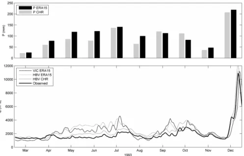
monthly values of the HBV model forced with ERA15 in the calibration period stands out though, a moderate 0.49 for daily values and a dramatic−0.08 for monthly values. Instead of the expected damping e_ffect on performance, aggregating to a bigger time step indeed causes the observed and modelled peak value of several days in Decem-ber 1993 (shown in Fig. 3) to damp, but does not effect the more or less consistent 10

over estimation during the months May until July. Since the coe_fficient of e_fficiency (E₎

is sensitive to peak values, in this case the absolute observed and modelled discharge values are damped, but the relative error by time step increases which causes the coe_fficient to drop.

These results indicate that forcing data largely influence the performance values of 15

both models. A closer examination of the precipitation values in both forcing data sets during the calibration period is depicted in Fig. 3, together with observed and simulated discharge values. The figure shows that during the months May, June and July, both HBV and VIC forced with ERA 15 consistently overestimate discharge by 25–100%, whereas HBV forced with CHR also overestimates discharge, but to a lesser degree. 20

This can be explained by the equally consistent higher ERA15 precipitation values when compared to the CHR data. In August, ERA15 again displays higher values than the CHR data, while observed and simulated discharge agree quite well. This lack of reaction in modelled discharge in August can be explained by higher evaporation values during summer than spring, which neutralize the precipitation surplus, next to 25

(15)

HESSD

4, 4325–4360, 2007

Rhine basin

Title Page

Tables Figures

◭ ◮

Back Close

Full Screen / Esc

EGU

5.2.2 Sub-basin scale performance

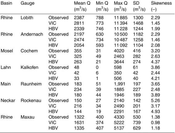
Several statistical parameters for the complete simulation period are presented in Ta-ble 3. The mean and minimum simulated discharges agree reasonaTa-ble well for the HBV model, whereas VIC overestimates those values, except for the gauges at Cochem and Kalkofen. The maximum discharges, though, are underestimated for most locations, 5

except for the most upstream gauges Rockenau and Maxau. The values for the stan-dard deviation (SD) based on daily values are high for both simulated and observed values. This can be explained by the skewed distribution of the discharge values. Based on this information it can be concluded that the probability density function of the observed values at Lobith is best represented by the simulated discharges by HBV. 10

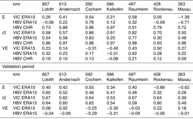
For the remaining six gauges upstream of Lobith, scatter plots of the daily observed and simulated discharges are displayed (Fig. 5) for the validation period. The acces-soryr2 values are presented in Table 4. Table 4 and 5 show the results of all perfor-mance criteria for daily and monthly values respectively, for all locations. Above the location name, thekmr number is displayed. This number represents the length of the 15

Rhine from the Bodensee in Switzerland and Germany. For example, the gauging sta-tion at Lobith is located 857 km downstream form the Bodensee. In the current study, the gauges that are not located exactly along the Rhine, but along tributaries draining the sub-basins, havekmr numbers that represent locations where the side rivers enter the Rhine. Thekmr number is used to illustrate all performance criteria as presented 20

in Table 4 and 5, in a graphical way in Fig. 6 and Fig. 7. In Fig. 7, the volume error is not displayed, since the volume error does not change when the time step is adjusted (see Tables 4 and 5).

The Nash & Sutcliffe efficiency coefficient (E_{) decreases in the upstream direction,}

sometimes even below zero at Rockenau and Maxau for VIC results. An e_fficiency 25

(16)

HESSD

4, 4325–4360, 2007

Rhine basin

Title Page

Tables Figures

◭ ◮

Back Close

Full Screen / Esc

Interactive Discussion better than both models forced with ERA15. Moreover, for the ERA15 forcing, HBV

performs marginally better than VIC at a daily basis, whereas VIC performs marginally better than HBV at a monthly basis. When studying the validation period on the right side, however, HBV performs substantially better than VIC, which indicates that HBV is more robust in its performance.

5

5.2.3 Peak flows and low flows

Table 6 shows the five highest daily discharges and the five lowest monthly discharges, as observed and simulated at Lobith. Observed volumes over threshold and maximum peak discharges reveal that both models overestimate and underestimate the same peaks. Furthermore, it shows that VIC tends to delay flood peaks, for some peaks 10

even up to 6 days, while HBV simulates the timing of the peaks very well. Two factors in VIC explain this delaying of peak flows: first, the routing algorithm that is used in VIC might delay arrival at Lobith slightly compared to the internal routing algorithm in HBV. This was also noted in Hurkmans et al. (2007) where runofffrom another conceptual water balance model (STREAM) was routed with di_fferent algorithms. Second, the de-15

gree to which peaks are delayed also depends on calibration parameters, particularly depths of the upper layers and the infiltration capacity factor (see for details on VIC calibration Hurkmans et al., 2007). When the resulting infiltration capacity is higher, there is less direct runo_ffand, in case of near-saturation, excess water is, with a small delay, transported as baseflow. For the peak of 1993, which is included in the calibra-20

tion period, the simulated timing by VIC was rather accurate, however, for other peaks in the validation period these parameter settings were apparently less applicable.

Concerning the low flows, VIC tends to underestimate the minimum values and HBV tends to overestimate the low flows under consideration. For the duration of the most extreme low flows below a threshold of 1300 m3/s, both models underestimated the 25

(17)

HESSD

4, 4325–4360, 2007

Rhine basin

Title Page

Tables Figures

◭ ◮

Back Close

Full Screen / Esc

EGU 6 Discussion and conclusions

In the view of the utility of hydrological models in climate scenario studies, the goal of this paper was to compare the hydrological models HBV and VIC by testing their performance for simulating historical discharge in the Rhine basin. These models have di_fferent model structures and there is no consensus in research on rainfall-runo_ff mod-5

elling on what model structure is to be preferred. Some research suggest, however, that the VIC approach more accurately simulates the timing of peak discharges (Troy et al., 2007). Di_fferent meteorological data sets were used as model input and HBV and VIC were compared at both basin and sub-basin scale using various performance criteria. Furthermore, simulated peak flows and low flows were compared.

10

We have seen that the performance of both models was less in upstream basins than at the basin outlet (gauging station Lobith), but that for all upstream basins HBV still performed better than VIC at a daily basis. We have seen that HBV was more robust when the performance of the calibration period (E₌0.49,r2₌0.75 vs.E₌0.47,r2₌0.64 at Lobith) and the validation period (E₌_0.62, r2₌_{0.65 vs.}E₌_0.31, r2₌_{0.54 at Lobith)}

15

were compared. In addition, HBV forced with CHR data performed much better than both VIC and HBV forced with ERA15 (E₌0.85, r2₌0.97 for the calibration period at Lobith).

For the most extreme peak flows, HBV simulated maximum discharges best (dmax. Q_simHBV 1–17%,dmax.Q_simVIC 2–27%), while VIC performed better at the 20

moderate peak flows (d_max. Q_sim _{HBV 21–35%,} d_max. Q_sim _{VIC 13–35%). Besides}

simulating measured values of discharges, timing of peak flows was investigated. It appeared that VIC displayed several days delay in estimating timing of the peak dis-charge. Most low flows were underestimated by VIC, where HBV showed overestima-tion of the low flows. Also the performance of both models in reproducing duraoverestima-tion of 25

low flows was poor.

(18)

HESSD

4, 4325–4360, 2007

Rhine basin

Title Page

Tables Figures

◭ ◮

Back Close

Full Screen / Esc

Interactive Discussion idea that more complex physically-based distributed modelling better represents

ob-served discharges as compared to simple conceptual model approaches (Reggiani and Schellekens, 2003; Refsgaard, 1996). These results support the notion that even for a well documented river basin such as the Rhine, more complex modelling does not automatically lead to better results (Booij, 2003; Uhlenbrook, 2003).

5

We are convinced, though, that VIC should be able to perform better than it has done so far in the Rhine basin, and thus model performance might be improved (Hurkmans et al., 2007). The performance of VIC might increase using a longer calibration period and further refining the spatial distribution of adjusted parameters. Furthermore, by solving both the water and the energy balance VIC holds the potential to better de-10

scribe soil-atmosphere feedback processes, if the model scheme were to be combined with an atmospheric model. In the line of small-scale hydrometeorology and modelling the effects of land use change, this is a conclusive reason for further development (Hurkmans et al., 2007). Moreover, VIC has performed well in the past, for example in studies by Liang et al. (1994) and Troy et al. (2007). But also the HBV model for the 15

Rhine basin can be improved. Lake retention for example, is not implemented yet in both models. Especially concerning the Bodensee, a large upstream lake in the Rhine basin, this is a quite drastic simplification and an obvious potential for further improve-ment. We subscribe the recommendation of (Seibert, 1999), that model development and calibration is an undertaking that should not be carried out by a single researcher, 20

but requires scientific dialogue.

The results also lead us to the conclusion that forcing data has a considerable influ-ence on model performance, irrespectively to the type of model structure. It empha-sizes the need for ground-based meteorological measurements and a suggestion might be to correct downscaled climate model re-analyses data such as ERA15, whenever 25

(19)

HESSD

4, 4325–4360, 2007

Rhine basin

Title Page

Tables Figures

◭ ◮

Back Close

Full Screen / Esc

EGU

shows a climate model’s ability to simulate the 95th rainfall percentile. Comprehensive comparison and correction of downscaled climate model output is a challenging task for further research.

The conclusion as to the application of hydrological models in climate scenario stud-ies, then, is that for the Rhine basin HBV is preferred, since it has shown better overall 5

performance and seems to be more robust than VIC. The extreme events were sim-ulated best by HBV, which implies that HBV can provide the most reliable indication of possible future shifts in extreme events due to climate change. The more realistic representation of evaporation processes by VIC than HBV did not result in better per-formance even in the dry periods, when the evaporation volume is substantial in the 10

water balance. The final advantage of HBV over VIC is that HBV has short computa-tion times, which makes it suitable for simulating long time series of the many available different climate scenarios.

Acknowledgements. This research was supported by the project ACER (A7) under the Dutch

BSIK Climate Changes Spatial Planning program. We wish to thank H. Buiteveld from the Dutch 15

Institute for Inland Water Management and Waste Water Treatment (RIZA) and the German Federal Institute of Hydrology (BfG) for both allowing the use of the HBV model, and providing meteorological and discharge measurement data. D. Jacob and E. Mazurkewitz from the Max Planck Institute for Meteorology are kindly acknowledged for providing meteorological data. Finally we thank two anonymous colleagues for occasional data editing and their constructive 20

comments that helped to improve this paper.

References

Abbott, M. B., Bathurs, J. C., Cunge, J. A., O’Connel, P. E., and Rasmussen, J.: An intro-duction to the european hydrological system – systeme hydrologique “She”, 1: History and philosophy of a physically based distributed modelling system, J. Hydrol., 87, 45–59, 1986. 25

(20)

HESSD

4, 4325–4360, 2007

Rhine basin

Title Page

Tables Figures

◭ ◮

Back Close

Full Screen / Esc

Interactive Discussion Bergstr ¨om, S., Lindstr ¨om, G., and Pettersson, A.: Multi-variable parameter estimation to

in-crease confidence in hydrological modelling, Hydrol. Process., 16, 413–421, 2002.

Beven, K.: How far can we go in distributed hydrological modelling?, Hydrol. Earth Syst. Sci., 5, 1–12, 2001,

http://www.hydrol-earth-syst-sci.net/5/1/2001/. 5

Beven, K.: Towards an alternative blueprint for a physically based digitally simulated hydrologic response modelling system, Hydrol. Process., 16, 189–206, 2002a.

Beven, K.: Towards a coherent philosophy for modelling the environment, Proc. R. Soc. Lond. A, 458, 1–20, 2002b.

Bogaard, T. A., Luxemburg, W. M. J., De Wit, M., Douben, N., and Savenije, H. H. G.: Some 10

hydrological challenges in understanding discharge generation processes in the Rhine and Meuse basins, Phys. Chem. Earth, 30, 262–266, 2005.

Booij, M. J.: Determination and integration of appropriate spatial scales for river basin mod-elling, Hydrol. Process., 17, 2581–2598, 2003.

Buishand, T. A. and Lenderink, G.: Estimation of future discharges of the river Rhine in the 15

SWURVE project, KNMI, De Bilt, The Netherlands TR-273, 1–36, 2004.

Disse, M. and Engel, H.: Flood events in the Rhine basin: Genesis, influendes and mitigation, Nat. Hazards, 23, 271–290, 2001.

The water page – the Rhine river: http://www.thewaterpage.com/rhine main.htm, access: 2 April 2007, 2001.

20

Eberle, M., Buiteveld, H., Wilke, K., and Krahe, P.: Hydrological modelling in the river Rhine basin part iii - daily HBV model for the Rhine basin, Institute for Inland Water Management and Wase Water Treatment (RIZA) and Bundesanstalt f ¨ur Gew ¨asserkunde (BfG), Koblenz, Germany BfG-1451, 2005.

Hurkmans, R. T. W., De Moel, H., Aerts, J. C. J. H., and Troch, P. A.: Water balance model 25

versus land surface scheme to model river Rhine discharges, Water Resour. Res., accepted, 2007.

Jacob, D.: A note to the simulation of the annual and inter-annual variability of the water budget over the baltic sea drainage basin, Meteorol. Athos. Phys., 77, 61–73, 2001.

Jothityangkoon, M., Sivalapan, M., and Farmer, D. L.: Process controls of water balance vari-30

ability in a large semi-arid catchment: Downward approach to hydrological model develop-ment, J. Hydrol., 254, 174–198, 2001.

(21)

HESSD

4, 4325–4360, 2007

Rhine basin

Title Page

Tables Figures

◭ ◮

Back Close

Full Screen / Esc

EGU

model assessment, Adv. Geosci., 5, 89–97, 2005, http://www.adv-geosci.net/5/89/2005/.

Kundzewicz, Z. W., Mata, L. J., Arnell, N. W., D ¨oll, P., Kabat, P., Jim ´enez, B., Miller, K. A., Oke, T., Sen, Z., and Shiklomanov, I. A.: Freshwater resources and their management, in: Climate change 2007: Impacts, adaptation and vulnerability, Contribution of working group 5

ii tot the fourth assessment report of the intergovernmental panel on climate change, edited by: Parry, M. L., Conziani, O. F., Palutikof, J. P., Van der Linden, P. J., and Hanson, C. E., Cambridge University Press, Cambridge, UK, 173–210, 2007.

Kwadijk, J. C. J.: The impact of climate change on the discharge of the river Rhine, PhD Thesis, University of Utrecht, Utrecht, The Netherlands, 1993.

10

Liang, X., Lettenmaier, D. P., Wood, E. F., and Burges, S. J.: A simple hydrologically based model of land surface water and energy fluxes for general circulation models, J. Geophys. Res., 99, 415–428, 1994.

Liang, X., and Zhenghui, X.: A new surface runoff parameterization with subgrid-scale soil heterogeneity for land surface models, Adv Water Resour, 24, 1173-1193, 2001.

15

Lindstr ¨om, G., Johansson, B., Persson, M., Gardelin, M., and Bergstr ¨om, S.: Development and test of the distributed HBV-96 hydrological model, J. Hydrol., 201, 272–288, 1997.

Lohmann, D., Nolte-Holube, R., and Raschke, E.: A large-scale horizontal routing model to be coupled to land surface parametrization schemes, Tellus, 48A, 708–721, 1996.

Middelkoop, H., Daamen, K., Gellens, D., Grabs, W., Kwadijk, J. C. J., Lang, H., Parmet, B. 20

W. A. H., Sch ¨adler, B., Schulla, J., and Wilke, K.: Impact of climate change on hydrological regimes and water resources management in the Rhine basin., Climatic Change, 49, 105– 128, 2001.

Mitchell, T. D. and Jones, P. D.: An improved method of constructing a database of monthly climate observations and associated high-resolution grids, Int. J. Climatol., 25, 693–712, 25

2005.

M ¨ulders, R., Parmet, B., and Wilke, K.: Hydrological modelling in the river Rhine basin. Final report, Federal Institute of Hydrology (BfG), KoblenzBfG – 125, 1999.

Nash, J. E. and Sutcliffe, J. V.: River flow forecasting through conceptual models. Part i – a discussion of principles, J. Hydrol., 10, 282–290, 1970.

30

Passchier, R. and Stone, K.: Analysis of the instrumentation for computing design discharges, WL|Delft Hydraulics, Delft, The Netherlands, Q2705, 1–78, 2003.

(22)

HESSD

4, 4325–4360, 2007

Rhine basin

Title Page

Tables Figures

◭ ◮

Back Close

Full Screen / Esc

Interactive Discussion model performance? Comparative assessments of common catchment model structures on

429 catchments, J. Hydrol., 242, 275–301, 2000.

Pitman, A. J. and Perkins, S. E.: Reducing uncertainty in selecting climate models for hy-drological impact assessments, in: Quantification and Reduction of Predictive Uncertainty for Sustainable Water Resource Management, Symposium HS2004 at IUGG2007, Perugia, 5

3–15, 2007.

Refsgaard, J. C.: Terminology, modelling protocol and classification of hydrological model codes, in: Distributed hydrological modelling, edited by: Abbott, M. B. and Refsgaard, J. C., Kluwer Academic Publishers, 17–39, 1996.

Reggiani, P., Hassanizadeh, S. M., Sivapalan, M., and Gray, W. G.: A unifying framework for 10

watershed thermodynamics: Balance equations for mass, momentum, energy and entropy, and the second law of thermodynamics, Adv. Water Resour., 22, 367–398, 1998.

Reggiani, P., Hassanizadeh, S. M., Sivapalan, M., and Gray, W. G.: A unifying framework for watershed thermodynamics: Constitutive relationships, Adv. Water Resour., 23, 15–39, 1999.

15

Reggiani, P. and Schellekens, J.: Modelling of hydrological responses: The respresentative elementary watershed approach as an alternative blueprint for watershed modelling, Hydrol. Process., 17, 3785–3789, 2003.

Rientjes, T. and Zaadnoordijk, W. J.: Hoogwatervoorspelling: Fysisch gebaseerde regen-afvoermodellering. Dilemma of d ´ej `a vu?, Stromingen, 6, 33–44, 2000 (in Dutch).

20

Savenije, H. G.: Equifinality, a blessing in disguise?, Hydrol. Process., 15, 2835–2838, 2001. Sch ¨ar, C., L ¨uthi, D., Beyerly, U., and Heise, E.: The soil-precipitation feedback: A process study

with a regional climate model, J. Climate, 12, 722–741, 1998.

Schulla, J. and Kaspar, K.: Model description wasim-eth, Internal report, IAC, ETH, Z ¨urich, 1–174, 2006.

25

Seibert, J.: Conceptual runoff models - fiction or representation of reality, MSc Thesis, Acta University, Uppsala, Sweden, 52 pp., 1999.

Shaw, E. M.: Hydrology in practice, Nelson Thornes Ltd, Cheltenham, England, 1–569, 2002. Sprokkereef, E.: Eine hydrologische datenbank f ¨ur das Rheingebiet, International Commission

for the Hydrology of the Rhine Basin (CHR), 2001. 30

(23)

HESSD

4, 4325–4360, 2007

Rhine basin

Title Page

Tables Figures

◭ ◮

Back Close

Full Screen / Esc

EGU

Troy, T., Sheffield, J., and Wood, E.: Temporal and spatial scales in hydrological model calibra-tion, in: Geophysical Research Abstracts, European Geosciences Union General Assembly 2007, Vienna, Austria, 2007,

Uhlenbrook, S., Seibert, J., Leibundgut, C., and Rodhe, A.: Prediction uncertainty of concep-tual rainfall-runoffmodels caused by problems to identify model parameters and structure, 5

Hydrol. Sci., 44, 779–798, 1999.

Uhlenbrook, S.: An emperical approach for delineating spatial units with the same dominating runoffgeneration processes, Phys. Chem. Earth, 28, 297–303, 2003.

Van Deursen, W. P. A. and Kwadijk, J. C. J.: Rhineflow: An integrated GIS water balance model for the river Rhine, HydroGIS 93: Application of Geographic Information Systems in 10

Hydrology and Water Resources, 507–518, 1993.

Van Deursen, W. P. A.: Rapportage Rhineflow/Meuseflow. Nieuwe KNMI scenario’s mei 2006,, Carthago Consultancy, Rotterdam, the Netherlands, 2006 (in Dutch).

Wagener, T., McIntyre, N., Lees, M. J., Wheater, H. S., and Gupta, H. V.: Towards reduced uncertainty in conceptual rainfall-runoffmodelling: Dynamic identifiability analysis, Hydrol. 15

Process., 17, 455–476, 2003.

Ward, R. C. and Robinson, M.: Principles of hydrology, 4 ed., McGraw-Hill Publishing Company, London, 2000.

Weerts, A. H.: Assessing and quantifying the combined effect of model parameter and bound-ary uncertainties in model based flood forecasting., Geophys. Res. Abstr., 5, 14564, 2003. 20

Weerts, A. H. and Van der Klis, H.: FEWS-Rhine version 1.02. Improvements and adjustments., WL|Delft Hydraulics, DelftQ3618, 2004.

(24)

HESSD

4, 4325–4360, 2007

Rhine basin

Title Page

Tables Figures

◭ ◮

Back Close

Full Screen / Esc

Table 1.Basin and sub-basin characteristics. Surface area (km2) is defined by the basin area upstream of the gauging station.

Basin Gauge Surface area Mean Q Min. Q Max. Q Mean annual Data period (km2) (m3s−1) (m3s−1) (m3s−1) max. Q(m3s−1)

(25)

HESSD

4, 4325–4360, 2007

Rhine basin

Title Page

Tables Figures

◭ ◮

Back Close

Full Screen / Esc

EGU

Table 2. Performance criteria daily and monthly values at Lobith for the calibration period (March 1993–December 1993) and te validation period (1994–2003).

Calibration period Validation period daily monthly daily monthly

E VIC ERA15 0.47 0.26 0.31 0.40 HBV ERA15 0.49 −0.08 0.62 0.60 HBV CHR 0.85 0.73 – – r2 VIC ERA15 0.64 0.58 0.54 0.67

HBV ERA15 0.75 0.54 0.65 0.64 HBV CHR 0.97 0.96 – – VE VIC ERA15 0.23 0.23 0.08 0.08

(26)

HESSD

4, 4325–4360, 2007

Rhine basin

Title Page

Tables Figures

◭ ◮

Back Close

Full Screen / Esc

Table 3. Observed and simulated mean, minimum and maximum discharge (in m3/s), their standard deviation (SD) and skewness for the period March 1993 through December 2003.

Basin Gauge Mean Q Min Q Max Q SD Skewness (m3/s) (m3/s) (m3/s) (m3/s) (–)

(27)

HESSD

4, 4325–4360, 2007

Rhine basin

Title Page

Tables Figures

◭ ◮

Back Close

Full Screen / Esc

EGU

Table 4.Performance criteria daily values.

Calibration period

kmr 857 613 592 586 497 428 363 Lobith Andernach Cochem Kalkofen Raunheim Rockenau Maxau

E VIC ERA15 0.47 0.52 0.45 0.24 0.64 −0.16 −1.20 HBV ERA15 0.49 0.59 0.81 0.30 0.60 0.31 −0.40 HBV CHR 0.85 0.91 0.92 0.86 0.89 0.77 0.78 r2 VIC ERA15 0.64 0.61 0.57 0.50 0.76 0.40 0.47 HBV ERA15 0.75 0.75 0.82 0.37 0.83 0.48 0.54 HBV CHR 0.97 0.97 0.95 0.86 0.96 0.88 0.95 VE VIC ERA15 0.23 0.14 -0.31 -0.49 0.43 0.50 0.27 HBV ERA15 0.32 0.23 0.17 −0.31 0.62 0.28 0.22 HBV CHR 0.19 0.10 0.13 −0.08 0.21 0.12 0.09

Validation period

(28)

HESSD

4, 4325–4360, 2007

Rhine basin

Title Page

Tables Figures

◭ ◮

Back Close

Full Screen / Esc

Table 5.Performance criteria monthly values.

Calibration period

E VIC ERA15 0.26 0.41 0.54 0.21 0.58 0.05 −1.39 HBV ERA15 −0.08 0.22 0.78 0.13 0.32 −0.09 −0.71 HBV CHR 0.73 0.88 0.96 0.97 0.91 0.79 0.72 r2 VIC ERA15 0.58 0.57 0.86 0.61 0.82 0.70 0.50 HBV ERA15 0.54 0.58 0.83 0.20 0.77 0.30 0.48 HBV CHR 0.96 0.97 0.98 0.97 0.98 0.93 0.96 VE VIC ERA15 0.23 0.14 −0.31 −0.49 0.43 0.50 0.27 HBV ERA15 0.32 0.23 0.17 −0.31 0.62 0.28 0.22 HBV CHR 0.19 0.10 0.13 −0.08 0.21 0.12 0.09

Validation period

(29)

HESSD

4, 4325–4360, 2007

Rhine basin

Title Page

Tables Figures

◭ ◮

Back Close

Full Screen / Esc

EGU

Table 6. Analysis of peak flows and low flows at the outlet of the basin (Lobith), showing observed maximum discharge (max. Q_obs), relative difference between observed and simu-lated maximum discharge (dmax. Q_sim), difference in peak timing (d T), observed minimum discharge (min.Q_obs), relative difference between observed and simulated minimum discharge (d_max.Q_sim_{) and duration of the low flow period under a threshold of 1300 m}3_{/s (DUT).}

Peak flows 31/01/1995 25/12/1993 04/11/1998 07/01/2003 28/03/2001

Max.Q_obs_(m3_/s) _{11 775} _{11 034} ₈₄₁₀ ₉₃₆₆ ₈₆₆₆ d_max.Q_sim_{VIC (%)} ₋_26.7 _1.5 ₋_35.1 ₋_15.5 ₋_12.5 d_max.Q_sim_{HBV (%)} ₋_16.3 _0.9 ₋_34.9 ₋_32.1 ₋_20.6

d T VIC (days) 2 2 6 5 4

d T HBV (days) 0 0 0 −1 −1

Low flows 09/2003 11/1997 08/1998 09/1996 03/1993 Min.Q_obs_(m3_/s) ₇₈₈ ₉₃₁ ₉₈₃ ₁₀₇₇ ₁₂₂₈ d_min.Q_sim _{VIC (%)} ₋_20.3 ₋_10.7 _4.5 ₋_-26.0 ₋_38.5 d_min.Q_sim _{HBV (%)} _18.7 _6.5 _44.4 ₋_15.8 _0.5

DUTQ_obs(days) 141 68 39 37 13 DUT VIC (days) 104 22 15 60 68

(30)

HESSD

4, 4325–4360, 2007

Rhine basin

Title Page

Tables Figures

◭ ◮

Back Close

Full Screen / Esc

(31)

HESSD

4, 4325–4360, 2007

Rhine basin

Title Page

Tables Figures

◭ ◮

Back Close

Full Screen / Esc

EGU

(32)

HESSD

4, 4325–4360, 2007

Rhine basin

Title Page

Tables Figures

◭ ◮

Back Close

Full Screen / Esc

(33)

HESSD

4, 4325–4360, 2007

Rhine basin

Title Page

Tables Figures

◭ ◮

Back Close

Full Screen / Esc

EGU

(34)

HESSD

4, 4325–4360, 2007

Rhine basin

Title Page

Tables Figures

◭ ◮

Back Close

Full Screen / Esc

(35)

HESSD

4, 4325–4360, 2007

Rhine basin

Title Page

Tables Figures

◭ ◮

Back Close

Full Screen / Esc

EGU

(36)

HESSD

4, 4325–4360, 2007

Rhine basin

Title Page

Tables Figures

◭ ◮

Back Close

Full Screen / Esc