I
MPUTATION METHODS FOR FILLING MISSING DATA IN
URBAN AIR POLLUTION DATA FOR
M
ALAYSIA
Nur Afiqah ZAKARIA
School of Environmental Engineering, University Malaysia Perlis (UniMAP), Kompleks Pusat Pengajian Jejawi 3, 02600 Arau, Perlis, e-mail: [email protected]
Norazian Mohamed NOOR
Senior Lecturer (PhD), School of Environmental Engineering,University Malaysia Perlis (UniMAP), Kompleks Pusat Pengajian Jejawi 3,02600 Arau, e-mail: [email protected]
Abstract. The air quality measurement data obtained from the continuous ambient air quality monitoring (CAAQM) station usually contained missing data. The missing observations of the data usually occurred due to machine failure, routine maintenance and human error. In this study, the hourly monitoring data of CO, O3, PM10, SO2, NOx, NO2, ambient temperature and humidity were used to evaluate four imputation methods (Mean Top Bottom, Linear Regression, Multiple Imputation and Nearest Neighbour). The air pollutants observations were simulated into four percentages of simulated missing data i.e. 5%, 10%, 15% and 20%. Performance measures namely the Mean Absolute Error, Root Mean Squared Error, Coefficient of Determination and Index of Agreement were used to describe the goodness of fit of the imputation methods. From the results of the performance measures, Mean Top Bottom method was selected as the most appropriate imputation method for filling in the missing values in air pollutants data.
Key words: air pollution, missing data, imputation methods, multiple imputation.
1. Introduction
Air pollution is the condition where the air is contaminated with foreign substances or the substances themselves. According to Md Razak et al. (2013) air pollution could be aerosols or gases with particles or liquid droplets suspended in the air that might change the natural composition of the atmosphere, would be dangerous to human, animals and plants and also caused destruction to land and water bodies.
2006), industrial and power plants and open burning (Azmi et al., 2010), but the most important drivers are demography (Cole and Neumayer, 2004 and urbanization (Dominick et al., 2012). The effects are aggravated by the tropical environment (Azizi et al., 1995). Nevertheless, legislative measures were able to improve the situation (Awang et al., 2000).
Particulate matter (PM10) was recorded as
the most prevailing pollutant in Southeast Asia Region. The particulate matter have an important role both in atmosphere transparency and air purity; they reduce the quality of the environmental factors (Tudose et al.,
2015). There are three main contributors of PM10 in Malaysia i.e. vehicular
emissions, power stations and industrial sectors. Seventy six percent (4585 tonnes) of PM10 emission in Malaysia is from
motor vehicles whereas power plant emission impacted fifteen percent (15 tonnes) and only four percent (4 tonnes) caused by industrial sector. Hence, urban areas with higher amount of vehicles contribute more air pollution compared to rural areas. Furthermore, high PM10
concentrations were detected during dry season or also known as summer monsoon (June to September) due to the vast quantities of smoke releases by biomass burning from regional sources (Nooret al., 2015).
Air quality monitoring of air pollution is very important. This is because, the data from the air quality monitoring will show or detect any significant pollutant concentration. In Malaysia, the Department of Environmental (DOE) is responsible for monitoring the status of air quality, however, this operation is privatized to Alam Sekitar Malaysia Sdn. Bhd. (ASMA).
The data of air quality obtained from the CAAQM stations usually contained missing data that caused bias due to systematic error between observed and unobserved (Noor et al., 2008). Missing data was a very frequent problem happened in many scientific fields above all in environmental researches (Xia et al., 1999).
The missing data would give impact to the result of statistical analysis depending on the mechanism that made the data to be missed and or the way the data analyst deal with them (Devore, 2006; Plaia and Bondì, 2006). Furthermore, missing observations hindered the ability to make exact conclusion or interpretations about the observation (Noor et al., 2015).
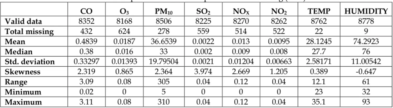
Table 1.Descriptive statistics for all parameters of Bachang (2008).
CO O3 PM10 SO2 NOX NO2 TEMP HUMIDITY
Valid data 8352 8168 8506 8225 8270 8262 8762 8778
Total missing 432 624 278 559 514 522 22 9
Mean 0.4839 0.0187 36.6539 0.0022 0.013 0.0095 28.1245 74.2923
Median 0.38 0.016 33 0.002 0.009 0.008 27.7 76
Std. deviation 0.33297 0.01393 19.79504 0.0021 0.01204 0.00663 2.58171 11.00542
Skewness 2.319 0.865 2.364 3.974 2.669 1.205 0.389 -0.647
Range 3.09 0.08 305 0.04 0.12 0.04 12.1 61
Minimum 0.02 0 5 0 0 0 23 32
Maximum 3.11 0.08 310 0.04 0.12 0.04 35.1 93
The main objective of this research was to find the most appropriate method in filling the missing observations in air pollutant data. A few single imputation methods and multiple imputation method were adopted and the performances of all methods were compared using performance measures.
2. Methodology
2.1. Data In this study, hourly averaged of 5 air pollutants data and 3 meteorological data in Malacca, Malaysia for 2008 were selected. The total observation of these 8 data was 70272 and the total missing data was 2960 (4.212 %). The highest missing observation was found out to be O3
concentration with 624 missing observations. Overall, for the ambient air quality, the daily mean concentration of CO, O3, SO2, NO2 and PM10 were not
exceeding the limit stated in the Malaysia Air Quality Guideline (MAAQG).
Table 1 shows the descriptive statistics for all air pollutants in Malacca (2008). All air pollutants concentration except for humidity, the mean was higher than the median. It indicated that the pollutant distributions were skewed to the right and the extreme events occurred. The mean value for humidity parameter was lower than the median value which meant that the pollutant distributions was skewed to
the left and the skewness value would be negative.
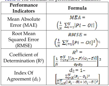
Table 2 shows the mean percentages of the length of gap (in hour) for all air pollutants data. 1-hour gap of missing observation was recorded highest with the value of 92% whereas for missing gap between 1h and 3h, the value reduced drastically to only 4.7%. The higher percentage of missing data in the length of gap more than 15h was due to the missing observations of three parameters in the gaps of between 51h to 54h.
Table 2.Percentage of the length of gap (hour). Length of gap (hour) Percent (%)
l =1 91.642
1 <l < 3 4.717 3 <l < 6 0.953
6<l < 9 0.260
9 <l < 12 0.236 12 > l > 15 1.805
l >15 0.387
2.3. Imputation methods Four imputation methods were used to fill in the simulated missing data. The methods used were Mean Top Bottom, Nearest Neighbour, Linear Regression and Multiple Imputation Method. Multiple Imputation method was carried out to compare the performances of single imputation methods with Multiple Imputation methods.
2.3.1. Mean Top Bottom Mean Top Bottom or also known as Mean Before After method was the average of one existing observation on the top and the bottom of the missing values (Noor et al., 2015). The equation was written as (Nooret al., 2015):
(1)
2.3.2. Nearest Neighbour Nearest Neighbour was the method to replace the missing data with the nearest value to the missing datum (Noor et al., 2015). Nearest Neighbour imputation was the simplest method available, in that the end points of the gaps were used as estimates for all the missing values. The equation is (Junninenet al., 2004);
if / 2
if / 2 (2)
2.3.3. Linear Regression Linear Regression is a model that has relationship between the two variables by fitting a linear equation to the observed data. The missing value of the data will be replaced by regression of the unobserved variables against observed one for that dataset (Noor et al., 2015). The equation is represented as (Noor et al., 2015):
(3)
2.3.4. Multiple Imputation Multiple Imputation methods is the method that generate multiple simulated values for each of the missing data. Multiple imputation by Markov chain Monter Carlo (MCMC) was used in this study and it was conducted by using SPSS. MCMC is used to generate pseodorandom draws from multidimensional dataset and then, complicated probability distributions were generated via Markov chains (Schafer, 1997).
Table 3.The formulas for performance indicators Performance
Indicators Formula
Mean Absolute Error (MAE)
=
Root Mean Squared Error
(RMSE)
=
½
Coefficient of Determination (R²)
=
Index Of Agreement (d2)
d2= –
agreement (d2). Table 3 shows the
formula for performance indicators.
Where is the number of imputation, is the observed data points, the imputated data point, is the average of imputed data, is the average of observed data, is the standard deviation of the imputed data and is the standard deviation of the observed data.
4. Results and discussion
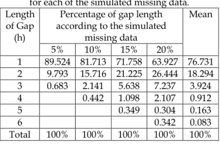
4.1. Characteristics of the simulated data Table 4 shows the percentages of the gap length (in hour) for different percentages of simulated missing observations. The simulated missing data were constructed according to the real missing data trend as shown in Table 2. The maximum number of gaps were limited to 5 hour due to the signifant percentages of the missing gap were between 1 h to 5h (Table 2). Hence, the increment of the gap length percentages are gradually increased as the percentages of simulated missing data increases.
Table 4. The percentage of the gap length (hour) for each of the simulated missing data.
Percentage of gap length according to the simulated
missing data Length
of Gap (h)
5% 10% 15% 20%
Mean
1 89.524 81.713 71.758 63.927 76.731 2 9.793 15.716 21.225 26.444 18.294 3 0.683 2.141 5.638 7.237 3.924
4 0.442 1.098 2.107 0.912
5 0.349 0.304 0.163
6 0.342 0.083
Total 100% 100% 100% 100% 100%
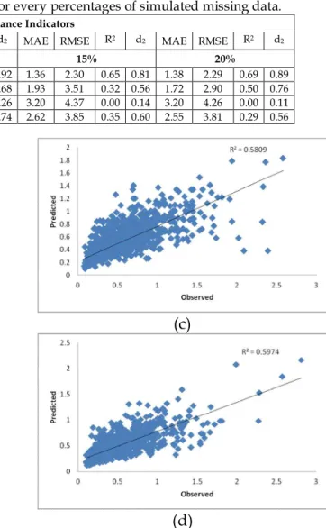
4.2. The best imputation method Overall, based on the results in Table 5, it shows that the error (MAE and RMSE) would be increased and the measure of performances (R2 andd2) decreased as the
percentages of simulated missing data increases. This was consistence with the statement reported by Junger and de
Leon (2015) that the validity of the estimates would be decreased when the missing values increased.
The best imputation method for estimating the simulated missing data was Mean Top Bottom (MTB) method. This was because MTB method gave the smallest values of MAE and RMSE and the highest values for R2 and d2in almost
all parameters and percentages of the simulated missing data. This finding was consistent with the study reported by Noor (2006) that MTB was the best imputation method for filling the missing data because this method is able to give the smallest error for all percentages of missing data. The second best imputation method for estimating the simulated missing data was Nearest Neighbor (NN) method. This method also performed better than Multiple Imputation (MI) method for almost all parameters and percentage of missing data. The worst method was Linear Regression (LR) method. This method contributed high error value from the indicators of MAE, NAE and RMSE and failed to fit the simulated missing data with very low values of PA, R2 and d2.
Figure 1 shows the scatter plots of the observed and the predicted data for 5%, 10%, 15% and 20% of the CO observations. The predicted data in this figures was imputed by using MTB methods. R2 in these graphs shows the
variability of predicted data (y-axis) that has been clarified by observed data (x-axis). According to Siegel (2012), the larger the value of R2, the better the
prediction because it indicated that x and y has stronger relationship. Based on Figure 1 (a), (b), (c) and (d), it shows that the values of R2 for all percentages
Table 5. The performances of each method for every percentages of simulated missing data.
Performance Indicators
MAE RMSE R2 d2 MAE RMSE R2 d2 MAE RMSE R2 d2 MAE RMSE R2 d2
METHOD 5% 10% 15% 20%
MTB 1.22 1.78 0.77 0.92 1.36 2.27 0.75 0.92 1.36 2.30 0.65 0.81 1.38 2.29 0.69 0.89
NN 1.40 1.96 0.64 0.78 1.93 8.38 0.40 0.68 1.93 3.51 0.32 0.56 1.72 2.90 0.50 0.76
LR 3.18 4.00 0.00 0.15 3.20 9.02 0.13 0.26 3.20 4.37 0.00 0.14 3.20 4.26 0.00 0.11
MI 2.74 3.60 0.44 0.77 2.62 8.64 0.46 0.74 2.62 3.85 0.35 0.60 2.55 3.81 0.29 0.56
The R2 values indicate that the
predicted values were almost close to the observed values. The values of R2
also decreased when the percentages of missing data increased.
5. Conclusion and recommendation
Hourly averaged of 5 air pollutants data and 3 meteorological data in Bachang, Malacca in 2008 was used. The total observation of these 8 data is 70272 and the total missing data is 2960 (4.212 %). The percentage of total missing observation for all data is 21.081% (O3), 18.885% (SO2),
17.635% (NO2), 17.365% (NOx), 14.595%
(CO), 0.734 % (ambient temperature) and 0.304 % (humidity). All data had at least of 1 hour of missing observation and calibration is one of the factors that contributed to the incomplete data.
(a)
(b)
(c)
(d)
Fig. 1. The scatter plot of observed and predicted data for (a) 5 %, (b) 10%, (c) 15%and (d) 20% of
CO by using MTB method
The longest gap of missing observations was monitored in SO2 with 1 occurrence
of 55 hours missing values. Overall, for the ambient air quality, the daily mean concentration of CO, O3, SO2, NO2 and
PM10 was not exceeding the limit that
stated in the In Malaysia Air Quality Guideline.
to 1325 and for 20% was 1740 to 1753. The missing data were simulated until 20% because of the percentages of missing data recorded in Malaysia was not exceeded 20%.
Four imputation methods were used to estimate the all percentages of simulated missing data. The methods used are Mean Top Bottom (MTB), Nearest Neighbor (NN), Linear Regression (LR) and Multiple Imputation (MI). Four performance measures were calculated to determine the goodness of fit for these imputation methods. The best imputation method obtained was Mean Top Bottom method, meanwhile Linear Regression is the worst method that can be used to imputate the missing observations in air pollution data. Nearest Neighbour method performed better than Multiple Imputation methods but less efficient compared to MTB.
Acknowledgement
This studied is supported by School Of Environmental Engineering, UniMAP and their efforts on behalf of the project are greatly appreciated.
REFERENCES
Abd Razak N., Zubairi Y. Z., Yunus M. R. (2014), Imputing Missing Values in Modelling the PM 10 Concentrations, Sains Malaysiana 43(10): 1599-1607.
Afroz R., Hassan M. N., Ibrahim N. A. (2003), Review of air pollution and health impacts in Malaysia, Environmental Research92(2): 71-77.
Awang M. B., Jaafar A. B., Abdullah A. M., Ismail M. B., Hassan M. N., Abdullah R., Johan S., Noor H. (2000), Air quality in Malaysia: Impacts, management issues and future challenges, Respirology5(2): 183-196.
Azizi B. H. O., Zulkifli H. I., Kasim M. S. (1995), Indoor Air Pollution and Asthma in Hospitalized Children in a Tropical Environment, Journal of Asthma 32(6): 413-418.
Azmi S Z., Latif M. T., Ismail A. S., Juneng L., Jemain A. A. (2010), Trend and status of air
quality at three different monitoring stations in the Klang Valley, Malaysia, Air Quality, Atmosphere & Health3(1): 53-64.
Bruce N., Perez-Padilla R., Albalak R. (2000), Indoor air pollution in developing countries: a major environmental and public health challenge, Bulletin of the World Health Organization78(9): 4.
Cole M. A., Neumayer E. (2004), Examining the Impact of Demographic Factors on Air Pollution, Population and Environment26(1): 5-21. Devore J. (2006), Statistics for Business and
Economics, The American Statistician 60(4): 342-343.
Dominick D., Juahir H., Latif M. T., Zain S. M., Aris A. Z. (2012), Spatial assessment of air quality patterns in Malaysia using multivariate analysis, Atmospheric Environment 60: 172-181.
Han X., Naeher L. P. (2006), A review of traffic-related air pollution exposure assessment studies in the developing world, Environment International32(1): 106-120.
Ishii S., Bell J. N. B., Marshall F. M. (2007), Phytotoxic risk assessment of ambient air pollution on agricultural crops in Selangor State, Malaysia, Environmental Pollution 150(2): 267-279.
Ishii S., Marshall F. M., Bell J. N. B., Abdullah A. M. (2004), Impact of Ambient Air Pollution on Locally Grown Rice Cultivars (Oryza Sativa L.) in Malaysia, Water, Air, and Soil Pollution
15(1): 187-201.
Junger W. L., de Leon P. A. (2015), Imputation of missing data in time series for air pollutants, Atmospheric Environment102: 96-104. Junninen H., Niska H., Tuppurainen K.,
Ruuskanen J., Kolehmainen M. (2004), Methods for imputation of missing values in air quality data sets, Atmospheric Environment
38(18): 2895-2907.
Lelieveld J., Crutzen P. J., Ramanathan V., Andreae M. O., Brenninkmeijer C. A. M., Campos T., Cass G. R., Dickerson R. R., Fischer H., de Gouw J. A., Hansel A., Jefferson A., Kley D., de Laat A. T. J., Lal S., Lawrence M. G., Lobert J. M., Mayol-Bracero1 O. L., Mitra1 A. P., Novakov T., Oltmans S. J., Prather K. A., Reiner T.1, Rodhe H., Scheeren H. A., Sikka D., Williams J. (2001),The Indian Ocean Experiment: Widespread Air Pollution from South and Southeast Asia, Science291(5506): 1031-1036. Little R. J. A., Rubin D. B. (1987),Statistical analysis
with missing data. Second edition, John Wiley & Sons, New York, NY, USA.
in Malaysia, International Journal of Humanities and Social Science 3(13): 173-177.
Noor N. M. (2006), The replacement of missing values of continuous air pollution monitoring data using various imputation technique, Universiti Sains Malaysia, Perlis, Malaysia.
Noor N. M., Shukri A. Y., Azam N. R., Al Bakri, M. M. A. (2008), Estimation of missing values in air pollution data using single imputation techniques, Science Asia34: 341-345.
Noor N. M., Yahaya A. S., Ramli N. A., Luca F. A., Abdullah M. M. A., Sandu A. V. (2015), Variation of Air Pollutant (Particulate Matter -PM10) in Malaysia. Study in the Southwest Coast of Peninsular Malaysia, Revista de Chimie66(9): 1443-1447.
Plaia A., Bondì A. L. (2006), Single imputation method of missing values in environmental pollution data sets, Atmospheric Environment
40: 7316-7330.
Sastry N. (2002), Forest fires, air pollution, and mortality in Southeast Asia, Demography
39(1): 1-23.
Schafer J. L. (1997), Analysis of Incomplete Multivariate Data, Monographs on Statistics and Applied Probability No. 72, Chapman and Hall, London, UK.
Siegel A. F (2011),Practical business statistics. Sixth edition, Academic Press, USA.
Smith K. R., Samet J. M., Romieu I., Bruce N. (2000), Indoor air pollution in developing countries and acute lower respiratory infections in children, Thorax55: 518-532.
Tudose O. G, Tudose A., Dorohoi D. O. (2015), Optics of Lidar System Used for Spectroscopic Monitoring of Air, Revista de Chimie 66(3): 426-430.
Xia Y., Fabian P., Stohl A., Winterhalter M. (1999), Forest climatology: Estimation of missing values for Bavaria, Germany, Agricultural and Forest Meteorology96(1-3): 131-144.
Received: 4 March 2016 •Revised: 16 August 2016 •Accepted: 19 November 2016 Article distributed under a Creative Commons