Prediction of Operating Characteristics of Electrotechnical
Devices using Artificial Neural Networks
PASCA Alexandra, MICU Dan Doru, CZUMBIL Levente
Technical University of Cluj-Napoca
Department of Electrotechnics and Measurements, Faculty of Electrical Engineering, Gh. Baritiu Street, No. 24, Cluj-Napoca, Romania
E-mail: [email protected], [email protected], [email protected]
Abstract – The paper purpose is to emphasize the possibilities and the advantages to use the artificial intelligence techniques for operating mode prediction of electrotechnical devices. The considered application consists of the analysis of behavior of an inductive proximity sensor at variation of design parameters.
Keywords: artificial intelligence, inductive proximity sensor, finite element model, neural network.
I. INTRODUCTION
There are numerous problems and applications in electrical engineering where the solution is very difficult to be achieved, even with today’s advanced methods. On one hand, in electrotechnical devices there are often situations with a complex phenomenology (thermal, electromagnetic, mechanical, etc.) which influence each other. In these situations, problem modeling and numerical simulations involves a very complex model that requires a great computational effort (time and resources). On the other hand, there are some cases where you have to do deal devices, whose operating characteristics depend on many constructive parameters (like geometry, power supply parameters, material properties, etc.) and it is very difficult to determine their influence, i.e. to determine the system response to all possible combinations of parameters values [1-5].
In order to overcome the above mentioned difficulties, in the last years it is observed in the scientific literature, a trend using artificial intelligence techniques to solve complex engineering problems [1,2]. The range of applications where it is proper to apply such an approach has expanded more and more, so we can state that the method and the field of application have evolved simultaneously, influencing each other.
Among artificial intelligence techniques, simulations using neural networks, genetic algorithms and fuzzy logic are most the advanced techniques today. This paper proposes the use of artificial neural networks (NN) as a method for operating mode prediction of electrotechnical devices, complementary for physical or numerical experimentations.
The treated application represents the behavior analysis of an inductive proximity sensor at variation of design parameters.
The study consists of two stages. First, is elaborated the finite element model of the transducer, using the professional code FLUX® [6-9]. Having as aim the finding an appropriate neural network, able to simulate the behavior of proximity sensor at different functioning conditions, we choose a high degree of parameterization for the application, with different kind of parameters, which varies in a large range. The second step is to determine the neural network [10], based on over 40,000 data sets obtained from multiparametric solving of the numerical model and going through a selection process based on network performance criteria. With network determined in this way, simulations were made on the data sets not used for the training process.
II. FEM ANALYSIS OF THE INDUCTIVE PROXIMITY SENSOR
A. Physical model of the transducer
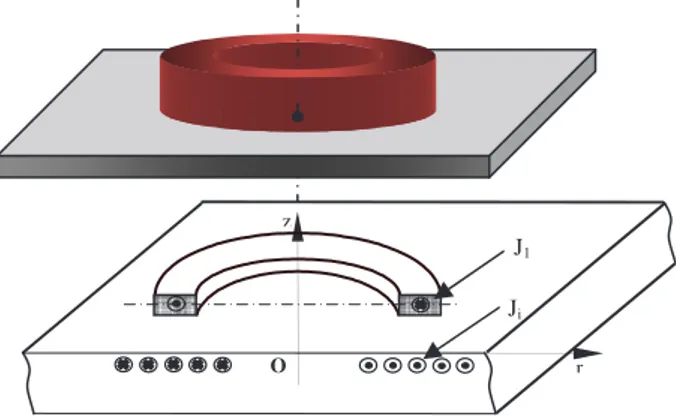
Taking into account that the inductive transducer senses the proximity of a metal body, the model of the transducer consists of a toroidal coil placed parallel to the surface of a conductive flat plate, as shown in Fig. 1.
Fig. 1. Physical model of the inductive proximity transducer
z
O • r
•
J1
The coil is fed with a sinusoidal current with a given r.m.s. value and frequency. Due to the induced currents in the plate, the magnetic flux through the coil changes, varying mainly with the distance coil - plate. We can analyze the dependence of the coil inductance, of its sensitivity and of the voltage at its terminals, function of several parameters, of which the most important is the distance between the coil and the surface of the conductive flat plate, for different variants of the plate material.
B. The electromagnetic field – electrical circuit coupling of the transducer
The physical model of the transducer, as shown in Fig. 1, is characterized by a rotation symmetry and, as a result, the associated field model is 2D axisymmetric, in the cylindrical coordinates (r, z). Coil current density J1 (the source of the electromagnetic field) and the magnetic vector potential A (the unknown state variable of the electromagnetic field) have azimuthal orientation, perpendicular to the rOz plane, Fig. 1. The differential model of the quasi-stationary harmonic electromagnetic field, expressed by the complex image of the magnetic vector potential A, is represented by the equation:
rot[(1/µ)⋅rotA] + jωA/ρ = J1 (1) where ω = 2πf, f is frequency, ρ is the resistivity and µ
is the magnetic permeability. The second term on the left side of the equation represents the induced current density Ji (Fig. 1), non-null only in the plate region, where the electrical conductivity σ = 1/ρ is nonzero.
The current density J1 in the rectangular region in Fig. 1, which represents the axial section through the inductor coil, is the source of the electromagnetic field. The value of this quantity can be quite easily calculated based on transducer geometry data and on power supply data. But it may be considered as an unknown, as the magnetic vector potential, if besides the above equation we take into account the equation of the electric circuit which includes the coil. This circuit includes, on one side, a current source of known intensity I1 and, on the other side, a stranded coil which reflect the field model and at which we know the number of turns, the resistivity of the conductor and the filling factor. As a consequence, the numerical model of the transducer is of the type of electromagnetic field - electric circuit coupling [6].
C. Finite element model of the transducer
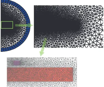
Electromagnetic field computation domain, Fig. 2, which represents half of axial section of the physical model of the transducer, contains the following regions with different physical properties:
- COIL, the region where the current density is denoted by J1. Being made of stranded conductor, there are no induced currents. For this reason, the material associated to this region is non-conductor;
- PLATE, the conductive region in the proximity of the coil, the area of induced currents;
- AIR, the non-conductive and non-magnetic region, which surrounds the inductor-coil and the induced-plate;
- INFINITE, non-conductive and non-magnetic region, which is a transformation of infinite region from outside of the AIR region into a finite region. Using this type of region, we can approach a problem of electromagnetic field, which is usually one with the unlimited expansion.
Fig. 2. Electromagnetic field computation domain
We have considered initially for the metal plate two cases: non-magnetic steel, with ρ=10-6Ωm, respectively
aluminium, with ρ = 0.03⋅10-6 Ωm. The relative
magnetic permeability µr = 1 for entire calculus domain. Coil turns are made by copper, with ρ = 2⋅10-8Ωm.
Construction of the mesh must take into account the areas with intense field and with induced currents. The details of the mesh are illustrated in Fig. 3.
Fig. 3. Particularities of the mesh associated with computation domain
COIL
AIR PLATE
The electrical circuit of the transducer is presented in Fig. 4.
Fig. 4. The electrical circuit model of the transducer
D. The simulations results
Fig. 5,6,7 presents the numerical simulation solutions obtained for different values of input parameters (different plate material, different values of coil-plate distance, denoted with D).
Fig. 5. Electromagnetic field lines in the case of aluminium plate and D = 4 mm
a)
b)
Fig. 6. The chart of magnetic flux density in the case of steel plate and D=14 mm (a), respectively, D=56 mm (b)
a)
b)
Fig. 7. The chart of eddy currents in the plate, in the case of steel plate and D=14 mm (a), respectively, D=56 mm (b)
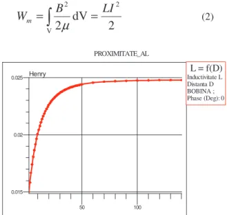
Considering the distance between coil and plate D as a parameter, we can determine the dependence of coil inductance, obtained from numerical model in accordance with eq. (2), function of this distance (Fig. 8)
2
dV
2
2
V 2
LI
B
W
m=
=
µ
(2)PROXIMITATE_AL
0.015 0.02 0.025
50 100
Henry Inductivitate LL = f(D)
Distanta D BOBINA ; Phase (Deg): 0
Fig. 8. The dependence of the inductance of the coil function of the distance to the surface of aluminium plate
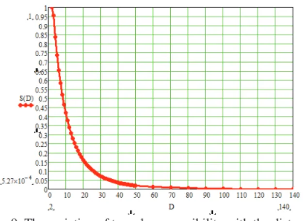
The sensibility of transducer is defined as follows [6]: Sensibility = d(Inductance) / d(D) (3)
Ji[A/mm2]
Ji[A/mm2]
The corresponding dependence of transducer sensibility function of D is illustrated in Fig. 9.
Fig. 9. The variation of transducer sensibility with the distance to the surface of aluminium plate
III. ARTIFICIAL INTELLIGENCE APPROACH Neural Networks (NN) belong to a special group of data analysis techniques that do not resemble with other classical techniques. NN are learning about the chosen subject from the information provided to them, by detecting relationships between input and desired output data, rather than being defined by user [5]
In order to develop and implement a neural network (NN) able to simulate with high fidelity the behavior of the transducer, which can give us the operating parameters of the transducer for any combination of input parameters, first we must create a training database.
We have considered the input parameters as follows:
a) geometry parameters: - the distance coil-metal plate D
- the average diameter of the plate DBMED - the thickness of metal plate GP
b) supply parameters: - frequency F
- r.m.s. value of the coil current – constant value I1 c) material parameter:
- the resistivity of metal plate ROPL The discrete values of parameters are:
D = 2, 3, 4, 5, 6, 7, 8, 9, 10, 12, 14, 16, 18, 20, 25, 30, 35, 40, 45, 50, 60, 70 mm
DBMED = 40, 50, 60, 70, 80, 90 mm GP = 10, 15, 20, 25, 30 mm
F = 400, 750, 1000, 3000, 4000, 7000, 10000 Hz I1 = 0.01, 0.02, 0.03 A
ROPL = 3⋅10-8, 10-7, 10-6 Ωm
Above values gives 41580 possible combinations. Simulations are obtained from an multiparametric solving of numerical model. The computer processor was Intel core 2 duo, 2.13 GHz, 8 GB RAM and the total CPU time was approx. 80 hours.
The database from which we have randomly selected the data sets for training and for testing is a table of values with dimensions 41580x8. The lines number corresponds to all combinations of input parameters and the columns number corresponds to the six parameters and to the two computed quantities, respectively the coil inductance and the voltage at coil terminals.
In order to implement the proposed artificial neural network prediction system the Neural Networks toolbox of the Matlab software package was used
To create a feed-forward network, the following predefined Matlab function was used:
net = newff(P,T,S,TF,PF) (4)
where: P represents the input data vectors; T
represents the target output data vectors; S represents the
number of neurons in each hidden layer; TF represents
the transfer function used for each layer; and PF is
performance function used to evaluate NN provided output data during the training process.
To determine the optimal structure of the proposed neural network, more than 36 feed-forward architectures with two hidden layers and one output layer were tested. The number of neurons on each hidden layer was varied between 5 and 30 with a step of 5 neurons. All created structures are retained in the NNMat array.
Using a custom Matlab function developed by the authors, in the same m-file, at each iteration an NN is created and after that trained in order to produce the desired output data.
net = train(net,InPuts,Targets); (5)
where: net is the artificial neural network created at each
iteration that has to be trained, P is a set of training input
data vectors and T represents the training target output
data vectors.
The transfer functions used are the hyperbolic tangent sigmoid tansig for hidden layers and the the
linear purelin function for the output layer neurons
x x)=
(
purelin (6)
x x
e e x
2 2
1 1 ) (
tansig −
−
+ −
= (7)
The logarithmic sigmoid logsig transfer function
x
e x
−
+ =
1 1 ) (
logsig (8)
did not give the satisfactory results during training process performed on created NN.
It has been used the implicit Levenberg-Marquard training method combined with a descendent gradient with momentum weight backpropagation learning rule.
training stops when one of the convergence criteria is reached.
(
−)
⋅ =
=
n
i
i
i y
y n
e Performanc
1
2 *
1 (9)
where: y* represent the desired output values, y
represents the provided output values of the optimal NN structure, and n represents the number of input/desired
output value pairs used to train the network.
Performance evolution of the identified optimal NN configuration is illustrated in Fig. 10
Fig. 10. The evolution of performance
Next step, having the data set vector NNMat, we must simulate the answer of these NN at other data sets, not used for training, and we will compare their answer with the numerical results obtained from FEM analysis.
For the simulation, another predefined Matlab function was used
sim(NN,InPutData) (10)
The neural network selected in order to models the mathematical function that offers the values of coil inductance L for any combination of input parameters has 30 neurons on the first hidden layer and 30 neurons on the second hidden layer. This structure offers a very high precision in finding the inductance L, the average relative error being of only 0.885 %. Analyzing the behavior of this NN for all data sets, it can be observed an maximum relative error of 4.52 %, for a single data set, all the others data sets resulting in errors in range 0.1...2.5 %.
Other acceptable structures for the searched neural network are:
- network with 15 neurons on first hidden layer and 30 neurons on the second layer, that give an average relative error of 0.904 %
- network with 5 neurons on first hidden layer and 10 neurons on the second layer, that give an average relative error of 0.940 %.
Furthermore, it was done a detailed analysis on operating mode predictions of inductive proximity transducer using the selected neural network, respectively an NN feed-forward backpropagation error type, with 2 hidden layers, with 30 neurons on first and 30 neurons on second hidden layer.
It was studied the dependence of total inductance of transducer coil function of the most relevant input parameter, respectively the distance coil-metal plate, in the case of fixed values for all other parameters. We considered these values as follows:
- the resistivity of metal plate: ROPL = 3⋅10-8 Ωm
(aluminium);
- the thickness of plate: GP = 20 mm (approx. 5 times greater than the skin depth of eddy currents induced in the plate);
- the average diameter of the coil: DBMED = 70 mm; - r.m.s. value of the current through the coil turns: I1=0.01 A
- frequency of power supply: F = 400 Hz
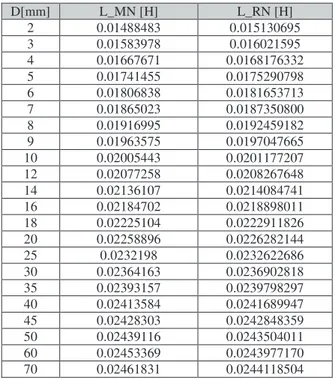
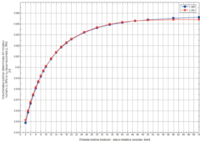
The comparison between the values of coil inductance obtained in two ways, based on the simulations using the finite element model built in chapter II and based on simulations using the selected neural network, is illustrated in Table 1 and Fig. 11. Table 1. Coil inductance values obtained based on simulations using FEM model (L_MN) and based on simulations using the selected NN (L_RN)
D[mm] L_MN [H] L_RN [H]
2 0.01488483 0.015130695
3 0.01583978 0.016021595
4 0.01667671 0.0168176332
5 0.01741455 0.0175290798
6 0.01806838 0.0181653713
7 0.01865023 0.0187350800
8 0.01916995 0.0192459182
9 0.01963575 0.0197047665
10 0.02005443 0.0201177207
12 0.02077258 0.0208267648
14 0.02136107 0.0214084741
16 0.02184702 0.0218898011
18 0.02225104 0.0222911826
20 0.02258896 0.0226282144
25 0.0232198 0.0232622686
30 0.02364163 0.0236902818
35 0.02393157 0.0239798297
40 0.02413584 0.0241689947
45 0.02428303 0.0242848359
50 0.02439116 0.0243504011
60 0.02453369 0.0243977170
70 0.02461831 0.0244118504
Fig. 11. The dependence of coil inductance on the distance between coil and metal plate, obtained in the two ways: based
on simulations using FEM model (L_MN) and based on simulations using the selected neural network (L_RN).
IV. CONCLUSIONS
Comparing the results of numerical experiments based on FEM model with simulations results using NN, we have registered the average errors of approx. 2% for followed output quantity, respectively the inductance of the transducer coil. The results fully justify the method discussed, taking into account in addition the much lower computational effort.
REFERENCES
[1] Simon Hykin, Neural Networks and Learning Machines,
Third Edition, Prentice Hall, 2009
[2] Virgil Tiponut, Catalin Daniel Caleanu, Neural networks. Architectures and algorithms (in Romanian), Ed. Politehnica Timisoara, 2002
[3] Levente Czumbil, Dan D. Micu, Francisc I. Hathazi, “Operating Mode Prediction of a Microwave Heating System using Artificial Intelligence Techniques”, The 8th International Symposium on Advanced Topics in Electrical Engineering ATEE 2013, Bucharest, 2013
[4] D.D. Micu, L. Czumbil, A. Ceclan, E. Simion, Denisa Ste , Liliana Cîmpan, “Neural Network Evaluation of Electromagnetic Interferences between HV Power Lines and Underground Metallic Pipelines”, Proceedings of the 11th International Conference on Engineering of Modern Electric Systems, EMES’09, Oradea, 2009
[5] D.D. Micu, L. Czumbil, G.C. Christoforidis, and E. Simion, “Neural Networks Applied in Electromagnetic Interference Problems”, Rev. Roum. Sci. Techn.– Électrotechn. et Énerg., vol. 57, no. 2, pp. 162-171, 2012 [6] Virgiliu Fireteanu, Monica Popa, Tiberiu Tudorache,
Numerical models in the study and design of electromagnetic devices (in Romanian), Ed. MatrixRom, Bucharest, 2000
[7] C. I. Mocanu, Electromagnetic field theory (in Romanian), Ed. didactica si pedagogica, Bucharest, 1980 [8] G. Mindru, M. Radulescu, Numerical analysis of the
electromagnetic field (in Romanian), Ed. Dacia,
Cluj-Napoca, 1986