www.atmos-chem-phys.net/11/10389/2011/ doi:10.5194/acp-11-10389-2011
© Author(s) 2011. CC Attribution 3.0 License.
Chemistry
and Physics
Simulating deep convection with a shallow convection scheme
C. Hohenegger1,*and C. S. Bretherton1
1Department of Atmospheric Sciences, University of Washington, Seattle, WA, USA *now at: Max Planck Institute for Meteorology, Hamburg, Germany
Received: 10 December 2010 – Published in Atmos. Chem. Phys. Discuss.: 11 March 2011 Revised: 11 July 2011 – Accepted: 7 October 2011 – Published: 19 October 2011
Abstract.Convective processes profoundly affect the global water and energy balance of our planet but remain a chal-lenge for global climate modeling. Here we develop and investigate the suitability of a unified convection scheme, capable of handling both shallow and deep convection, to simulate cases of tropical oceanic convection, mid-latitude continental convection, and maritime shallow convection. To that aim, we employ large-eddy simulations (LES) as a benchmark to test and refine a unified convection scheme implemented in the Single-column Community Atmosphere Model (SCAM). Our approach is motivated by previous cloud-resolving modeling studies, which have documented the gradual transition between shallow and deep convection and its possible importance for the simulated precipitation diurnal cycle.
Analysis of the LES reveals that differences between shal-low and deep convection, regarding cloud-base properties as well as entrainment/detrainment rates, can be related to the evaporation of precipitation. Parameterizing such effects and accordingly modifying the University of Washington shallow convection scheme, it is found that the new unified scheme can represent both shallow and deep convection as well as tropical and mid-latitude continental convection. Compared to the default SCAM version, the new scheme especially im-proves relative humidity, cloud cover and mass flux profiles. The new unified scheme also removes the well-known too early onset and peak of convective precipitation over mid-latitude continental areas.
Correspondence to:C. Hohenegger ([email protected])
1 Introduction
Accurate representation of deep convection with global cli-mate models of coarse resolution remains a nagging problem for the simulation of present-day and future climates. Typical biases include the simulation of a double Inter-Tropical Con-vergence Zone (ITCZ, see e.g., Bretherton, 2007; Lin, 2007), a too weak, too fast or spatially distorted Madden-Julian Oscillation (MJO, see e.g., Slingo et al., 1996; Bretherton, 2007) and poor timing of convection with a too early onset, peak and decay of precipitation. This last bias is apparent both over the Tropics (e.g., Yang and Slingo, 2001; Bech-told et al., 2004) and mid-latitude continental areas (e.g., Dai et al., 1999; Lee et al., 2007).
Many approaches have been proposed over the years to pa-rameterize deep convection (see e.g., Arakawa, 2004; Ran-dall et al., 2003, for a review). The most popular method remains the use of a mass flux scheme (see e.g., Plant, 2010; Arakawa and Schubert, 1974). The latter aims to predict the vertical structure and evolution of a one-dimensional entraining-detraining plume (bulk mass flux scheme) or spectrum thereof (spectral mass flux scheme). Irrespective of the specific design, convection schemes have to rely on some assumptions to relate the sub-scale cloud behavior to the large-scale resolved flow. Such relations are hard to get from observations and hard to formulate.
Atmosphere Coupled Ocean Atmosphere Response Exper-iment (TOGA COARE) and found good agreement with cloud-resolving model simulations. Several studies also doc-umented improvements in tropical convection, without nev-ertheless being able to fully remove the ITCZ or MJO bi-ases, by employing more elaborate entrainment/detrainment formulations (e.g., Chikira and Sugiyama, 2010; Bechtold et al., 2008; Li et al., 2007; Wang et al., 2007), revised clo-sures/triggering functions (e.g., Deng and Wu, 2010; Li et al., 2007; Zhang and Mu, 2005; Neale et al., 2008) or by introducing convective momentum transport (e.g., Deng and Wu, 2010; Richter and Rasch, 2008). The possible impacts of such modifications are in general strongly model dependent and confined to certain aspects of the simulated convection. In this respect it is still not clear whether a single convec-tive parameterization can realistically handle both tropical oceanic and mid-latitude continental convection.
This study is geared towards improving the simulation of deep convection in coarse-resolution climate models. In con-trast to the approach employed in most such models, we seek to develop a unified convection scheme starting from a pa-rameterization designed for shallow cumulus convection. We regard shallow convection as mostly non-precipitating con-vection with no ice formation. Deep concon-vection will refer to precipitating convection. Cloud-resolving modeling stud-ies have documented the gradual transition occurring from shallow to deep convection and highlighted its importance for the simulated convective diurnal cycle (e.g., Guichard et al., 2004). This may be best achieved with a unified scheme. Our study is a step in this sense. We will explore how to unify shallow and deep convection and present single-column model experiments to test our results.
The basic hypothesis behind our approach is that the main difference between shallow and deep convection is precipi-tation (both rain and snow) and its effects. Evaporation of precipitation (hereafter called rain evaporation) modifies the atmospheric environment and especially the structure of the planetary boundary layer (PBL), which feeds back on the convective development. Including such effects in a shal-low convection scheme should thus alshal-low the representation of deep convection within the same scheme. We thus see deep convection as highly interactive with the PBL state, like shallow convection. Our parameterization approach is further motivated by the results of recent large-eddy simu-lations (e.g., Khairoutdinov and Randall, 2006) which have highlighted the importance of rain evaporation for deep con-vection.
In order to fulfill our goals and test our hypothesis, we will employ large-eddy simulations of different convective events. We will investigate modifications in the PBL struc-ture and in the atmospheric environment due to falling pre-cipitation, and derive appropriate relations to describe them. These relations will then be implemented in the shallow con-vection scheme developed at the University of Washington (UW) by Bretherton et al. (2004) and Park and Bretherton
(2009). Using a single-column version of the National Center for Atmospheric Research (NCAR) Community Atmosphere Model (CAM), the performance of the new unified scheme will be assessed against large-eddy simulations, the default version of the CAM single-column model, and a version of the single-column model in which the UW shallow convec-tion scheme is used without modificaconvec-tion (but also without any separate deep convection scheme).
As this paper was being written, Mapes and Neale (2011) also presented results of CAM simulations with a unified convection scheme. They extended the UW shallow con-vection scheme to a two plume model and introduced a new prognostic variable called org to control the transition be-tween shallow and deep convection.orgis meant to represent convective organization and acts upon cloud-base properties and lateral mixing rates. The source oforgis rain evapora-tion with an arbitrary set conversion rate. Our approach bears similarities with the one of Mapes and Neale (2011) as it also uses rain evaporation and its effects on cloud-base proper-ties and mixing rates to control the transition from shallow to deep convection. However we stick to the one plume model, do not introduce new prognostic equations and employ large-eddy simulations to quantify the effect of rain evaporation on the subsequent cloud development.
The outline is as follows. Section 2 presents our method with a description of the different models, cases considered, and our experimental set-up. Section 3 focuses on the plan-etary boundary layer; changes in cloud-base mass flux and cloud-base thermodynamic properties between shallow and deep convection are investigated, parameterized and tested with single-column model experiments. Section 4 repeats the analysis for entrainment and detrainment rates. Conclusions are given in Sect. 5.
2 Method
2.1 Models
The large-eddy simulations (LES) are performed with the System for Atmospheric Modeling (SAM, see Khairoutdi-nov and Randall, 2003). The model solves the 3D anelas-tic equations given prescribed large-scale tendencies and sur-face fluxes/sea sursur-face temperature. As parameterization, the model includes a bulk microphysics scheme, a Smagorinsky-type scheme to represent subgrid-scale turbulence, and the radiation package (Collins et al., 2006) taken from the NCAR CAM3 global climate model (GCM). A more detailed de-scription of SAM can be found in Khairoutdinov and Randall (2003).
of CAM3 (see Collins et al., 2006) with a modified treat-ment of deep convective motreat-mentum transport (Richter and Rasch, 2008) and a revised deep convective trigger (Neale et al., 2008). CAM3 includes a surface-driven boundary-layer turbulence scheme based on Holtslag and Boville (1993). Deep convection is parameterized after Zhang and McFar-lane (1995) while shallow convection follows Hack (1994). As alternate parameterizations, the model can be run with new moist turbulence and shallow convection schemes devel-oped at the UW (see Bretherton and Park, 2009; Bretherton et al., 2004; Park and Bretherton, 2009).
2.2 The UW shallow convection scheme
Since the UW shallow convection scheme serves as the start-ing point to develop a unified convection scheme, it is ex-plained here in more detail. It is a mass flux scheme based on a buoyancy-sorting, entrainment-detrainment plume model. Updraft mass fluxMu and updraft propertiesψu are
com-puted according to:
∂Mu
∂z =Mu(ǫ−δ) (1)
∂ψu
∂z =ǫ(ψ−ψu)+Sψ (2)
withǫ the fractional entrainment rate, δ the fractional de-trainment rate,ψ the mean environmental property andSψ
source term. The mass flux at cloud baseMcbis determined
by the ratio between convective inhibition (CIN) and mean planetary boundary layer turbulent kinetic energy (TKE):
Mcb=0.4ρ
p
TKEexp(−CIN
TKE) (3)
withρthe air density. CIN is implicitly computed within the scheme (see Park and Bretherton, 2009), while TKE must be provided by the boundary layer scheme. This ensures tight interactions between the planetary boundary layer (PBL) and cumulus convection. If the lifting condensation level (LCL) is much higher than the top of the boundary layer, CIN is very large and air parcels don’t have enough kinetic energy to overcome their CIN. The boundary layer height increases via entrainment until it reaches the LCL. As a result, CIN decreases, the mass flux increases and compensating subsi-dence increases preventing the PBL to rise further. The clo-sure thus acts to keep the cumulus base near the top of the PBL and keeps CIN on the same order as TKE (Fletcher and Bretherton, 2010).
Cloud properties are expressed in terms of the total water mixing ratioqt=qv+ql+qiand the ice-liquid water
poten-tial temperatureθli=θ−qlLv/5cp−qiLf/5cp(Deardorff,
1976), withθthe potential temperature,qi,qlandqvthe ice,
liquid water and water vapor mixing ratios,LvandLfthe
la-tent heat of vaporization and of sublimation,cp the specific
heat of dry air at constant pressure, and5the Exner pressure function. Both qt and θli are assumed to be conserved for
non-precipitating moist adiabatic processes. At cloud base,
qt is set to its surface value, whileθli is diagnosed from the
lowest value of the virtual potential temperature over the PBL and the value ofqtat cloud base. Updraft vertical velocitywu
is diagnosed solving 1
2
∂ ∂zw
2
u=aBu−bǫwu2 (4)
withBu updraft buoyancy,a virtual mass coefficient and b
drag coefficient.aandbare set to 1 and 2, respectively (see Bretherton et al., 2004, for more detail). The updraft verti-cal velocity determines the maximum height reached by the plume.
Entrainment and detrainment processes are parameterized using buoyancy sorting principles. Mixing of cloudy air with environmental air generates a spectrum of mixtures with dif-ferent buoyancies and vertical velocities. It is assumed that only mixtures that can travel a certain vertical distancelcrit
remain in the updraft. By assuming that the generated spec-trum of mixtures is uniform, the fractional entrainment and detrainment rates per unit height are found to be
ǫ=ǫ0χc2 (5a)
δ=ǫ0(1−χc)2 (5b)
The critical mixing fractionχc depends on height; at each
level it is fully determined by the chosenlcrit as well as by
the updraft and environmental properties expressed by their buoyancy and humidity (see Eq. (B1) in Bretherton et al., 2004). The fractional mixing rateǫ0(m−1) is set empirically
to 8/z, withz(m) being the height above ground. The scheme also includes enhanced penetrative entrainment above the level of neutral buoyancy of the bulk updraft (see Eq. (D1) in Bretherton et al., 2004).
The UW shallow convection scheme employs extremely simple microphysics: condensate larger than 1 g kg−1is
re-moved from the updraft as precipitation, which is partitioned between a fixed fraction that can fall through the updraft (and which can only evaporate below the cumulus base) and a re-mainder that is detrained into the environment (and which can evaporate above cloud base). In either case, the evapora-tion rate depends upon the saturaevapora-tion deficit and the precipi-tation flux. Note that while rain evaporation drives organized downdrafts in reality, there is no explicit downdraft formula-tion in the scheme; evaporated precipitaformula-tion homogeneously cools the entire grid cell.
controlling the cloud development. Those are thus the three quantities that we will examine in more detail in Sects. 3 and 4 and modify with appropriate relationships to design a uni-fied convection scheme.
2.3 Cases
In order to investigate issues related to the parameteriza-tion of moist convecparameteriza-tion, we consider three cases that have been well observed and extensively studied in the past. They have been chosen to span diverse atmospheric conditions and types of convection.
The first case is taken from measurements made at the At-mospheric Radiation Measurement (ARM) Southern Great Plains station between 19 June and 3 July 1997 (Julian days 170–186). This case typifies continental summertime mid-latitude convection. The period encompasses a wide range of conditions, including clear days, shallow convection, di-urnally forced convection, and precipitation associated with the passage of extratropical cyclones and fronts.
The second case represents tropical marine deep convec-tion. The measurements are taken from the Kwajalein Ex-periment (KWAJEX) over the west Pacific warm pool. We restrict here our analysis to the period 24 July–10 September 1999 (Julian days 205–253).
Finally, we also consider the Barbados Oceanographic and Meteorological Experiment (BOMEX), a frequently simu-lated example of non-precipitating shallow trade-cumulus convection. The forcing data are derived from observations taken on 22–23 June 1969.
2.4 Experimental set-up
The three cases are simulated with SAM and with different versions of SCAM, using prescribed time-dependent profiles of large-scale vertical motion and horizontal advective heat-ing and moistenheat-ing as well as surface fluxes (for ARM) and sea surface temperature (for KWAJEX and BOMEX). Each SAM simulation is doubly periodic in the horizontal but em-ploys a different grid. For the ARM case, SAM is run with a horizontal resolution of 500 m with 384×384 grid points
and 96 vertical levels going up to 30 km. The grid spacing varies between 50 m near the surface to 250 m in the mid-troposphere. The KWAJEX simulation has a horizontal res-olution of 1000 m and a vertical resres-olution of 100 m near the surface up to 400 m in the mid-troposphere. The domain con-tains 256×256×64 grid points. For both ARM and KWA-JEX, the domain-mean winds are nudged to the time-varying observational profiles with a one-hour relaxation time. Fi-nally, the BOMEX simulation contains 256×256×96 grid points with a resolution (both horizontally and vertically) of 40 m. In the upper third of the domain, perturbations to the horizontal mean are linearly damped to help absorb convectively-forced gravity waves. For BOMEX, the winds
are forced by a geostrophic wind profile rather than through nudging.
Similar simulations of SAM have been validated and in-vestigated in detail by Khairoutdinov and Randall (2003) for ARM, Blossey et al. (2007) for KWAJEX, and Siebesma et al. (2003) for BOMEX. These studies show that the SAM model reproduces the overall convective development fairly accurately compared to observations in all three cases. Hence, we will use the SAM simulations as a benchmark both to characterize the behavior of the cumulus ensemble and to validate the SCAM single-column model experiments. For all cases, SCAM is run with 30 vertical levels and a time step of 5 min, driven by the same large-scale forc-ing and surface fluxes/sea surface temperature as SAM. For KWAJEX and BOMEX, the start and end times of the SCAM simulations coincide with the SAM integrations. For ARM, only specific rain events are simulated with SCAM instead of the full time period as a whole. This is to ensure that differences obtained between the integrations are due to the convective parameterization rather than to the simulation of different atmospheric conditions. Indeed, SCAM drifts away from SAM with time in ARM due mainly to different timings and amplitudes of individual rain events. For each rain event, we employ the SAM-simulated mean profiles as initial data for the SCAM simulations. The specific events that we sim-ulate (see, e.g. Fig. 1) are days 174 (05:30 UTC Julian day (JD) 174 to 11:30 UTC JD 175), 176 (05:30 UTC JD 176– 11:30 UTC JD 177), 178 (05:30 UTC JD 178–05:30 UTC JD 179), 179 (05:30 UTC JD 179–05:30 UTC JD 180) and 180 (05:30 UTC JD 180–11:30 UTC JD 181). Days with strong large-scale forcing are omitted since SCAM will tend to per-form well for those cases due to the use of prescribed large-scale tendencies.
To investigate the performance of the new unified con-vection scheme, three main types of SCAM simulations are performed (Table 1). The first experiment employs the de-fault version of the CAM3.5 model, in which PBL processes are parameterized after Holtslag and Boville (1993), shal-low convection after Hack (1994) and deep convection af-ter Zhang and McFarlane (1995). This simulation is called CAM and serves as our control experiment.
The second experiment employs the UW PBL scheme, the UW shallow convection scheme and no deep convective pa-rameterization. In this case, precipitation associated with deep convection will only be produced if the full grid cell reaches saturation (through SCAM microphysical scheme) or if the shallow convection scheme by itself succeeds in pro-ducing deep plumes. It can thus be expected that this simu-lation will underestimate deep convection. The experiment is called UWS and is otherwise identical to the CAM exper-iment.
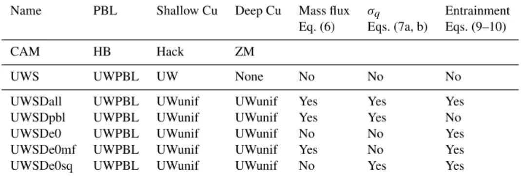
Table 1.Overview of the different SCAM simulations. HB stands for Holtslag and Boville (1993), Hack for Hack (1994), ZM for Zhang and McFarlane (1995), UWPBL for the University of Washington PBL scheme (Bretherton and Park, 2009) and UW for the default University of Washington shallow convection scheme (Park and Bretherton, 2009). UWunif corresponds to the new unified convection scheme.
Name PBL Shallow Cu Deep Cu Mass flux σq Entrainment
Eq. (6) Eqs. (7a, b) Eqs. (9–10)
CAM HB Hack ZM
UWS UWPBL UW None No No No
UWSDall UWPBL UWunif UWunif Yes Yes Yes
UWSDpbl UWPBL UWunif UWunif Yes Yes No
UWSDe0 UWPBL UWunif UWunif No No Yes
UWSDe0mf UWPBL UWunif UWunif Yes No Yes
UWSDe0sq UWPBL UWunif UWunif No Yes Yes
Fig. 1. Time series of precipitation at cloud base; black curve for onset and mature precipitation phase, grey for decay phase, and tur-bulent kinetic energy averaged over the planetary boundary layer; red curve for onset and mature phase; orange for decay phase, for (a)ARM and(b)KWAJEX.
are identical in their set-up to CAM and UWS. They are called UWSDpbl, UWSDall, UWSDe0, UWSDe0mf and UWSDe0sq, depending on the modifications made to the UW shallow convection scheme. The modifications are de-scribed along the text and in Table 1. Ideally, those simula-tions should stand in closer agreement to SAM than both the CAM and the UWS integrations.
3 The planetary boundary layer under deep convection
As stated in the introduction, we regard deep convection as shallow convection modified due to its production of heavy precipitation. In this view, the cloud-base mass flux in deep as well as shallow convection is regulated by the PBL and
the subcloud mixed layer. Bulk instability measures like con-vective available potential energy (CAPE) are relevant to the vertical structure of cumulus convection, which in turn indi-rectly modifies the thermodynamic structure of the PBL and the overlying air. However, they are not viewed as direct controls on the cloud-base mass flux. This approach is sup-ported by Kuang and Bretherton (2006), who showed that changes in CIN and TKE were closely correlated in large-eddy simulations of an idealized transition from shallow to deep convection and Fletcher and Bretherton (2010), who showed that a closure based on CIN and TKE could pre-dict the cloud-base mass flux in LES simulations of ARM, KWAJEX and BOMEX. We especially refer to the study of Fletcher and Bretherton (2010) for more details on the ad-vantages/disadvantages of employing a closure based on CIN and TKE. We nevertheless note that such a closure allows for a more straightforward implementation of precipitation effects on the cloud-base mass flux than a closure based on CAPE.
In this section, we thus investigate how changes in the PBL structure between shallow and deep convection, espe-cially due to rain evaporation, affect cloud-base mass flux and cloud-base thermodynamic properties. Both are key pa-rameters controlling the convective development. We use the SAM outputs to derive appropriate relations characterizing such effects. Except noted otherwise, all the quantities are computed from the SAM output statistics. The latter are computed at each time step and averaged both horizontally (if appropriate) and over one hour time interval. The derived relations are then implemented in the UW shallow convec-tion scheme and tested in a single-column mode.
3.1 SAM results
3.1.1 Cloud-base mass flux
Figure 1 shows the time series of TKE and precipitation at cloud baseRRcb for ARM and KWAJEX obtained from
0 0.5 1 1.5
x 10−3 0
5 10 15 20 25 30
RR
cb*PBLH [m 2s−1]
TKE [m
2s
−2
]
0 0.2 0.4 0.6 0.8 1
x 10−3 0
5 10 15 20
RR
cb*PBLH [m 2s−1]
TKE [m
2s
−2
]
a) ARM b) KWAJEX
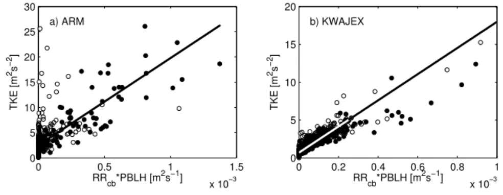
Fig. 2.Scatter plots of TKE versusRRcb·PBLH based on hourly statistics from(a)ARM and(b)KWAJEX. Full circles are for onset and mature precipitation phase, open circles for the decay phase. Onset, mature and decay phases are distinguished in Fig. 1. Slope of the solid regression line in(a)and(b)is 17 280 s−1. There are 125 (530) and 285 (639) points in ARM (KWAJEX) for the onset/mature and decay phase, respectively.
horizontally averaged fields). TKE is averaged over the depth of the planetary boundary layer PBLH and is denoted here-after TKE. PBLH is diagnosed as the height where the resolved-scale turbulent buoyancy flux reaches its minimum. The cloud base is defined following Fletcher and Brether-ton (2010) as the lifting condensation level of an air parcel with a potential temperature equal to the potential tempera-ture averaged over the layer 200–400-m and a water vapor mixing ratioqvequal to the mean 200–400-mqv+σq, where σq is the horizontal standard deviation inqv averaged over
the same height range. If the estimated cloud base is lower than the PBL height, we set its value to the height of the PBL, as done in the UW scheme.
It is evident in Fig. 1 that TKE increases from shallow to deep convection, i.e. with increasing precipitation. This in-crease is driven by rain evaporation, which generates cold pools that induce horizontal flows. Together with the associ-ated organized surface convergence along cold pool bound-aries, it represents a supplementary energy source for lifting an air parcel and thus favors the development of convection, as is apparent in our SAM simulations and many past studies of deep convection (see e.g., Rio et al., 2009; Khairoutdinov and Randall, 2006).
The increase in TKE due to cold pool activity is not di-rectly resolved by a coarse-resolution global model. Rio et al. (2009) represented this effect by implementing a density current parameterization and coupling it to Emanuel (1991)’s scheme. Here we follow a simpler, more empirical, approach to parameterize this effect.
Figure 2 shows a scatter plot of TKE versus a measure of evaporative potential (and thus cold pool activity) formed as the product ofRRcband PBLH, for our ARM and KWAJEX
simulations. The full circles in Fig. 2 are for the onset/mature phase in which shallow convection is developing into deep precipitating convection, while open circles are for the decay phase. The times classified into the different phases, subjec-tively determined from the domain-mean precipitation time
series, are indicated in Fig. 1 for reference.
Figure 2 indicates that TKE scales withRRcb·PBLH with
a similar slope both for KWAJEX and ARM. The value for zero precipitation should correspond to the TKE in a dry con-vective boundary layer TKEdry, which is predicted by the
PBL scheme. We can thus write:
TKE=TKEdry+C·RRcb·PBLH (6)
with C=17280 s−1, RRcb in m s−1, TKE in m2s−2 and
PBLH in m. The correlation coefficient is 0.92 for KWA-JEX and 0.83 for ARM during the onset/mature phase. The correlation is quite strong: adding further predictors does not provide any additional skill. The larger scatter in ARM re-sults from the larger variability in the sampled synoptic con-ditions. The agreement worsens during the decay precipi-tation phase as cold pools need time to dissipate after rain evaporation is finished.
The evaporation of convective precipitation induces a pos-itive feedback between convection and boundary-layer pro-cesses embodied in Eq. (6), because it generates TKE that yields more convection and more precipitation. However, rain evaporation also cools and stabilizes the PBL. At a cer-tain point, the PBL collapses and shuts down convection. This effect is expressed by the use of PBLH in Eq. (6). 3.1.2 Cloud-base thermodynamic properties
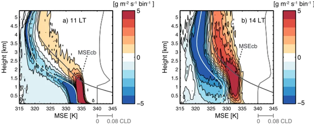
Figure 3 shows example profiles of mass flux as a function of moist static energy (MSE) for ARM day 178 at 11:00 and 14:00 LT. In contrary to the other Figures, we employ the instantaneous 3D output from SAM to construct Fig. 3. 11:00 LT corresponds to the shallow convection phase, while 14:00 LT illustrates the situation under deep convection.
MSE [K]
Height [km]
315 320 325 330 335 340 345
0.5 1 1.5 2 2.5 3 3.5 4 4.5 5
−5 0 5
MSE [K]
Height [km]
315 320 325 330 335 340 345
0.5 1 1.5 2 2.5 3 3.5 4 4.5 5
−5 0 5
a) 11 LT b) 14 LT
[g m-2 s-1 bin-1 ] [g m-2 s-1 bin-1 ]
0 0.08 CLD 0 0.08 CLD
MSEcb MSEcb
Fig. 3. Profiles of mass flux as a function of MSE for ARM day 178 at(a)11:00 and(b)14:00 LT (local time). White and black lines represent domain-averaged MSE (K) and saturation MSE (K). Grey line indicates the profile of cloud fraction (CLD), while the dashed arrow indicates MSEcb.
is exact (except for ice processes) given the thermody-namic equations employed in SAM. Throughout this pa-per, MSE is rescaled into temperature units by dividing by
cp=1006 J kg−1K−1.
The profiles in Fig. 3 are obtained by binning at each height the grid points by their MSE and summing their mass flux per bin (see Kuang and Bretherton, 2006). The bin size is 0.25 K. Light to dark red colors in Fig. 3 im-ply positive values of the vertical velocity and thus repre-sent updrafts, while light to dark blue colors reprerepre-sent down-drafts/subsidence. Figure 3 also displays in white and black the domain-averaged MSE and the domain-averaged satu-rated MSE, as well as the domain-averaged cloud cover in grey. Equivalently, the shaded portion in Fig. 3 above the black line of the saturated MSE can be interpreted as repre-senting the cloudy points.
Comparison of Fig. 3a and b reveals similarities and dif-ferences in the partitioning of cloud-base MSE between shal-low and deep convective updrafts and downdrafts. The cu-mulus cloud base is visible in both plots as the altitude of maximum lower-tropospheric cloud fraction; at this level the mean updraft MSE, indicated by MSEcbin Fig. 3, is almost
identical to the domain-mean saturation MSE at that height, suggesting the cumulus updrafts have nearly the same tem-perature (and hence buoyancy) as their environment at cloud base. Above cloud base, the net upward mass flux is car-ried almost exclusively within cumulus clouds. Since clouds are less numerous than cloud-free grid points the line of the domain-mean MSE does not pass in-between up- and down-drafts but is shifted towards the environment. The typical range of MSE carried by the upward mass flux is also verti-cally continuous across cloud base at both times.
Before strong precipitation (Fig. 3a), the PBL has a struc-ture akin to the strucstruc-ture of a dry convective boundary layer. Half of the PBL experiences updrafts with slightly higher MSE, half downdrafts with slightly lower MSE and MSEcb,
as originating from the warmer part of the MSE spectrum, appears slightly warmer than the values of the domain-mean MSE in the PBL (the white line). Later on (Fig. 3b), precipitation-driven downdrafts bring a broad range of lower MSE into the PBL. Only the remaining high-MSE part of the PBL contributes to the convective cloud-base updrafts, and the difference between MSEcband the values of the
domain-mean MSE in the PBL (the white line) increases.
We find that for both shallow and deep convection, the mean updraft MSE at cloud base MSEcbcan be
parameter-ized as follows (using SAM domain- and hourly-averaged statistics):
MSEcb=MSE+(L/cp)σq (7a)
σq=1×10⁻³(0.45+0.035min(RRcb,20)) (7b)
withRRcbgiven in mm day−1, MSE defined as the MSE
av-eraged over the vertical layer 200–400 m,σq the horizontal
standard deviation in specific humidity averaged over that same vertical layer andL=2.5×10⁶J kg−1.
The expression in Eq. (7a) is inspired by Fletcher and Bretherton (2010), who, through trial and error, found it the most skillful at predicting cloud-base properties (see their Sect. 3a). Equation (7b) contains the approximation to com-puteσq. It is obtained by fitting a first-order polynomial in
RRcb toσq. RRcb is chosen as the predictor since the
in-creased PBL variability is mainly due to cold pool formation. Note that, even without precipitation, Eq. (7a) will predict a small increase in MSEcb. This is consistent with Fig. 3a and
with the presence of turbulent eddies under shallow convec-tion. Equation (7b) also sets an upper bound onσqto express
the fact that the pool of warm air available for updraft forma-tion is limited, especially when cold pools begin to fill up the boundary layer.
5 10 15 20 25 30 35 40 45 50 0
0.2 0.4 0.6 0.8 1 1.2 1.4 1.6 1.8
2x 10 −3
RR cb [mm day
−1] σq
KWAJEX
ARM
BOMEX
Fig. 4. Scatter plot of σq versus precipitation at cloud base for KWAJEX (full circles, 1169 points), ARM (open circles, 410 points) and BOMEX (blue cross, 1 point) based on hourly statis-tics. The red line denotes the fit through the points (see Eq. 7b).
to capture the overall values ofσqfor KWAJEX and ARM.
As a numerical example, MSEcbis larger than MSE by about
1 K on Fig. 3a, which matches the value of(L/cp)σq
pre-dicted by Eq. (7b) assuming no precipitation. The large spread by small precipitation amount, especially in ARM, is due to points from the decay phase where cold pools need time to dissipate. On the other hand, Eq. (7b) will overesti-mateσqand MSEcbin BOMEX. Since this does not seem to
negatively impact our results (see Sect. 4.2), use of a more complicated expression forσqseems unwarranted.
3.2 SCAM experiments
We now use the results of Sect. 3.1 to modify cloud-base characteristics of the UW shallow convection scheme to help make it more suitable for deep convection. The new simu-lation is called UWSDpbl. In contrast to UWS, it employs the mass flux closure developed by Fletcher and Bretherton (2010) based on the same set of LES simulations as we use. This closure, like the default UW shallow cumulus mass flux closure, relates the mass flux to an exponential function of the ratio between CIN and TKE, but multiplies this function by a different prefactor. The closure reads:
Mcb=0.06ρwcbexp(−CIN/TKE) (8a) wcb=0.28
p
TKE+0.64 (8b)
withMcbmass flux at cloud base andwcbvelocity at cloud
base. As an addition, UWSDpbl employs Eq. (6) to predict the cold pool contribution augmenting TKE in the mass flux closure Eqs. (8a)–(8b). The augmentation is done in the
con-vection scheme, but similar results can be obtained by in-creasing TKE in the boundary layer scheme. This is because of the tight coupling existing between the two schemes when employing a CIN/TKE closure, as noted in Sect. 2.2. In UWS, TKE simply equals TKEdry, which is provided by the
UW boundary layer scheme.
Cloud-base thermodynamic properties are expressed in UWSDpbl as the mean over the 200–400 m layer plus one standard deviation in humidity σq (see Eq. 7a), instead of
their surface or minimum values in UWS (see Sect. 2.2).σq
is predicted with Eq. (7b). Finally, the proportionality con-stant scaling the evaporation rate of falling precipitation is increased from 2×10⁻⁶to 1.5×10⁻⁵to be consistent with
the values obtained from the SAM simulations (not shown). It is important to note that the modifications in TKE and cloud-base thermodynamical properties introduced in UWS-Dpbl require PBLH andRRcbas predictors. PBLH is passed
over from the boundary layer scheme. ForRRcbwe employ
the precipitation averaged over the last hour to avoid unde-sirable effects associated with the on-off nature of convection schemes. The precipitation update also occurs at the end of the convection scheme and not in an iterative way. This pre-vents the scheme from adjusting within the loop rather than with time when transitioning from shallow to deep convec-tion.
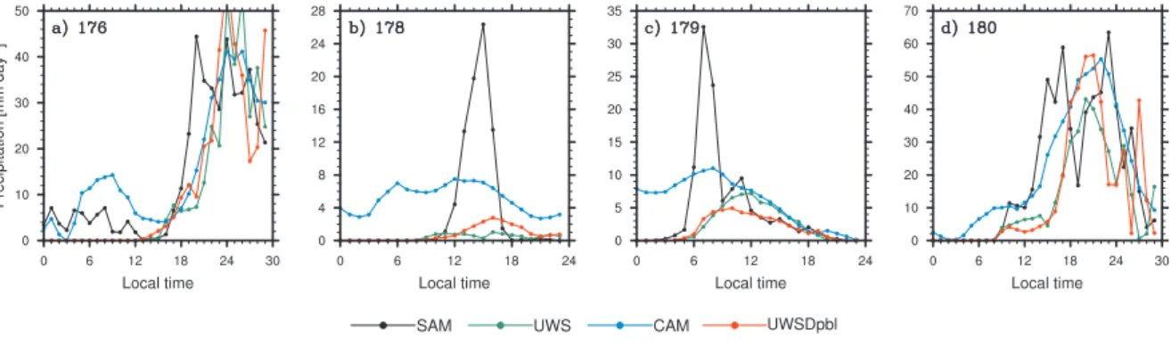
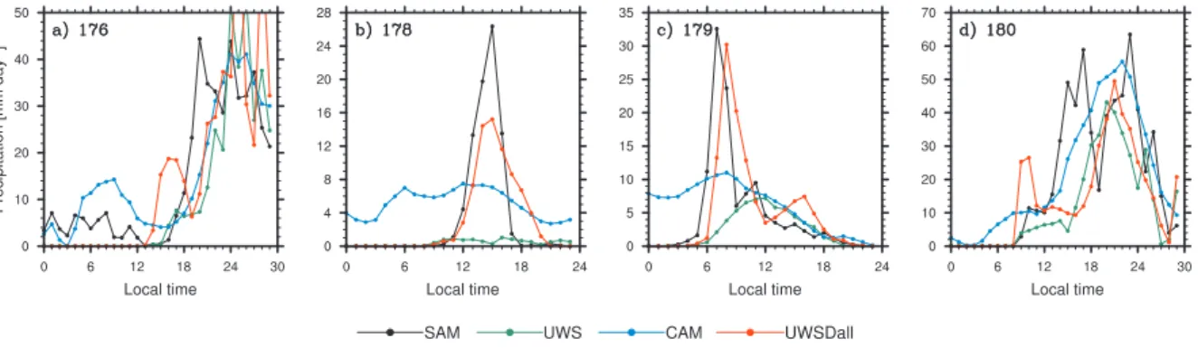
Figure 5 shows the diurnal cycle of precipitation for ARM days 176, 178, 179 and 180 for the simulations CAM, UWS, UWSDpbl and the SAM LES simulation. Day 174 exhibits similar features but is not included here for brevity. The de-fault CAM configuration shows too weak a diurnal rainfall modulation that causes excessive morning precipitation. This problem is especially visible on day 178, which constitutes the most archetypical example of surface forced convection during the period.
Both UWS and UWSDpbl better capture the timing of pre-cipitation. The onset of precipitation coincides with SAM on days 176, 178 and 180 (Fig. 5a, b, d), while it is de-layed on days 179 (Fig. 5c) and 174 (not shown). However, UWS and UWSDpbl also strongly underestimate the precip-itation amounts. The cloud-base improvements in UWSDpbl increase the simulated amounts on day 178 but the impact remains generally small. This is understandable; the cloud-base improvements only affect the simulation of strongly pre-cipitating convection; if the convection never produces sig-nificant rainfall, these improvements have no chance to mod-ify the simulation.
Fig. 5. Diurnal cycle of precipitation for ARM day(a)176,(b)178,(c)179, and(d)180. Black, green, blue and red lines are for SAM, UWS, CAM and UWSDpbl, respectively.
4 Entrainment
As in the previous section, we first employ the SAM sim-ulations to derive formsim-ulations for entrainment and detrain-ment that work for both shallow and deep convection. We then implement and test them in combination with our cloud-base property modifications with single-column model ex-periments.
4.1 SAM results
Our approach retains the idea of buoyancy sorting described in Sect. 2.2, in which entrainment and detrainment rates are computed asǫ=ǫ0χc2andδ=ǫ0(1−χc)2(i.e., Eqs. 5a and
b), but SAM is used to revise the formulation ofǫ0.
In order to estimateǫ0 from our SAM experiments, we
first computeǫandδusing the equations for a simple plume model, as given in Eqs. (1) and (2) and done in previous LES studies. We sample all the cloudy points to compute the updraft mass flux and average it over one-hour time in-tervals. For the updraft propertyψu, we choose the
mass-flux weighted frozen moist static energy since it is approxi-mately conserved (Sψ=0). The mass-flux weighted frozen
moist static energy is again sampled over all cloudy points and hourly averaged, while ψ corresponds to the domain and hourly averaged frozen moist static energy. Solving Eqs. (1) and (2) forǫ andδ, we can then computeǫofrom
the buoyancy sorting relations (5a)–(5b). This presupposes that entrainment and detrainment rates indeed follow buoy-ancy sorting principles.
The result of this procedure is shown in Fig. 6. Figure 6 shows as an illustration profiles ofǫoobtained for two
differ-ent times in the KWAJEX simulation. The black solid line is associated with shallow cumuli with cloud tops reaching up to 2 km. The red solid line is under deep convection. Fig-ure 6 serves to illustrate thatǫ0both varies with height and
with the convective phase. At any given height, the values are larger during shallow cumulus convection. This is
con-Fig. 6.Profiles ofǫ0for two illustrative examples during KWAJEX: black line for the shallow phase, red line for the deep convection phase. The solid lines are from the SAM output, while the dashed lines are obtained using Eqs. (9) and (10).
sistent with previous LES studies (e.g Kuang and Bretherton, 2006; Khairoutdinov and Randall, 2006). Such studies have hypothesized that deep convective clouds, because of their larger size, entrain less than shallow cumuli.
Based on Fig. 6, the following generalized profile is used to diagnoseǫ0:
ǫ0(z)=ǫ0(zcb)( z zcb
)α (9)
withzcb the height of the cloud base. αis implicitly
com-puted by specifyingǫ0 at two “anchor” heights within the
cumulus layer, namely the cloud base zcb and a reference
heightz1that roughly corresponds to the minimum height of
0.6 1 2 10−5
10−4 10−3 10−2
w
cb [m s
−1]
εo
(zcb
) [Pa
−1
]
100 101 102
10−5 10−4 10−3 10−2
RRcb [mm day−1]
εo
(z1
) [Pa
−1
]
KWAJEX ARM
a) b)
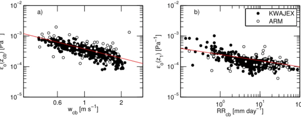
Fig. 7.Log-log scatter plots with regression line of(a)ǫ0(zcb)versuswcband(b)ǫ0(z1)versusRRcb. Full circles for KWAJEX, open circles for ARM. Regression lines in(a)and(b)are given by Eqs. (10b) and (10c), respectively. Panel(a)uses the full hourly statistics output from KWAJEX and ARM whereRRcb>0.1 mm day−1and 0< ǫ0(zcb) <0.002 Pa−1. This corresponds to 1076 and 61 points in KWAJEX and ARM, respectively. Panel(b)only considers the onset and mature phase whereRRcb>0.1 mm day−1and 0< ǫ0(z1) <0.002 Pa−1. This yields 482 and 59 points in KWAJEX and ARM, respectively.
The resulting relations read:
z1=zcb+2000 m (10a)
ǫ0(zcb)=4.1×10⁻³/(ρcbgwcb) (10b) ǫ0(z1)=exp(−8.3)×(max(RRcb,0.1))−0.2 (10c)
In these formulae,ǫ0is in Pa−1,RRcbin mm day−1,wcbis
the updraft velocity at cloud base (m s−1),ρ
cbis air density
at cloud base (kg m−3) andgis gravity. The velocity at cloud
base is computed from the SAM mass-flux weighted veloc-ity, sampled at all cloudy points and hourly averaged. Our specific choice ofz1is somewhat arbitrary; other choices can
produce similar results as long as Eq. (10c) is appropriately adapted.
Figure 7 shows scatter plots supporting Eqs. (10b)–(10c). Beginning from Fig. 7b and corresponding Eq. (10c),ǫ0(z1)
is set proportional to the inverse of the precipitation at cloud base. The correlation coefficient amounts to 0.6. An upper bound, obtained in Eq. (10c) by settingRRcb=
0.1 mm day−1, is set onǫ
0(z1)to avoid large values for small
precipitation amounts.
Covariability betweenǫ0 and precipitation, as displayed
by Fig. 7, is expected because higher precipitation amounts foster cold pool development which organizes the boundary layer. This produces larger and more coherent updrafts which have a lower bulk-mean entrainment rate, as noted above. Lower entrainment rates in turn favor the development of deeper clouds, hence sustaining a strong positive feedback betweenǫ0andRRcb.
Note that Fig. 7b only includes the onset/mature precipi-tation phase, as marked in Fig. 1, to determineǫ0(z1).
Dur-ing the decay phase, precipitation amounts are small, like in the onset phase, but mixing rates are small. Including those points in the regression reduces the slope of the regression line and results in too small mixing rates during the onset phase. This manifests itself by an overly rapid transition
to deep convection in the single-column model experiments. The overestimation implied by Eq. (10c) for the decay phase does not seem to have any detrimental effect on the simula-tions.
At cloud baseǫ0 is chosen inversely proportional to the
velocity at cloud base, as indicated in Fig. 7a and corre-sponding Eq. (10b). The correlation coefficient is 0.8. We do not useRRcb as a supplementary predictor since it does
not add significant skill to this regression. Usingwcbis
anal-ogous to the approach of Neggers et al. (2002), who proposed
ǫ=1/(wuτc), wherewu is the updraft velocity (m s−1) and τc=300 s is an empirical mixing timescale. In fact, our
for-mulation would implyǫ=4.1×10⁻³χ2
c/wcb, which yields
the same result for a typical cloud-base valueχc=0.9.
We also note that for values wcb= 0.5 m s−1 and zcb= 500 m typical of BOMEX, our formulation impliesǫ0=
8×10⁻³m−1=4/z
cb, which is at the low end of the range
of possible cloud-base values given in Table 1 of Park and Bretherton (2009) for the default UW scheme.
As a final illustration, the profiles ofǫ0reconstructed by
using Eqs. (9) and (10) and the SAM values forρcb,wcband RRcb, have been plotted as dotted lines in Fig. (6). Although
not perfect, the fit captures the overall shape of the bulk en-trainment rate profile and the corresponding difference be-tween the shallow and the deep phase.
The formulation ofǫ0in Eqs. (9)–(10) is admittedly
Fig. 8.Same as Fig. 5 but for SAM, UWS, CAM and UWSDall.
of precipitation at cloud base generalizes the specification of an inverse cloud radius as a predictor for entrainment rates (as in e.g. Kain, 2004) by allowing this radius to vary based on precipitation. Our approach can also produce similar re-sults to decreasing entrainment rate at high ambient relative humidity, a method successfully applied by Bechtold et al. (2008), to the extent that higher environmental relative hu-midity will correlate with deeper clouds that yield more pre-cipitation. Due to the strong feedback existing between en-trainment and precipitation, there is obviously a causality is-sue. Given that removing rain evaporation has been shown to yield smaller clouds, larger entrainment rates and less pre-cipitation (e.g. Khairoutdinov and Randall, 2006), there is some justification for usingRRcbas a predictor. This is also
consistent with principles of organization (Mapes and Neale, 2011).
The main difference to entrainment/detrainment formula-tions currently applied in convective parameterizaformula-tions is that Eqs. (9)–(10) do not require an explicit distinction between shallow and deep convection. Current formulations multiply their mixing rates by different prefactors. Here, through the production of precipitation and through changes in the envi-ronmental properties (as expressed byχc), the mixing rates
are allowed to vary with time and can support both shallow and deep convection. Equations (9)–(10) embody buoyancy sorting and organizational principles, which should apply to convection in general independently of the cloud depth. To which extent such a unified formulation can actually repro-duce convection is investigated in the next section.
4.2 SCAM experiments
The revised entrainment-detrainment formulation is tested in SCAM by introducing it into UWSDpbl. As in UWSDpbl, we employ the precipitation averaged over the last hour as a predictor forRRcb. wcbis diagnosed with Eq. (8b), while
the other terms in Eqs. (9)–(10) are directly available. Two other changes are made to the default mixing scheme. First, no water is detrained before performing buoyancy sorting, as
this tends to improve the results. Second,χc is limited to a
maximum value of 0.5 above 6 km to avoid the development of instabilities due to compensating subsidence in cases of an increasing mass flux with height. The new simulation is called UWSDall (see Table 1).
Figure 8 shows the diurnal cycle of precipitation for ARM days 176, 178, 179 and 180 for UWSDall, CAM, UWS and SAM. Comparison to Fig. 5 reveals a strong impact of the new entrainment formulation. UWSDall produces stronger precipitation than UWSDpbl. The amounts are of compara-ble magnitude to the SAM simulation. Despite a tendency to produce too large precipitation amounts at the beginning of the onset phase, UWSDall clearly improves the simulated precipitation diurnal cycle as compared to CAM. This is es-pecially true on day 178 (see Fig. 8b), where most convective parameterizations would fail (see Guichard et al., 2004).
UWSDall, in contrast to UWSDpbl, can realistically tran-sition to deep convection. In principle, the moistening of the environment during the day through detrainment from pre-vious shallow convection should increase χc, so the mass
flux decreases less rapidly with height and at some point sig-nificant mass flux reaches into the mid-troposphere. Nev-ertheless this effect did not appear sufficient in our single-column model experiments, in contrast to results from cloud-resolving studies (see especially Chaboureau et al., 2004). An additional and explicit sensitivity of fractional entrain-ment and detrainentrain-ment rates to precipitation is required for the UW scheme to realistically transition from shallow to deep convection with the right diurnal timing.
Fig. 9.Mean profiles of(a)cloud cover,(b)mass flux (kg m−2s−1),(c)relative humidity (%), and(d)temperature difference with respect to SAM (K) for ARM day 178. Lines as in Fig. 8. The profiles are averaged over the rain period, i.e., 10:00–18:00 LT. Panel(e)shows specific humidity (g kg−1) at 15:00 LT on ARM day 178.
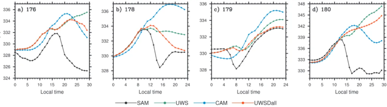
Fig. 10.Same as Fig. 8 but for MSE averaged over the lowest 1 km.
a function of relative humidity, the observed underestimation is sensitive to the chosen relative humidity threshold for the onset of cloud formation. The mass flux profile in UWS-Dall is much more similar to SAM, with only a slight re-maining underestimate of mass flux between 1.5 and 10 km. This good agreement implies that the new entrainment for-mulation is able to capture typical entrainment and detrain-ment rate profiles in ARM. Similar conclusions hold for other times and ARM days.
In terms of relative humidity and temperature, Fig. 9c, d indicates that UWSDall outperforms CAM and UWS. The UWSDall curve tends to agree well with the SAM re-sults. The relative performance of the simulations is case-dependent. Significant improvements are obtained on days 178 and 179 (in which the diurnal cycle of surface fluxes is the main convective forcing) while all simulations perform similarly on the remaining days, on which large-scale advec-tive forcing is more important (not shown).
One of the main biases of the simulations is visible in Fig. 9d and especially in Fig. 9e. Figure 9e shows specific humidity profiles at 15:00 LT, the time of maximum precipi-tation. CAM, UWSDall and UWS are all moister than SAM. They all exhibit a well-mixed boundary layer (see profile be-low about 1 km), while SAM only remains well mixed in the upper part of the PBL (between about 300–900 m).
respond to such changes.
Finally, Fig. 10 shows time series of MSE averaged over the lowest 1 km of the atmosphere, as a rough estimate for the PBL, for ARM. Figure 10 illustrates the other main de-ficiency of the single-column model experiments. All the SCAM simulations exhibit warmer MSE than SAM during the phase of heavy precipitation (compare to the precipita-tion time series in Fig. 8). The apparent missing stabilizaprecipita-tion of PBL MSE in SCAM is a direct consequence of not hav-ing explicit downdrafts in UWS and UWSDall. CAM does include downdrafts, but only saturated downdrafts. Yet most of the downdrafts appear to be unsaturated in SAM.
The absence of downdrafts in UWSDall does not preclude the use of Eqs. (6), (7), (9) and (10). Our approach recog-nizes that cold pools, whether created by subcloud evapora-tion as we can do in CAM, or created also by organized con-vective downdrafts as visible in SAM, affect the concon-vective development. The fact that UWSDall can track precipitation and exhibits some reduction in MSE in Fig. 10 indicates that our modifications can indeed introduce a feedback between convective rainfall and changes in the boundary layer struc-ture. The reported biases in MSE, especially towards the end of the different days, have no strong influence since we use prescribed large-scale forcing and simulate each day sepa-rately.
Figure 11 displays the results obtained for KWAJEX for the different simulations. We do not show precipitation since all the simulations perform well due to the use of a prescribed omega field. The different profiles in Fig. 11a–d have been averaged over the full time period. As in ARM we can rec-ognize the improvements in the simulated cloud cover and mass flux profiles in UWSDall as compared to CAM and UWS. UWSDall also captures the relative humidity profile very well, while both CAM and UWS tend to overmoisten the troposphere, especially above 3 and 1 km, respectively. Finally, no strong biases can be detected in the simulated temperature profile in UWSDall.
As in ARM, Fig. 11e reveals the bias toward a well-mixed PBL in the SCAM simulations. CAM and UWSDall ap-pear too cold and too dry, while they were too warm and too moist in ARM (Fig. 9d, e). Time series of mean PBL MSE (not shown) reveals that the depletion of MSE in CAM and UWSDall during the precipitating phase is similar both in ARM and KWAJEX. Since the depletion is much stronger in SAM in ARM than in KWAJEX due to stronger down-drafts, this results in a warm and moist (cold and dry) bias in ARM (KWAJEX). We thus conclude that the ventilation of the PBL is too strong in UWSDall, which partly compen-sates for the missing downdrafts. In opposition, UWS never exhibits a strong depletion in MSE and thus is characterized by a warm and moist bias in all the cases.
Finally, the results for BOMEX are displayed in Fig. 12 with profiles of liquid water potential temperature, total spe-cific humidity, cloud cover and mass flux for UWS, CAM, UWSDall and SAM. The profiles have been averaged over
hours 3 to 6 of the BOMEX integrations, as in Park and Bretherton (2009). CAM exhibits similar biases to those noted in Park and Bretherton (2009) with excessive cloud cover throughout the cumulus layer. This bias is mainly removed in UWS and UWSDall. Although differences ex-ist in the simulated profiles between UWS and UWSDall in Fig. 12, UWSDall is still able to simulate a typical case of shallow convection as well as UWS. In particular, with UWSDall, as with UWS, the simulated clouds remain shal-low. Employing the Zhang and McFarlane (1995) scheme as the sole convective parameterization in CAM would erro-neously simulate some deep convection for BOMEX.
Hence in terms of large-scale variables UWSDall agrees well with SAM in many respects. It provides improved single-column simulations of tropical oceanic, mid-latitude continental and shallow convection than the default version of the CAM model. It also gives more realistic simulations than UWS of both deep convection cases.
4.3 Sensitivity
In the previous section, we demonstrated that UWSDall com-pares better to SAM than either CAM or UWS. However, it remains to be shown whether all the included modifications are important for these improvements. From the results in Sect. 3 it is clear that the mixing rates need to be reformu-lated. The necessity of the changes in cloud-base mass flux and cloud-base thermodynamic properties are investigated in this section.
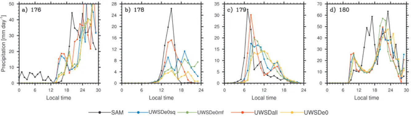
To that aim we perform three sensitivity experiments called UWSDe0, UWSDe0mf, and UWSDe0sq (see Ta-ble 1). UWSDe0 is identical to UWSDall except that it only includes entrainment/detrainment effects, not the modifications to TKE (Eq. 6) and thermodynamic proper-ties (Eqs. 7a, b). UWSDe0mf and UWSDe0sq build on UWSDe0: UWSDe0mf adds only the changes in cloud-base mass flux via changes in TKE (Eq. 6), while UWSDe0sq adds only the changes in cloud-base thermodynamic prop-erties (Eqs. 7a, b) via changes inσq.
Fig. 11.Same as Fig. 9 but for KWAJEX. The profiles in(a)–(d)have been averaged over the full time period, while panel(e)displays a specific time under strong precipitation (hour 230 in the simulation).
Fig. 12. Profiles of (a)liquid water potential temperature (K),(b) total specific humidity (g kg−1),(c)cloud cover and (d)mass flux (kg m−2s−1) averaged over hours 3 to 6 of BOMEX, for the same simulations as in the previous figures.
The increase in precipitation in UWSDe0mf and UWSDe0sq versus UWSDe0 follows from an increased mass flux at all heights. This stands in better agreement to the SAM values (not shown). The enhanced mass flux in UWSDe0mf is a direct consequence of both enhanced cloud-base mass flux and more frequent triggering of con-vection, as expected from Eq. (6). The enhanced mass flux in UWSDe0sq follows from an enhanced entrainment rate and decreased detrainment rate at cloud base, which thus al-low more plumes to be retained in the updraft. The latter changes inǫandδrelate to a value ofχclarger in UWSDe0sq
than in UWSDe0, as expected from the use of moister updraft parcels.
For most other variables, the differences between UWSDe0mf, UWSDe0sq and UWSDe0 are small, both in ARM and KWAJEX. The exceptions are of course the TKE values and the cloud-base thermodynamic properties.
Figure 14 displays scatter plots of TKE in SCAM versus SAM for the ARM, KWAJEX and BOMEX cases. On the left, we show UWS as an example for the simulations which do not include the TKE increase due to cold pool activity (i.e., UWS, UWSDe0, UWSDe0sq). On the right, UWSDall is chosen as an example for the two remaining simulations, where Eq. (6) is used.
As indicated by Fig. 14 and as expected, TKE is strongly underestimated in UWS (or equivalently UWSDe0 and
UWSDe0sq), while UWSDall (and UWSDe0mf) are in bet-ter agreement with SAM. The latbet-ter two simulations are able to capture the increase in TKE during precipitation events and thus confirm the appropriateness of Eq. (6). The overall underestimation in Fig. 14b is due to a slight underestima-tion of the boundary layer height in UWSDall. The points where a strong discrepancy between SCAM and SAM val-ues remains visible in Fig. 14b correspond to those times where UWSDall produces no or only weak precipitation, while SAM records strong precipitation.
In terms of cloud-base thermodynamic properties, the use of Eq. (7b) yields an increase in cloud-base MSE. This in-crease amounts to up to 2 K in UWSDe0sq (and UWSDall) with respect to UWSDe0 (or UWS, UWSDe0mf). Given the existing biases in the PBL (see Sect. 4.2) this agrees better with SAM for KWAJEX, but less well for ARM.
5 Conclusions
Fig. 13.Diurnal cycle of precipitation for ARM day(a)176,(b)178,(c)179, and(d)180. Black, blue, green, red and orange lines are for SAM, UWSDe0sq, UWSDe0mf, UWSDall and UWSDe0, respectively.
Fig. 14.Scatter plots of PBL averaged TKE in(a)UWS and(b)UWSDall versus SAM values. Black, white and red circles are for KWAJEX, ARM, and BOMEX, respectively. For KWAJEX and ARM, only points with precipitation are plotted. The BOMEX point corresponds to the mean over the simulation hours 3 to 6. A 1:1 line has also been added to the plots.
convection is precipitation, so that improving the representa-tion of some key effects of precipitarepresenta-tion in a shallow convec-tion scheme can allow it to be extended into a unified scheme. We considered previously studied cases of shallow con-vection (BOMEX), tropical oceanic concon-vection (KWAJEX) and mid-latitude continental convection (ARM). We used large-eddy simulations of the three cases as benchmarks for parameterization formulation and improvement. We imple-mented our improved relations in the UW shallow convection scheme and tested the results in the SCAM single-column modeling framework.
We included three main effects of precipitation on con-vective development, encompassing cloud-base mass flux, cloud-base humidity and entrainment/detrainment rates. Rain evaporation generates cold pools in the PBL, forcing convergence and thus favoring cloud formation. This ex-presses itself by an increase in boundary-layer TKE, which
in the UW scheme is a primary control on cloud-base mass flux. We found that the increase of TKE compared to that in the dry convective boundary layer scales with precipita-tion at cloud base times the height of the PBL (see Eq. 6). Rain evaporation also modifies the probability distribution function of cloud-base thermodynamic properties, increas-ing horizontal humidity variance. Cumulus updrafts tend to form over the moister parts of the PBL, so to predict cumu-lus base humidity we explicitly include a parameterization of humidity variance in terms of cloud-base precipitation rate (see Eq. 7). Finally, the formation of cold pools organizes the planetary boundary layer and the entire cumulus ensem-ble and indirectly lowers the bulk entrainment rateǫ0. This
These modifications were implemented in the UW shallow convection scheme. In all cases, the new scheme performs as well as or better than the default CAM version. It also out-performs the simulations using the default UW shallow con-vection scheme as the sole convective parameterization. For our tropical oceanic convection case, the new unified scheme especially improves relative humidity, cloud cover and mass flux profiles. The performance in terms of mid-latitude con-tinental convection is more case-dependent. The main im-provement is in the simulated timing of the diurnal cycle when surface fluxes are the dominant forcing for convection. The new unified scheme removes the premature onset of pre-cipitation, which is a common pitfall of deep convective pa-rameterizations, and is able to simulate the peak rainfall rate and duration of rainfall reasonably well. Finally, the scheme can still realistically simulate shallow oceanic trade-cumulus convection.
The main biases, which are present not only with the new scheme but in all of our single-column model experiments, are that the simulated PBL structure tends both to be too well mixed and to insufficiently reduce boundary-layer MSE dur-ing deep convection as compared to LES, especially for mid-latitude continental convection. We attribute those biases to a combination of two factors. First, to maintain convection, the PBL schemes must sustain a convective PBL that extends from the surface to the convective cloud base. Second, the UW convection scheme does not explicitly consider down-drafts, while the Zhang and McFarlane (1995) scheme only includes saturated downdrafts. Yet most of the downdrafts appear to be unsaturated in the LES.
Of the three tested modifications (i.e., in cloud-base mass flux, cloud-base thermodynamic properties and bulk entrain-ment rate), changing the bulk updraft lateral mixing rate has the largest impact. Without this, the UW scheme has difficulty in simulating a realistic transition from shallow to deep convection. This is true even though its buoyancy sorting algorithm should allow it to be sensitive to free-tropospheric relative humidity and previous cloud-resolving modeling studies (e.g., Chaboureau et al., 2004) have indi-cated that moistening of the troposphere through detrainment from shallow and/or congestus clouds controls the transition to deep convection. Expressed in other words, precipitation (or its evaporation) is a strong positive feedback in the tran-sition from shallow to deep convection in our single-column model experiments, which helps explain why this transition is rather difficult for cumulus parameterizations to simulate. The impacts of our modifications made to the cloud-base mass flux and cloud-base thermodynamic properties are sub-tler. Separately, they only have small impacts but taken to-gether, they enhance the sensitivity of convection to prior precipitation and enhance the precipitation peaks. Their in-clusion seems especially important for the timing and ampli-tude of the convective diurnal cycle over mid-latiampli-tude conti-nental areas.
All in all our approach does allow for a unified represen-tation of moist convection. It also allows for a representa-tion of the organizarepresenta-tional effects of precipitarepresenta-tion, which have been shown of importance for convection and are generally not included in convective parameterizations. Finally, it al-lows for tighter interactions between the planetary boundary layer and convection. Although included in the convection scheme, our modifications directly affect the mean bound-ary layer properties through the tight coupling produced by the use of a CIN/TKE closure. As indicated in Fletcher and Bretherton (2010), this type of closure maintains the cumu-lus base near the top of the PBL: an increase in cloud-base mass flux due to cold pool effects will feed back on the height of the PBL, thereby affecting the PBL properties. This is an advance over existing PBL schemes. Our proposed modi-fications are consistent even without explicitly including a downdraft scheme. Our approach recognizes that cold pools, whether created by subcloud evaporation, or created also by organized convective downdrafts, affect the convective de-velopment. Cold pools only require spatially localized rain evaporation in the PBL, not coherent downdrafts descending from high above the PBL top; in fact the downdrafts in trop-ical marine convection are not very organized or deep.
Our approach may be criticized as quite empirical and bi-ased towards the employed sampled data. As KWAJEX con-tains many data points and exhibits weak variability, it has the strongest influence on the estimated coefficients. Nev-ertheless we still considered quite a large data sample and built our different relations on theoretical expectations. The simplicity of the derived relations allows for an easy im-plementation/testing with other mass flux schemes, as long as such schemes employ a closure related to the PBL state. It also serves as a good proof of concept for our working hypothesis, letting room for more elaborate future refine-ments. Key unresolved issues remain the formulation of un-saturated downdrafts and a better theoretical foundation for formulating appropriate entrainment/detrainment rates, both issues with which deep convective parameterizations have been struggling for a long time. As a next step, global cli-mate model simulations with CAM will be performed with the new unified scheme.
Acknowledgements. The authors would like to thank Peter Blossey for the SAM simulations. The first author was funded by the Swiss National Science Foundation under the fellowship program for ad-vanced researchers, project PA00P2 124153. Chris Bretherton was funded by NSF grant ATM 0425247 to the CMMAP Science and Technology Center. Comments by the editor and the anonymous reviewers, which help simplifying our relations and improved our manuscript, are gratefully acknowledged.
References
Arakawa, A.: The cumulus parameterization problem: Past, present, and future, J. Climate, 17, 2493–2525, 2004.
Arakawa, A. and Schubert, W. H.: Interaction of a cumulus cloud ensemble with large-scale environment, Part 1, J. Atmos. Sci., 31, 674–701, 1974.
Bechtold, P., Chaboureau, J. P., Beljaars, A., Betts, A. K., Kohler, M., Miller, M., and Redelsperger, J. L.: The simulation of the diurnal cycle of convective precipitation over land in a global model, Q. J. Roy. Meteorol. Soc., 130, 3119–3137, 2004. Bechtold, P., Kohler, M., Jung, T., Doblas-Reyes, F., Leutbecher,
M., Rodwell, J., Vitart, F., and Balsamo, G.: Advances in sim-ulating atmospheric variability with the ECMWF model: From synoptic to decadal time-scales, Q. J. Roy. Meteorol. Soc., 134, 1337–1351, 2008.
Blossey, P. N., Bretherton, C. S., and Cetrone, J.: Cloud-resolving model simulations of KWAJEX: Model sensitivities and com-parisons with satellite and radar observations, J. Atmos. Sci., 64, 1488–1508, 2007.
Bretherton, C. S.: Challenges in Numerical Modeling of Tropi-cal Circulations. In The Global Circulation of the Atmosphere, edited by: Schneider, T. and Sobel, A. H., Princeton University Press, USA, 302–330, 2007.
Bretherton, C. S. and Park, S.: A new moist turbulence parame-terization in the Community Atmosphere Model, J. Climate, 22, 3422–3448, 2009.
Bretherton, C. S., McCaa, J. R., and Grenier, H.: A new parameteri-zation for shallow cumulus convection and its application to ma-rine subtropical cloud-topped boundary layers. Part I: Descrip-tion and 1D results, Mon. Weather Rev., 132, 864–882, 2004. Chaboureau, J. P., Guichard, F., Redelsperger, J. L., and Lafore,
J. P.: The role of stability and moisture in the diurnal cycle of convection over land, Q. J. Roy. Meteorol. Soc., 130, 3105–3117, 2004.
Chikira, M. and Sugizama, M.: A cumulus parameterization with state-dependent entrainment rate, Part I: Description and sensi-tivity to temperature and humidity profiles, J. Atmos. Sci., 67, 2171–2193, 2010.
Collins, W. D., Rasch, P. J., Boville, B. A., Hack, J. J., McCaa, J. R., Williamson, D. L., Briegleb, B. P., Bitz, C. M., Lin, S. J., and Zhang M.: The formulation and atmospheric simulation of the Community Atmosphere Model Version 3 (CAM3), J. Climate, 19, 2144–2161, 2006.
Dai, A. G., Giorgi, F., and Trenberth, K. E.: Observed and model-simulated diurnal cycles of precipitation over the contiguous United States, J. Geophys. Res., 104, 6377–6402, 1999. Deardorff, J. W.: Usefulness of liquid-water potential temperature
in a shallow-cloud model, J. Appl. Meteor., 15, 98–102, 1976. Deng, L. P. and Wu, X. Q.: Effects of convective processes on
GCM simulations of the Madden-Julian Oscillation, J. Climate, 23, 352–377, 2010.
Emanuel, K. A.: A scheme for representing cumulus convection in large-scale models, J. Atmos. Sci., 48, 2313–2335, 1991. Fletcher, J. K. and Bretherton, C. S.: Evaluating boundary
layer-based mass flux closures using cloud-resolving model simula-tions of deep convection, J. Atmos. Sci., 67, 2212–2225, 2010. Grandpeix, J. Y., Lafore, J. P., and Cheruy, F.: A density current
pa-rameterization coupled with Emanuel’s convection scheme, Part II: 1D simulations, J. Atmos. Sci., 67, 898–922, 2010.
Guichard, F, Petch, J. C., Redelsperger, J. L., Bechtold, P., Chaboureau, J. P., Cheinet, S., Grabowski, W., Grenier, H., Jones, C. G., Kohler, M., Piriou, J. M., Tailleux, R., and Tomasini, M.: Modelling the diurnal cycle of deep precipitating convection over land with cloud-resolving models and single-column models, Q. J. Roy. Meteorol. Soc., 130, 3139–3172, 2004.
Hack, J. J.: Parameterization of moist convection in the National Center for Atmospheric Research Community Climate Model (CCM2), J. Geophys. Res., 99, 5551–5568, 1994.
Hack, J. J. and Pedretti, J. A.: Assessment of solution uncertainties in single-column modeling frameworks, J. Climate, 13, 352–365, 2000.
Holtslag, A. A. M. and Boville, B. A.: Local versus nonlocal bound-ary layer diffusion in a global climate model, J. Climate, 6, 1825– 1842, 1993.
Kain, J. S.: The Kain-Fritsch convective parameterization: an up-date, J. Clim. Appl. Meteorol., 43, 170–181, 2004.
Khairoutdinov, M. F. and Randall, D. A.: Cloud Resolving Mod-eling of the ARM Summer 1997 IOP: Model Formulation, Re-sults, Uncertainties, and Sensitivities, J. Atmos. Sci., 60, 607– 625, 2003.
Khairoutdinov, M. F. and Randall, D. A.: High-resolution simula-tion of shallow-to-deep convecsimula-tion transisimula-tion over land, J. Atmos. Sci., 63, 3421–3436, 2006.
Kuang, Z. and Bretherton, C. S.: A mass-flux scheme view of a high-resolution simulation of a transition from shallow to deep cumulus convection, J. Atmos. Sci., 63, 1895–1909, 2006. Lee, M. I., Schubert, S. D., Suarez, M. J., Held, I. M., Lau, N. C.,
Ploshay, J. J., Kumar, A., Kim, H. K., and Schemm, J. K. E: An analysis of the warm-season diurnal cycle over the continental United States and northern Mexico in general circulation models, J. Hydrometeorol., 8, 344–366, 2007.
Li, L. J., Wang., B., Wang, Y. Q., and Wan, H.: Improvements in cli-mate simulation with modifications to the Tiedtke convective pa-rameterization in the grid-point atmospheric model of IAP LASG (GAMIL), Adv. Atmos. Sci., 24, 323–335, 2007.
Lin, J. L.: The double-ITCZ problem in IPCC AR4 coupled GCMs: Ocean-atmosphere feedback analysis, J. Climate, 20, 4497– 4525, 2007.
Mapes, B.E and Neale, R. B.: Parameterizing convective organiza-tion, J. Adv. Model. Earth Syst., 3, M06004, 2011.
Neale, R., Richter, J. R., and Jochum, M.: The impact of convec-tion on ENSO: From a delayed oscillator to a series of events, J. Climate, 21, 5904–5924, 2008.
Neggers, R. A. J., Siebesma, A. P., and Jonker H. J. J.: A multiparcel model for shallow cumulus convection, J. Atmos. Sci., 1655– 1668, 2002.
Park, S. and Bretherton, C. S.: The University of Washington shal-low convection and moist turbulence schemes and their impact on climate simulations with the Community Atmosphere Model, J. Climate, 22, 3449–3469, 2009.
Plant, R. S.: A review of the theoretical basis for bulk mass flux con-vective parameterization, Atmos. Chem. Phys., 10, 3529–3544, doi:10.5194/acp-10-3529-2010, 2010.
Randall, D. A., Khairoutdinov, M., Arakawa, A., and Grabowski, W.: Breaking the cloud parameterization deadlock, B. Am. Me-teorol. Soc., 84, 1547–1564, 2003.
transport on the atmospheric circulation in the Community At-mospheric Model, version 3 (CAM3), J. Climate, 21, 1487– 1499, 2008.
Rio, C., Hourdin, F., Grandpeix, J. Y., and Lafore, J. P.: Shifting the diurnal cycle of parameterized deep convection over land, Geophys. Res. Lett., 36, L07809, doi:10.1029/2008GL036779, 2009.
Siebesma, A. P., Bretherton, C. S., Brown, A., Chlond, A., Cuxart, J., Duynkerke, P. G., Jiang, H., Khairoutdinov, M., Lewellen, D., Moeng, C. H., Sanchez, E., Stevens, B., and Stevens, D. E. : A large-eddy simulation intercomparison study of shallow cumulus convection, J. Atmos. Sci., 60, 1201–1219, 2003.
Slingo, J. M., Sperber, K. R., Boyle, J. S., Ceron, J. P., Dix, M., Dugas, B., Ebisuzaki, W., Fyfe, J., Gregory, D., Gueremy, J. F., Hack, J., Harzallah, A., Inness, P., Kitoh, A., Lau, W. K. M., McAvaney, B., Madden, R.,Matthews, A., Palmer, T. N., Park, C. K., Randall, R., and Renno, N.: Intraseasonal oscillations in 15 atmospheric general circulation models: Results from an AMIP diagnostic subproject, Clim. Dynam., 12, 325–257, 1996.
Wang, Y. Q., Zhou, L., and Hamilton, K.: Effect of convective en-trainment/detrainment on the simulation of the tropical precipi-tation diurnal cycle, Mon. Weather Rev., 135, 567–585, 2007. Yang, G. Y. and Slingo, J.: The diurnal cycle in the Tropics, Mon.
Weather Rev., 129, 784–801, 2001.
Zhang, B. J. and McFarlane, N. A.: Sensitivity of climate simula-tions to the parameterization of cumulus convection in the Cana-dian Climate Centre general circulation model, Atmos.-Ocean, 33, 407–446, 1995.