Annales
Geophysicae
Predictions of the arrival time of Coronal Mass Ejections at 1 AU:
an analysis of the causes of errors
M. Owens and P. Cargill
Space and Atmospheric Physics, The Blackett Laboratory, Imperial College, London SW7 2BW, UK Received: 21 March 2003 – Revised: 7 July 2003 – Accepted: 11 July 2003 – Published: 1 January 2004
Abstract. Three existing models of Interplanetary Coronal
Mass Ejection (ICME) transit between the Sun and the Earth are compared to coronagraph and in situ observations: all three models are found to perform with a similar level of accuracy (i.e. an average error between observed and pre-dicted 1 AU transit times of approximately 11 h). To improve long-term space weather prediction, factors influencing CME transit are investigated. Both the removal of the plane of sky projection (as suffered by coronagraph derived speeds of Earth directed CMEs) and the use of observed values of solar wind speed, fail to significantly improve transit time prediction. However, a correlation is found to exist between the late/early arrival of an ICME and the width of the preced-ing sheath region, suggestpreced-ing that the error is a geometrical effect that can only be removed by a more accurate determi-nation of a CME trajectory and expansion. The correlation between magnetic field intensity and speed of ejecta at 1 AU is also investigated. It is found to be weak in the body of the ICME, but strong in the sheath, if the upstream solar wind conditions are taken into account.
Key words. Solar physics, astronomy and astrophysics
(flares and mass ejections) – Interplanetary physics (inter-planetary magnetic fields; sources of the solar wind)
1 Introduction
Coronal mass ejections (CMEs) are known to be the ma-jor cause of severe geomagnetic disturbances, now often re-ferred to as space weather (e.g. Daglis, 2001; etc.). In view of the possible deleterious effect of space weather on space-and ground-based technical systems (e.g. spacecraft charg-ing, lowering of orbit, communication interruptions, flow of induced currents along transmission lines), making a predic-tion of the arrival time of a CME at 1 AU, and its properties at that time, is highly desirable. In principle, one would like
Correspondence to:M. Owens
to be able to continually monitor the Sun using both full-disk imagers and coronagraphs (e.g. St. Cyr et al., 2000), so that an Earth-bound CME can be readily identified, and its veloc-ity, trajectory and spatial extent estimated. At present such observations are carried out by instruments on the Solar and Heliospheric Observatory (SOHO) spacecraft, although esti-mating these parameters is fraught with difficulties.
Other information on the properties of CMEs comes from in situ magnetic field and plasma measurements in the inter-planetary medium (especially at 1 AU), where they are usu-ally referred to as Interplanetary CMEs (ICMEs). Combin-ing observations at 1 AU with those of the Sun then permits a direct association to be made in many cases between a solar event and its interplanetary manifestation (but as will be dis-cussed later, this becomes difficult at solar maximum when CMEs are very common). One can then build up a picture of how the arrival time and speed of an ICME at 1 AU is re-lated to the velocity at the Sun, with the ultimate aim of de-veloping a forecasting tool which uses solar observables to make predictions at 1 AU. This has been attempted by some workers (e.g. Gopalswamy et al., 2000, 2001a; Vrˇsnak and Gopalawamy, 2002), and the details of these models will be discussed further in Sect. 2.
Since it is now clear that the transit time of a CME from the Sun to 1 AU is in the region of 1–5 days, advance forecasting is, in principle, feasible. However, there are problems with such forecasting models due to (a) the difficulty in estimating the velocity and trajectory of the CME at the Sun with single spacecraft observations, (b) analysing ICMEs using single-point in situ measurements and (c) understanding the forces that act on the ICME in the interplanetary medium.
St. Cyr et al., 2000.) Tracking a CME feature (usually the bright leading edge) in consecutive coronagraph images al-lows for the speed of the CME to be estimated. However, this coronagraph-derived speed is the component of the CME speed in the plane of the sky (i.e. the plane perpendicular to the Sun-observer line). Thus, for any non-limb CME (such as a halo event), measurements of speed and direction will suffer to some degree from a “projection effect” (e.g. Gopal-swamy et al., 2000). So tracking a halo gives the expan-sion speed of a CME rather than its radial speed away from the Sun, and the precise trajectory and velocity of the CME hence cannot be determined with any guaranteed accuracy.
In the heliosphere, ICMEs can be identified in magnetic field and plasma data by an enhanced magnetic field magni-tude and sometimes a reduced proton temperature (both last-ing for of the order of 0.5–1 day at 1 AU). Furthermore, ap-proximately half the ICMEs show a smooth rotation in the magnetic field direction (referred to as “magnetic clouds”: Burlaga, 1988). ICMEs are clearly large three-dimensional structures that are undergoing continual expansion as they pass 1 AU. They are often preceded by a shock wave and compressed sheath region. On the basis of single spacecraft observations, further assumptions are needed to infer their 3-D structure, and in particular, which part of the ICME one is actually sampling.
ICME speeds at 1 AU range from 400 km/s up to in excess of 700 km/s, close to that of the ambient solar wind. This should be contrasted with estimated speeds at the Sun rang-ing from 100–2000 km/s. Clearly the interaction of ICMEs with the ambient solar wind leads to a net “equalisation” of the respective velocities (e.g. Gopalswamy et al., 2000), a process that can be attributed to a process analogous to aero-dynamic drag (Cargill et al., 1995; Vrˇsnak and Gopalswamy, 2002). However, difficulties in understanding this drag make prediction of the ICME speed at 1 AU difficult.
This paper will discuss the forecasting of ICME proper-ties at 1 AU, and in particular, focus on possible causes for the systematic error in arrival time of around 15% that these models give. Section 2 reviews the existing models. Sec-tion 3 summarises the data used in our analysis, and exam-ines model error and Sect. 4 addresses causes of the error (projection effects, ambient solar wind properties and ambi-guities of observations at 1 AU).
2 A summary of current ICME forecasting models
The present generation of forecasting models all predict the transit time of a CME to 1 AU. This time (τ) is defined as being the time between the first observation of the CME by a coronagraph, and the arrival of the leading edge of the ICME at 1 AU. For example, the leading edge of a magnetic cloud event is simply defined as the onset of the smooth field rotation and proton temperature reduction. For non-cloud events, the identification is somewhat more difficult, and varies slightly between different ejecta. Signatures used in-cluded the onset of a reduced proton temperature or density,
the start of a linearly declining velocity profile and a reduced variance in the magnetic field. The sole input for the models is the earthward speed of the CME in the corona (U). A brief outline of each model follows.
2.1 Gopalswamy et al. (2000) model: constant acceleration or deceleration
As we noted in the Introduction, CMEs exhibit a much wider range of speeds at the Sun (100–2000 km/s: Hundhausen, 1999; St. Cyr et al., 2000) than at 1 AU (300–1000 km/s; Gopalswamy et al., 2001a). If one notes that the velocity of the solar wind ahead of and behind an ICME is in the range 350–600 km/s, ICMEs are, depending on their speed relative to the solar wind, either accelerated or decelerated towards the solar wind speed. Gopalswamy et al. (2000) assumed that the acceleration was constant between the Sun and 1 AU, so that the total effective interplanetary acceleration (a1) under-gone by an ICME is:
a1=
V (1 AU)−U
τ , (1)
whereV (1 AU)is the ICME speed at 1 AU. Assuming such a constant acceleration, the travel time of the CME is then given by the solution of the simple kinematic relation: S=U τ+1
2a1τ 2,
(2) whereSis the distance travelled (1 AU). We refer to this as the G2000 model.
2.2 Gopalswamy et al. (2001a) model: cessation of accel-eration before 1 AU
Gopalswamy et al. (2001a) noted that the G2000 model could not account for the observation that CMEs with a slow initial speed (U < 500 km/s) have an approximately constant ar-rival time of 4.2 days. The G2000 model was thus modified by assuming that ICME acceleration ceased at a heliocentric distance of 0.76 AU for all CMEs, irrespective of their initial speed (0.76 AU was found to best fit the data). Thus, the total transit time to 1 AU is the sum of the travel time to 0.76 AU at constant acceleration, and the travel time from 0.76 AU to 1 AU at constant speed:
τ = −U+
p
U2+2a 2d a2
+p1 AU−d
U2+2a 2d
, (3)
where a2 is an effective interplanetary acceleration, that is now derived empirically from quadrature observations of CMEs (see Sect. 3.2), anddis the acceleration cessation dis-tance (0.76 AU in the present case). We refer to this as the G2001 model.
2.3 Vrˇsnak and Gopalswamy (2002) model: aerodynamic drag
beyond a fraction of an AU. Magnetic forces may act well beyond their usual pre-supposed location in the inner corona (e.g. Chen, 1996), and will be discussed later. However, the major cause of deceleration in the interplanetary medium is likely to be the interaction of the ICME with the ambient plasma. In reality, this will be a complex collection of pro-cesses involving shock waves, generation of turbulence, etc., but these are often parameterised as an aerodynamic drag force of the formACD(V −W )|V −W|, where V is the speed of the centre of mass of the ICME,Wis the solar wind speed,CD is a drag coefficient, typically a number of order unity (Chen, 1989, 1996; Cargill et al., 1995, 1996) andAis the cross section of the ICME.
Vrˇsnak and Gopalswamy (2002) proposed a model for es-timating the ICME transit time when the only force acting upon the ICME in interplanetary space is the aerodynamic drag. They assumed that the drag force was linearly pro-portional to the relative velocity. (They demonstrated that this leads to little difference from a model where the drag was proportional to the square of the relative velocity, and we have confirmed this independently for the cases shown in this paper.) The equation of motion of an ICME at some he-liocentric distanceR(R=r/rs, wherers is the solar radius) is then:
dV dτ =αR
−β(V−W ),
(4) whereαandβ are constants that parameterise the drag as a function of distance, and are determined from a best fit to the data (see below). The solar wind speed is given by Sheeley et al. (1997):
W (R)=Wo
r
1−e2.8−R
8.1 , (5)
whereW0is the asymptotic solar wind speed. Writing this in terms ofRgives:
dV
dR =rsαR −β
1−W
V
. (6)
Numerical integration from the low corona (R =10, where it is assumedV =U) to 1 AU then givesv(R), and henceτ. This is referred to as the VG2002 model.
3 Assessment of the three models
3.1 Solar and interplanetary data
We now compare these models with observations of CME transit times. The required observations are the CME speeds and onset times at the Sun obtained from coron-agraph observations, and the arrival times and speeds at 1 AU from in situ solar wind magnetic field and plasma measurements. Our main focus is on the interval starting in November 1997, when the Advanced Composition Ex-plorer (ACE) spacecraft made its first measurements of the solar wind, to April 2001. Coronal observations of CMEs
were made by the Large Angle Spectroscopic Coronagraph (LASCO: Brueckner et al., 1995) on the SOHO spacecraft. The onset time and speed of halo CMEs were taken from the LASCO CME catalogue (complied by S. Yashiro, G. Michalek and N. Gopalswamy: see http://cdaw.gsfc.nasa. gov/CME list/index.html). In situ plasma and magnetic field data from the SWEPAM (McComas et al., 1998) and MAG (Smith et al., 1998) instruments on board ACE were used to identify ICMEs at 1 AU.
We note here that the onset times from this catalogue should not be confused with the actual “onset” of the CME at the Sun. The “onset time” in the LASCO catalogue is de-fined as the time of CME appearance in the C2 coronagraph, which has an occulting disc of radius 2rs, so that the CME transit distance used in this study will be somewhat less than 1 AU. However, the error in the start time may be exagger-ated for cases when the CME is directed earthwards. For halo CMEs the precise altitude of the “onset” measurement depends upon their true angular extent: an angular width of 40◦(80◦) will result in an altitude of 3.7rs(1.2rs). Using the average speed of the CMEs in this study (669 km/s), results in an error in the onset time of∼40 min and as we shall see, this is small compared to the average transit time error.
Connecting observations of CMEs at the Sun and ICMEs at 1 AU is not trivial. When multiple halo CMEs are seen (as occurs frequently at times of solar maximum), simple argu-ments about the association of ICMEs with CMEs should be avoided as not all front-side halo CMEs lead to a recognis-able ICME signature at 1 AU. Furthermore, multiple CMEs originating from the same source region, or regions with a small angular separation (i.e. comparable to half the average CME width∼36◦), within a day of each other, could lead to significant interaction between different CMEs (Gopal-swamy et al., 2001b). In order to focus in particular on the interplanetary forces acting on ICMEs, this study is restricted to cases where there is no ambiguity between solar and inter-planetary observations. Hence, periods containing multiple halo CMEs were excluded.
Table 1.The five additional CME-ICME pairs.
ICME CME Transit time (days)
Date UT V (km/s) Date UT U(km/s)
28 Jan 1998 19:40 375 25 Jan 1988 15:22 693 4.18
12 Aug 2000 05:02 586 9 Aug 2000 16:34 702 2.52
13 Oct 2000 16:48 402 9 Oct 2000 23:46 798 3.71
29 Oct 2000 00:00 380 25 Oct 2000 08:24 770 3.65
28 Apr 2001 16:34 666 26 Apr 2001 12:29 1006 2.17
0 200 400 600 800 1000 1200 1400 1600 1800 −8
−7 −6 −5 −4 −3 −2 −1 0 1 2x 10
−3
Vcme (km/s)
IP Acc
n (km/s 2)
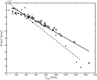
Fig. 1. The interplanetary acceleration as a function of the CME speed (U) at the Sun. The open circles correspond to the 35 CME – ICME pairs observed along the Earth-Sun line and the solid line shows the linear fit:a1(km/s2)= −10−3[0.0040U (km/s)−1.8].
The plus signs correspond to the 19 CME – ICME pairs observed in quadrature, and the dashed line shows the linear fit:a2(km/s2)= −10−3[0.0054U (km/s)−2.2].
Gopalswamy et al. (2001a) published a list of 47 CME-ICME pairs using data from the WIND spacecraft and LASCO, 12 of which occurred before ACE became operational. A further 5 event pairs were excluded from this study as being multiple halos. Five events that do not appear in their list were used in this study. Thus, 30 CME-ICME pairs are common to both studies. In the interest of brevity, events common to both surveys are not listed here. Events 1–12 and 16 of Gopalswamy et al. (2001a) were not used due to lack of ACE data, while events 25, 30, 32 and 41 were not included due to insufficient confidence in the association. Table 1 lists the additional events in a similar format to Gopalswamy et al. (2001a).
A second data set used in this study consists of quadrature observations of CMEs (i.e. remote coronagraph observations made from the Earth-Sun line, and quadrature in situ mea-surements of ICMEs made over the limb of the Sun). Lind-say et al. (1999) compiled a list of such events using the Solar
0 200 400 600 800 1000 1200 1400 1600 1800 1
1.5 2 2.5 3 3.5 4 4.5 5
CME speed (km/s)
Transit Time (days)
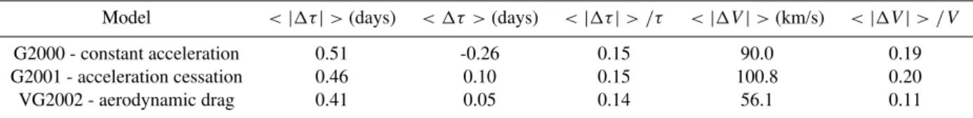
Fig. 2.The transit time of a CME to 1 AU as a function of the CME speed for the 35 E-S line events. The solid, dashed and dotted lines represent the transit time predicted by models G2000, G2001 and VG2002, respectively.
Maximum Mission (SMM) and Solwind coronagraphs, and the Helios 1 and Pioneer Venus Orbiter (PVO) in situ mag-netic field and plasma measurements. Our study uses the slightly modified list of 19 events published by Gopalswamy et al. (2001a). The in situ observations of these ICMEs were made at heliocentric distances ranging from 0.63 to 0.92 AU. 3.2 Errors in the models
The circles in Fig. 1 show the effective interplanetary accel-eration (a1) undergone by the 35 E-S line CMEs as a function of their coronal speed (U). From the G2000 model, a linear fit to the data (solid line) is given by:
a1(km/s2)= −10−3[0.0040U (km/s)−1.8], (7) and we note that Gopalswamy et al. (2000) found a similar result for their list of E-S line CMEs:
Table 2.Comparison of models with the observations of the 35 E-S line CMEs.
Model <|1τ|>(days) < 1τ >(days) <|1τ|> /τ <|1V|>(km/s) <|1V|> /V
G2000 - constant acceleration 0.51 -0.26 0.15 90.0 0.19
G2001 - acceleration cessation 0.46 0.10 0.15 100.8 0.20
VG2002 - aerodynamic drag 0.41 0.05 0.14 56.1 0.11
if constant acceleration is assumed. Figure 2 shows the ob-served transit time (circles) as a function of CME speed, with the solid line showing the transit time predicted by the G2000 model. The average error between the predicted and actual transit times(< |1τ| >)is 0.51 days and the fractional er-ror<|1τ| > /τ =0.15. The distribution of1τ is skewed (< 1τ >= −0.26), and hence, the G2000 model systemat-ically overestimates CME transit times. Figure 3 shows the ICME speed (averaged over the duration of the event) for ejecta along the E-S line (circles) and the quadrature events (crosses) as a function of the CME speed at the Sun. For the G2000 model, the average error(< 1V >)is 90.1 km/s and the percentage error(< 1V > /V )is 0.19. The quality of the fit of the G2000 and G2001 models are discussed more fully in Gopalswamy (2002).
The crosses in Fig. 1 indicate the interplanetary accelera-tion for the 19 quadrature observaaccelera-tions. The linear fit is given by:
a2(km/s2)= −10−3[0.0054U (km/s)−2.2] (9) (Gopalswamy et al., 2001) and is shown by the dashed line on Fig. 1. Assuming a constant acceleration of magnitude a2 to 0.76 AU, and then a constant ICME speed to 1 AU, the G2001 model B then gives < |1τ| >= 0.46 days, < 1τ >=0.10,<|1τ|> /τ =0.15,< 1V >=108 km/s and< 1V > /V =0.2 (dashed line on Figs. 2 and 3). Note that use of Eq. (9) in the G2000 model will lead to an increase in<|1τ|>due to longer travel times of faster CMEs.
Vrˇsnak and Gopalswamy (2002) used aerodynamic drag coefficients of α = −0.002 and β = 1.5, and a solar wind speed at 1 AU (Wo) of 400 km/s. In this study these three parameters were allowed to vary so as to minimise the difference between the predicted and actual 1 AU tran-sit times (1τ). A simplex search method was used (Lagarias et al., 1998). We find that α = −0.0021, β = 1.34 and Wo = 438.1 km/s gives the best fit. Using these parame-ters in the VG2002 model then gives<|1τ|>=0.41 days, < 1τ >=0.05,<|1τ|> /τ =0.14,< 1V >=56 km/s and< 1V > /V =0.11 (dotted line on Figs. 2 and 3).
The results for the three models are summarised in Table 2, which also shows the average and percentage errors in the ve-locity at 1 AU (1V: right-hand columns). It should be noted that despite the considerable difference in the assumptions in each of the models, the average error in the transit time is effectively the same for all three models. The VG2001 model appears to do somewhat better in the prediction of the ICME velocity at 1 AU. We also examined how the results
0 200 400 600 800 1000 1200 1400 1600 1800 300
400 500 600 700 800 900 1000
CME speed (km/s)
Average ICME speed (km/s)
Fig. 3. The CME speed as a function of the average ICME speed at 1 AU for the 35 events observed along the Earth-Sun line (“o”s) and the 19 events observed in quadrature (“+”s). The solid, dashed and dotted lines represent the ICME speeds at 1 AU predicted by models G2000, G2001 and VG2002, respectively.
were altered by defining the transit time by the arrival of a shock front preceding an ICME. The best fit parameters of the models varied slightly to fit a decreased transit time, but the average error between the predicted and observed transit times remained approximately 11 h.
From Fig. 2 it is clear that the large range inτ (approx-imately 1.5 days) for CMEs with similar coronal speeds is responsible for the large value of < |1τ| >found for all 3 models. Hence, refining the existing models without in-corporating further parameters is unlikely to achieve a sig-nificant increase in the accuracy of ICME arrival prediction. It is necessary to either reduce the error in the model input (the CME speed at the Sun), or to include further param-eters, such as solar wind speed or precise CME trajectory. The relative importance of such factors is investigated in the following section.
4 Possible sources of error
−1 −0.5 0 0.5 1 1.5 300
350 400 450 500 550 600 650
∆τ (days)
vsw
(km/s)
Later than predicted Earlier than predicted
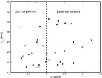
Fig. 4. The difference between the predicted and observed transit times to 1 AU (1τ) against solar wind speed upstream of the ICME. Positive (negative) values of1τ correspond to ICMEs that arrive earlier (later) than predicted. The solid horizontal line shows the average upstream solar wind speed of 427 km/s. There does not appear to be any correlation between the late/early arrival of ICMEs and the upstream solar wind speed.
each CME and (c) the point of intersection of the spacecraft and the ICME, as inferred from observations of the sheath region.
4.1 CME speed at the Sun
When the location of the CME source on the solar surface is known (from X-ray or EUV observations), a simple geomet-ric correction can be applied to the plane of sky speed to infer the radial speed if the CME width is known. (Of course, it needs to be stated that such corrections are subject to errors due to the fact that the X-ray activity can be located any-where under the CME; e.g. Harrison, 1986.) Gopalswamy et al. (2001a) assumed an average CME width of 72◦, but found the error between the predicted and observed transit times in-creased when the corrected speeds were used. It should be noted that the average width of 72◦ covers a wide range of values, thus the error introduced by assuming that all CMEs have the same angular width is greater than that introduced by the projection effect. A further difficulty with correcting for projection effects is the difficulty in relating the observed halo CME with matter actually moving earthwards. While simple cosine projections are commonly used, more sophisti-cated models may be needed to give the correct radial speeds (e.g. Zhao et al., 2002).
Bearing in mind these caveats, two methods of assessing the error introduced by the projection effect in predictingτ are investigated in this study. The first is to use a data set for which projection to both speed and transit time is absent: i.e. the quadrature observations of CME – ICME pairs. The effective interplanetary acceleration (a2: shown in Fig. 1) for these 19 events is given by Eq. (9) and is the effective
ac-celeration averaged to a distance of 0.76 AU (the average he-liocentric distance at which the in situ measurements were made). Thus, at heliocentric distances greater or less than 0.76 AU, it is unsurprising that predictions of transit time based upon this parameter are highly inaccurate: for the 19 quadrature observations (made at a range of heliocentric dis-tances from 0.63 to 0.92 AU) the average error inτ is 0.54 days for the G2000 model, and 0.55 for the G2001 model, in agreement with the estimates of Gopalswamy et al. (2001).
The VG2002 model does not use an effective total accel-eration, but is based on the assumption that the deceleration of the ICME at any heliocentric distance is proportional to its speed relative to the ambient solar wind. Using best-fit parameters ofα = −0.002,β =1.48 andWo =524 km/s obtained for this set of observations, the average error inτ is 0.46 days, comparable to the non-quadrature observations (0.41 days). The best-fit aerodynamic drag coefficients for the quadrature and E-S line observations are also similar, but the quadrature observations require a significantly higher so-lar wind speed (524 km/s compared to 438 km/s). It should be noted that due to the small number of events, the phase-space minima used to locate the best-fit parameters is quite broad (e.g. constrainingWoto a more reasonable 438 km/s still allows a fit to be achieved whereby the average error in τ is 0.52 days). For this reason we do not make any physical interpretation of the best-fit parameters.
As a second method for assessing the speed projection ef-fect, we use the VG2002 model, but with the ICME speed at 1 AU speed as the sole input parameter, and integrate back to the Sun, and compare the time the CME was predicted to have left the Sun with the actual onset time there. This ef-fectively removes the plane of sky projection error from the estimate of transit time. For the 35 E-S line events, this gave <|1τ|>=0.38 days (compared to 0.41 days with the pro-jection). Hence, the removal of the projection effect yields only a minor improvement (∼0.03 days) in the prediction accuracy of the transit time. These two results, coupled with the findings of Gopalswamy et al. (2001a), lead us to con-clude that projection effects are not the major cause of the error in the transit times.
4.2 Solar wind conditions
−1 −0.5 0 0.5 1 1.5 5
10 15 20 25 30 35 40 45
∆τ (days)
Average ICME |B| (nT)
Later than predicted Earlier than predicted
Fig. 5.The average magnetic field intensity of an ICME as a func-tion of1τ (predicted – actualτ). Late arriving ejecta have lower magnetic field intensities than early ones.
The ambient solar wind speed encountered by an ICME is defined as the average solar wind speed for 12 h upstream of the ICME-driven shock front, or upstream of the leading edge of the ICME for cases when a shock was not present. Different definitions of the ambient solar wind speed (e.g. 1 h to 1 day upstream averages) do not greatly affect our results. The solar wind speed (Vsw) experienced by the 35 E-S line ICMEs ranged from 324 km/s to 647 km/s, with an average of 427 km/s. For a CME withU =800 km/s, an increase in solar wind speed from 324 to 647 km/s would decrease the value ofτ predicted by the VG2002 model from 4.3 days to 2.5 days. Thus, the variation inVswis potentially significant. Figure 4 shows the difference between the predicted and observed transit time to 1 AU (1τ is negative for those ICMEs arriving later than predicted, positive for early) as a function of the solar wind speed. One would expect that higher solar wind speeds would lead to earlier arrivals, and lower speeds to later arrivals. In fact, there does not appear to be any correlation between1τ and the solar wind speed. A similar lack of correlation was found for solar wind den-sity and ram pressure (not shown). The net drag experienced by the ICME should depend on the ratio of the ICME to so-lar wind density, so that a denser soso-lar wind would lead to a delayed arrival and vice versa. However, we note that in the VG2002 model, this density ratio is included in the best-fit parametersaandβ.
Furthermore, using the observed values ofVsw as the pa-rameterWoin model C in fact increases<|1τ|>to approx-imately 0.6 days (compared to 0.41 days when all ICMEs are assumed to be embedded in an identical solar wind of speed 438 km/s).
−1 −0.5 0 0.5 1 1.5
0.2 0.4 0.6 0.8 1 1.2 1.4 1.6 1.8
∆τ (days)
Sheath Duration (days)
Later than predicted Earlier than predicted
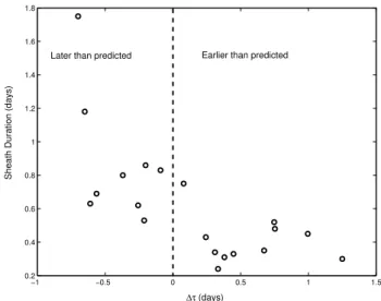
Fig. 6. Sheath region duration as a function of the difference be-tween the predicted and actual transit time to 1 AU (1τ).
4.3 The role of the ICME magnetic field
The drag force will tend to equalise the speed of the ICME and solar wind, and clearly this is important in determining the observed speed of ICMEs at 1 AU. However, the flux rope nature of many ICMEs (e.g. magnetic clouds) implies that in some topologies there can be a significant outward Lorentz force (e.g. Chen, 1996). Thus, one should look for a corre-lation between early arrival and the average ICME magnetic field strength. In addition, as we shall discuss in Sect. 4.4, information about how1τ depends on the field strength can yield clues to which part of an ICME one is encountering. In both cases, one would expect stronger fields to be associ-ated with earlier arrivals. The result of such a study using the VG2002 model is shown in Fig. 5. There is a weak trend towards early arrival for stronger field strengths (the late ICMEs have an average magnetic field strength of 10.2 nT, while early ones have an average field of 14.8 nT). However, it should be noted that even using extremes of the distribu-tion (i.e. the means of|B|for ejecta with1τ = ±0.3 days), we could only discount the null hypothesis with an 80% con-fidence.
4.4 Properties of the ICME sheath region
du-0 200 400 600 800 0
10 20 30 40 50 60
Vmax (km/s)
|B|
max
(nT)
−2000 0 200 400 600 800 1000
10 20 30 40 50 60
Sheath region. ICME.
Fig. 7.The relationship betweenVmaxand|B|max, (Vmax-Vsw) and (|B|max) shown as “o”s (“+”s) for the sheath region and ICME body.
ration of 0.41 days and a thickness of 1.9×10⁷km. Thus, combining this with the results of the previous section, late arriving ICMEs have both thicker sheath regions and lower magnetic field intensities.
4.5 Predicting the magnetic field intensity at 1 AU
Prediction of the arrival time and velocity of an ICME at 1 AU is only the first step in space weather forecasting. The intensity of any triggered geomagnetic storm is dependent upon the ICME’s geo-effectiveness, which is determined by its velocity, and especially by the strength and duration of any southward IMF, both within the ICME itself and the pre-ceding sheath region.
Previous studies have shown the existence of a linear re-lationship between maximum speed (Vmax) and maximum magnetic field intensity (|B|max) of magnetic clouds (Gon-zalez et al., 1998) Subsequently Owens and Cargill (2002) showed that such a relationship extended to all periods of the solar wind with a high magnetic field intensity (typically above 18 nT for a period of 3 h). Here we re-investigate this relation between magnetic field intensity and speed for the 35 E-S line ICMEs at 1 AU. For ICMEs that drive shocks, the relation is analysed for both the sheath region and the ICME itself, as defined in Sect. 2. The results are shown in Fig. 7, with crosses and circles representing the absolute speed and speed relative to the upstream solar wind of the ICME, respectively. Table 3 gives details of the linear best-fit parameters: the correlation is strong between the maxi-mum speed relative to the solar wind and the maximaxi-mum mag-netic field intensity of the sheath region. However, we find a much weaker relationship between magnetic field inten-sity and speed within the body of the ICME, but note that two-thirds of the ICMEs used in this study had peak field intensities below the 18 nT threshold found by Owens and Cargill (2002) to give significant correlation.
Table 3.The relations between maximum field intensity and maxi-mum speed, and maximaxi-mum field intensity and maximaxi-mum speed rel-ative to the upstream solar wind are given for both the sheath region and ICME body for the 35 E-S line ICMEs. The linear best fit pa-rameters (in the form|B| = mV +c),χ2 and linear correlation coefficient (r) are given.
Linear Best Fit (|B| =mV+c)
m c χ2 r
Sheath |B|- (Vmax−Vsw) 0.080 12.12 0.017 0.81
|B| −Vmax 0.040 1.38 0.027 0.67
ICME |B| −(Vmax-Vsw) 0.041 10.99 0.036 0.56
|B| −Vmax 0.037 -3.91 0.027 0.51
4.6 Interpretation
It is clear that little improvement in estimating ICME arrival time can be expected from efforts to model the effects dis-cussed in Sect. 4.1 and 4.2. The lack of dependence on the projection angle suggests that either halo CMEs are struc-tures that exhibit some sort of spherical symmetry, so that the velocity seen in the plane of the sky is approximately the same as that directed earthwards, or that if there is not ex-act spherical symmetry, the difference in the component of velocity directed Earthwards from the total velocity is small. Indeed recent results using LASCO data from Michalek et al. (2003) for an extensive sample of halo CMEs originating away from Sun-centre indicate that the difference between the plane of the sky and actual speeds may differ by only 20%.
They concluded that the discrepancy between the model and the observations increased when the CME speeds were cor-rected for possible plane-of-sky projection by using a simple geometry and an average cone angle for all CMEs. However, our null results suggest that projection is not the major cause of the observed spread in 1 AU transit times. Furthermore, the azimuthal expansion speed of a halo CME, as measured by a coronagraph at the L1 point, appears to be a good proxy for the radial speed of a CME along the E-S line, and hence, may be an adequate input for this class of models.
The lack of dependence on the ambient solar wind speed is surprising since it is clear that the relative motion between the ICME and solar wind is an important factor in determin-ing the ICME speed, and the associated aerodynamic drag force will depend on the relative speed. It is unlikely that this is a result of single-point measurements of the solar wind. Solar wind structures usually extend over a significant frac-tion of a CME size.
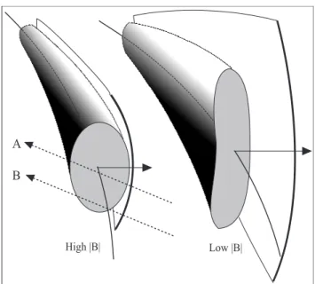
The only quantity studied that showed a significant cor-relation with the error in the transit time was the thickness of the sheath ahead of the ICME, although there was also a weak correlation with the magnetic field strength. In fact, these results have mutual explanations, as shown in Fig. 8. The observed sheath thickness ahead of an ejecta is deter-mined by both the physical properties of the ICME (espe-cially its speed, since slower CMEs will have wider, but weaker sheaths) and the point of observation. One explana-tion focuses on the spatial properties characteristic of plasma sheaths associated with moving objects. The thickness of a sheath ahead of the main part of the ICME is known to in-crease with distance from the nose of a curved ICME (Rus-sell and Mulligan, 2002); thus, a spacecraft intersecting an ICME away from the nose should see a wider sheath coupled with a longer apparent transit time than one flying through the middle. This is sketched in the left part of Fig. 8, where spacecraft A goes through the centre of the ICME, seeing a narrow sheath, while spacecraft B goes through the edge, and sees a broader sheath. For the same ICME, spacecraft A would report an earlier ICME arrival than spacecraft B, consistent with the tendency for late arrivals to be associated with a thicker sheath. This scenario can also account for the trends in the ICME magnetic field intensity. The magnetic field strength within a magnetic cloud falls off with distance away from the axis, where the axis is here defined as being along the direction of the ICME toroidal field (see Fig. 8). Thus, a late-arriving event would also see a reduced mag-netic field intensity as the spacecraft passed through the edge of the ICME. Thus, we believe that the spread inτ could be due to a geometric effect.
A second possible explanation of the results in Sects. 4.3 and 4.4 arises from the result of recent numerical simulations (e.g. Vandas et al., 1995; Cargill et al., 2000), which indicate that the degree of deformation of the cross-sectional shape of an ICME by the solar wind depends upon the magnetic field intensity and topology within the ICME. This is illus-trated in the right-hand part of Fig. 8, where an ICME with a weak magnetic field has undergone additional lateral
expan-Fig. 8. A representation of possible ICME cross sections at 1 AU for high|B|and low|B|events. In the former case the string field leads to the ICME maintaining an approximately circular cross sec-tion, while for a weaker field, the ICME becomes elongated in the vertical direction in this sketch. The arrow denotes the direction of ICME motion, the curved line ahead of the ICME corresponds to a possible bow shock location and the solid line coming out of the body of the CME corresponds to a schematic axis of the ICME. Two possible spacecraft crossings are shown for the high|B|picture: A passing close to the central axis, and B clipping the outer edge of the ICME.
sion. This lateral expansion will lead to an increase in the aerodynamic drag force (Cargill et al., 1995, 2000), and so a later arrival time. The wider, slower moving ICME will also have a thicker sheath region.
4.7 Discussion
Our results appear to suggest that CME velocities at the Sun measured in the plane of the sky are adequate for ICME prediction, provided, of course, one can associate these with a halo event, and that a simple solar wind model is adequate. However, one can expect STEREO observations to give a better determination of the velocity vector of the CME at the Sun, and it is easy with an L1 monitor to use real-time ambient solar wind data. But for forecasting the ICME ar-rival time, the L1 solar wind parameters are not essential (of course, they are essential for understanding what effect the ICME has on the magnetosphere and ionosphere).
An important new measurement would be enhanced pre-cision in the direction of ICME propagation. This would enable one to not only improve the ICME arrival time, as we have noted in this paper, but also to make a prediction about its geo-effectiveness. An ICME that strikes a “glanc-ing blow” at the Earth will not only lead to a weaker IMF (see Sect. 4.6), but also any interval of southward IMF will be shorter (Cargill et al., 1994). The forthcoming STEREO mission provides an excellent opportunity to see if realistic estimates of ICME propagation can really lead to significant improvements in space weather forecasting.
Finally, we note that the perennial difficulty with predict-ing the magnetic field strength of an ICME remains unre-solved. Although our earlier work showed good correlations between the solar wind velocity and maximum field strength for events with a maximum field>18 nT, the correlation is actually weaker when one restricts the analysis to ICMEs. This is due to a dominance of events with lower magnetic fields, a possible consequence of “off-axis” ICME crossings (i.e. path B in Fig. 8). However, the correlation between speed and magnetic field intensity is significant relative to the solar wind speed in the sheath region. This relation could be the result of draping of the solar wind magnetic field in front of the faster moving ICME. Thus, though prediction of solar wind speed at 1 AU may not be required to predict the arrival time of ICMEs, it is needed to forecast the magnetic properties of the sheath region.
Acknowledgements. We acknowledge support from PPARC and
QuinetiQ. We have benefited from the availability of ACE data at NSSDC, in particular the MAG (P.I. N. Ness) and SWEPAM (P.I. D. McComas) instruments. The CME catalogue is generated and maintained by NASA and The Catholic University of America in cooperation with the Naval Research Laboratory. SOHO is a project of international cooperation between ESA and NASA. We would also like to thank Adam Rees for useful discussions.
The Editor in Chief thanks two referees for their help in evalu-ating this paper.
References
Brueckner, G. E., Howard, R. A., Koomen, M. J., Korendyke, C. M., Michels, D. J., Socker, D. G., Dere, K. P., Lamy, P. L., Lle-baria, A., Bout, M. V., Schwenn, R., Simnett, G. M., Bedford, D. K., and Eyles, C. J.: The large angle spectroscopic coronagraph (LASCO), Sol. Phys., 162, 357, 1995.
Burlaga, L. F.: Magnetic clouds: Constant alpha force-free config-urations, J. Geophys. Res., 93, 7217, 1988.
Cargill, P. J., Chen, J., Spicer, D. S., and Zalesak, S. T.: The de-formation of flux tubes in the solar wind with applications to the structure of magnetic clouds and CMEs, Proc. of the Third SOHO Workshop, 291, 1994.
Cargill, P. J., Chen, J., Spicer, D. S., and Zalesak, S. T.: Geometry of interplanetary magnetic clouds, Geophys. Res. Lett., 22, 647, 1995.
Cargill, P. J., Chen, J., Spicer, D. S., and Zalesak, S. T.: MHD simulations of the motion of magnetic flux tubes through a mag-netized plasma, J. Geophys. Res., 101, 4855, 1996.
Cargill, P. J., Schmidt, J., Spicer, D. S., and Zalesak, S. T.: The magnetic structure of over expanding CMEs, J. Geophys. Res., 105, 7509, 2000.
Chen, J.: Effects of toroidal forces in current loops embedded in a background plasma, Astrophys. J., 338, 453, 1989.
Chen, J.: Theory of prominence eruption and propagation: inter-planetary consequences, J. Geophys. Res., 101, 27 499, 1996. Daglis, I. A.: Space storms, ring current and space-atmosphere
cou-pling, NATO ASI Space Storms and Space Weather Hazards, Kluwer Publishers, 2001.
Gonzalez, W. D., Clua De Gonzalez, A. L., Dal Lago, A., Tsuru-tani, B. T., Arballo, J. K., Lakhina, G. S., Buti, B., and Ho, G. M.: Magnetic cloud field intensities and solar wind velocities, Geophys. Res. Lett., 25, 963, 1998.
Gopalswamy, N.: Relation between CMEs and ICMEs, in: “Solar-terrestrial Magnetic Activity and Space Environment”, COSPAR Colloquia Series, 14, edited by Wang, H. N. and Xu, R. L., p. 157, 2002.
Gopalswamy, N., Lara, A., Lepping, R. P., Kaiser, M. L., Berdichevsky, D., and St. Cyr, O. C.: Interplanetary acceleration of coronal mass ejections, Geophys. Res. Lett., 27, 145, 2000. Gopalswamy, N., Lara, A., Yashiro, S., Kaiser, M. L., and Howard,
R. A.: Predicting the 1-AU arrival times of coronal mass ejec-tions, J. Geophys. Res., 106, 29 207, 2001a.
Gopalswamy, N., Yashiro, S., Kaiser, M. L., Howard, R. A., and Bougeret, J.-L.: Radio signatures of coronal mass ejection inter-action: Coronal mass ejection cannibalism?, Astrophys. J., L91, 548, 2001b.
Harrison, R. A.: Solar coronal mass ejections and flares, Astron. Astrophys., 162, 283, 1986.
Howard, R. A., Michels, D. J., Sheely, N. R., and Koomen, M. J.: The observation of a coronal transient directed at Earth, Astro-phys. J. Lett., 263, 101, 1982.
Hundhausen, A. J.: Coronal mass ejections, in : The many faces of the Sun, edited by Strong, K. T., Springer Press, p. 143. 1999. Lagarias, J. C., Reeds, J. A., Wright, M. H., and Wright, P. E.:
Convergence Properties of the Nelder-Mead Simplex Method in Low Dimensions, SIAM Journal of Optimization, 9, Number 1, 112, 1998.
Lindsay, G. M., Luhman, J. G., Russell, C. M., and Gosling J. T.: Relationships between coronal mass ejection speeds from coro-nagraph images and interplanetary characteristics of associated interplanetary coronal mass ejections, J. Geophys. Res., 104, 12 515, 1999.
McComas, D. J., Bame, S. J., Barker, S. J., Feldman, W. C., Phillips, J. L., Riley, P., and Griffee, J. W.: Solar wind electron proton alpha monitor (SWEPAM) for the Advanced Composition Ex-plorer, Space Sci. Rev., 86, 563, 1998.
mass ejections, Astrophys. J., 584, 472, 2003.
Owens, M. J. and Cargill, P. J.: Correlation of magnetic field in-tensities and solar wind speeds of events observed by ACE, J. Geophys. Res., 107, 1050, 2002.
Phillips, J. L., Bame, S. J., Barnes, A., Barraclough, B. L., Feld-man, W. C., Goldstein, B. E., Gosling, J. T., Hoogeveen, G. W., McComas, D. J., Neugebauer, M., and Suess, S. T.: Ulysses so-lar wind plasma observations from pole to pole, Geophys. Res. Lett., 22, 3301, 1995.
Russell, C. T. and Mulligan, T.: On the magnetosheath thicknesses of interplanetary coronal mass ejections, Planetary and Space Sci., 50, 527, 2002.
St. Cyr., O. C., Howard, R. A., Sheely, Jr., N. R., Plunkett, S. P., Michels, D. J., Paswaters, S. E., Koomen, M. J., Simnett, G. M., Thompson, B. J., Gurman, J. B., Schwenn, R., Webb, D. F., Hild-ner, E., and Lamy, P. L.: Properties of coronal mass ejections: SOHO LASCO observations from January 1996 to June 1998, J. Geophys. Res., 105, 18 169, 2000.
Sheeley, N. R., Jr., Wang, Y. M., Hawley, S. H., Brueckner, G. E., Dere, K. P., Howard, R. A., Koomen, M. J., Korendyke,
C. M., Michels, D. J., Paswaters, S. E., Socker, D. G., St. Cyr, O. C., Wang, D., Lamy, P. L., Llebaria, A., Schwenn, R., Simnett, G. H., Plunkett, S. and Biesecker, D. A.: Measrements of the flow speed in the corona between 2 and 30rs, Astrophys.
J., 484, 472, 1997.
Smith, C. W., L’Heureux, J., Ness, N. F., Acuna, M. H., Burlaga, L. F., and Scheifele, J.: The ACE magnetic fields experiment, Space Sci. Rev., 86, 613, 1998.
Vandas, M., Fischer, S., Dryer, M., Smith, Z., and Detman, T.: Sim-ulation of magnetic cloud propagation in the inner heliosphere in two-dimensions: 1. loop perpendicular to the ecliptic plane, J. Geophys. Res., 100, 12 285, 1995.
Vrˇsnak, B. and Gopalswamy, N.: Influence of aerodynamic drag on the motion of interplanetary ejecta, J. Geophys. Res., 107, 10.1029/2001/JA000120, 2002.