The eect of the high-speed stream following the corotating
interaction region on the geomagnetic activities
S. Watari
Communications Research Laboratory, 4-2-1 Nukuikita, Koganei, Tokyo 184, Japan
Received: 3 July 1996 / Received: 20 January 1997 / Accepted: 13 February 1997
Abstract.The high-speed stream following the corotat-ing interaction regions (CIRs) was analyzed. As a result of the analysis, it is found that the geomagnetic ®eld is continuously disturbed in the high-speed stream in question. The geomagnetic disturbances with long duration recurred several rotations between December 1993 and June 1994. These disturbances were associated with a large recurrent coronal hole expanding from the south pole of the Sun. High-speed solar wind from this coronal hole was observed by the IMP-8 satellite during this period. However, the observed intensities of the geomagnetic disturbances were dierent for each recur-rent period. This is explained by the seasonal eect. The disturbed geomagnetic condition continued in the high-speed stream after the passage of the CIRs. The long duration of these disturbances can be explained by the continuous energy input into the Earth's magnetosphere from the high-speed regions following the CIRs. This kind of long-duration geomagnetic disturbance in asso-ciation with coronal holes has been observed in the declining phase of other solar cycles. The relation between the coronal-hole area and the maximum solar-wind velocity is not good for the well-developed large coronal hole analyzed here.
1 Introduction
Some geomagnetic disturbances recur with about a 27-day period during several solar rotations. Bartels (1934) gave the name M-regions to the solar sources of these recurrent geomagnetic disturbances. Now it is generally accepted that these 27-day recurrent geomagnetic dis-turbances are associated with corotating interaction regions (CIRs) formed between the high-speed solar wind emanating from coronal holes and the preceding slow solar wind. This is based on the results of several spacecraft observations (Neupert and Pizzo, 1974; Timothy et al., 1975; Nolte et al., 1976; Bohlin and
Sheeley, 1978; Broussard et al., 1978; Sheeley et al., 1976).
Nolteet al.(1976) noted that the velocity of the solar wind from coronal holes is roughly proportional to the area of the holes, and the holes located near the equator have more chance of aecting the Earth than polar ones. However, the recent analysis by Watari et al. (1995) showed that the relation between coronal-hole area and solar-wind velocity is more complicated than that derived by Nolteet al.(1976).
The recurrent disturbances caused by the CIRs are most remarkable during the declining phase of solar cycles when the coronal holes are largest and extend to the solar equator (Sheeley and Harvey, 1981; Watari, 1990).
According to Joselyn (1995), on average only 20% of the observed near-equatorial coronal holes (located within 30° of the helioequator) are associated with
geomagnetic storms (Ap index ³30; the Ap index is a planetary averaged daily geomagnetic index). Thomson (1995a, b) also noted a poor correlation (£0.10) between
individual coronal-hole parameters (e.g., area, polarity, and latitude) and Apindex.
To explain their results, we also have to consider the eect of the propagation between the Sun and Earth and the eect of coupling between solar wind and the magnetosphere as well as the coronal-hole parameters.
Considering the eect of propagation, it is dicult quantitatively to measure or estimate the following eect: the formation of southward interplanetary mag-netic ®eld (IMF) and high dynamic pressure in the CIRs during the propagation.
solar wind from the coronal hole is dominant (Phillips
et al., 1994, 1995).
Considering the coupling eect, many researchers (Garrettet al., 1974; Burtonet al., 1975; Iyemoriet al., 1979; Akasofu, 1981; Baker, 1986; Fay et al., 1986; McPherron et al., 1986; Murayama, 1986; Feldstein, 1992; Price and Prichard, 1993) have studied on this subject. One problem is the nonlinear response of the magnetosphere (Klimas et al., 1996 and references therein); Vassiliadis et al. (1995) used the nonlinear ®ltering to describe it, and other researchers (Lundstedt, 1992; Lundstedt and Wintoft, 1994; Gleisner et al., 1996) applied the neural network to this problem. However, there is still room for improvement.
With respect to the seasonal dependence of the coupling eect, Sheeley and Harvey (1981) pointed out the presence of Russell-McPherron eect (Russell and McPherron, 1973) on the CIRs. Crooker and Cliver (1994, and references therein) and Crookeret al.(1996) noted the important role of the Russell-McPherron eect on both coronal streamers and CIRs. Joselyn (1995) noted that coronal holes of either polarity can be associated with storms throughout the year even though there is a tendency for negative polarity holes to be more geoeective in the spring (February±April) and positive polarity holes to be more geoeective during August± October. This suggests that both propagation and coupling eects are important in estimating the relation between coronal-hole characteristics and the size of geomagnetic storms.
Recently, Lindsay et al. (1995) studied the statistics of solar-wind parameters, which were observed by the Pioneer Venus Orbiter (PVO) between 1979 and 1988, in coronal mass ejections (CMEs) and CIRs. They found that both CIRs and CMEs produce magnetic ®elds signi®cantly larger than the normal IMF. The CIRs are often associated with the ¯uctuating north-south com-ponent (Bz) of the IMF and tend to produce larger dynamic pressures than the CMEs. According to Tsurutani et al. (1995a, and references therein), the increase of the IMF ¯uctuation is due to large-amplitude AlfveÂn waves within the body of the corotating streams. Ulysses also observed the large-amplitude IMF ¯uctu-ations in the high-speed stream (Tsurutaniet al., 1995b). There are many studies on the CIRs and their eect on the geomagnetic disturbances mentioned already. However, the eect of high-speed regions following the CIRs on the geomagnetic disturbances has never been fully examined before. There is a query as to how the high-speed regions after the passage of the CIRs aect the geomagnetic condition. Here, the above subject is discussed using the long-duration recurrent geomagnetic storms observed between December 1993 and June 1994. The Dst index is used as an indicator of geomagnetic disturbances in this study. The index is a measure of variation in the geomagnetic ®eld due to the equatorial ring current. It is calculated from the horizontal components at approximately four near-equatorial geo-magnetic stations at hourly intervals. The relation between this index and solar-wind parameters is ex-plained physically (Feldstein, 1992, and references
therein). Burton et al. (1975) noted that there is an empirical relationship between the Dst index and solar-wind parameters [e.g., velocity (V), the north-south component of the IMF (Bz), and mass density (q); the solar-wind electric ®eld (VBz) and the dynamic pressure (q V2/2)].
2 Observation
Between December 1993 and June 1994 (Bartels rotation number 2910±2916), long-duration geomagnetic distur-bances recurred several rotations associated with a large negative-polarity coronal hole extending from the south pole of the Sun [P. Lantos (Observatoire de Paris-Meudon), private communication, 1994; Watari, 1995]. During this period, several satellite anomalies are reported in association with high-energy electrons. Baker et al. (1994, 1996) related these high-energy electrons with the high-speed stream from the well-developed coronal hole.
After the Skylab era the HeI 10830-nm line at Kitt Peak National Observatory was used to distinguish coronal holes. Since late 1991 there has been continuous solar observation by the Japan/US soft X-ray telescope (SXT) (Tsuneta et al., 1991) on board the Yohkoh
satellite. HeI coronal holes are usually associated with the soft X-ray ones. However, the HeI coronal holes are smaller than the soft X-ray coronal holes and they show patchy structure (Watari et al., 1995). This perhaps re¯ects the expansion of the magnetic ®eld in the coronal hole because HeI observes in lower solar atmosphere than soft X-ray. Here the SXT images are used to recognise coronal holes. Coronal holes are observed as a dark area in soft X-ray images because of their low density.
Figure 1 shows the time evolution of a coronal hole observed by the SXT between December 1993 and April 1994. The dark region extending from the south pole in the soft X-ray images is a coronal hole with negative polarity. This large well-developed coronal hole re-curred during several rotations shown in Fig. 1. The white curves in Fig. 1 show the boundary of the coronal hole determined by the soft X-ray intensity.
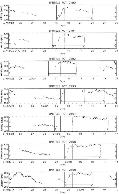
Figure 2 shows the 1-h-averaged solar-wind velocity observed by the IMP-8 satellite during this period. The arrows in Fig. 2 note the periods of ³500 km/s solar
wind in association with the southern coronal hole in Fig. 1. To examine further the eect of the recurrent streams, they are divided into CIRs (regions between two vertical solid lines shown in Fig. 2) and high-speed regions (HSRs: regions between two vertical dashed lines in Fig. 2) following the CIRs. Here, CIRs and HSRs are de®ned as below. CIRs are the regions with the density enhancement in the solar wind by compres-sion between slow and fast solar wind. HSRs are the regions with ³500 km/s solar-wind speed after the CIR
passage. There is a good correspondence between the southern coronal hole and the observed high-speed solar wind (see Figs. 1 and 2).
lines, and the vertical dashed lines in Fig. 3 correspond with those in Fig. 2. The disturbed geomagnetic condi-tion continued after the passage of the CIRs, or in the HSRs. According to Figs. 2 and 3, the observed Dst variations were dierent even though the high-speed solar wind was observed associated with the coronal hole. This suggests that it is dicult to relate directly the coronal-hole parameters with the geomagnetic activities (Thomson, 1995a, b). The geomagnetic activities asso-ciated with the negative-polarity southern coronal hole are stronger and longer between February and April.
3 Statistical analysis
Table 1 summarizes the periods ofV³ 500 km/s of the
solar wind associated with the south coronal hole with negative polarity, the maximum solar-wind velocity, and the ratios of the maximum velocity to background solar-wind velocity (see the periods noted by the arrows in Fig. 2). Here, the low-speed solar wind in front of the CIRs is considered as the background solar wind. This table also shows the observed southern coronal hole areas between the helioequator and 30° south from it
Fig. 1. Evolution of coronal holes observed by the soft X-ray telescope (SXT) on board the Japanese Yohkoh satellite. Thewhite curvesin the ®gure show the boundaries of the coronal holes determined by soft X-ray intensity
Table 1. Periods of high-speed streams associated with coronal holes, maximum solar-wind velocities, ratios of maximum to background solar-wind velocity, maximum Dst indices, and coronal-hole areas between the helioequator and 30°south of it. (Vback: background solar-wind velocity; *: aected by data gaps.)
Bartels rotation ³500 km/s solar wind Max. velocity Vmax/Vback Max. Dst Hole area between 0
start (UT) end (UT) Vmax (km/s) (nT) and S30°(109km2)
2190 93/12/16/0700 93/12/22* 710 2.09 )44 2.6
2191 94/01/11/1300 94/01/17* 775 2.58 )42 4.0
2192 94/02/06* 94/02/17* 805 )126 7.9
2193 94/03/07/0900 94/03/20/0500 775 2.13 )109 7.7
2194 94/04/06* 94/04/13* 839 2.23* )111 10.0
2195 94/05/01/1900 94/05/10* 824 2.05* )79 4.0
(see Fig. 1) and the maximum Dst index during the recurrent geomagnetic disturbances in association with the coronal hole (see the periods noted by the arrows in Fig. 3). The coronal-hole areas were determined based on the soft X-ray images shown in Fig. 1.
High-speed streams with maximum velocity above 700 km/s were observed associated with the large well-developed recurrent coronal hole for every rotation during this period. However, the relation between the coronal-hole area and the observed maximum velocity is not good (see Table 1). This result supports the recent
result by Watari et al. (1995), and might suggest saturation, because all high-speed streams selected here exceed 700 km/s at their maximum speed. Usually a high-speed stream associated with coronal holes does not exceed 850 km/s at Earth.
The eect on geomagnetic disturbances (see maxi-mum Dst index in Table 1) was dierent for each Bartels rotation. The interesting point is that the largest maximum Dst index in Table 1 is not associated with the highest maximum velocity and the largest coronal hole. The observed maximum velocities and Dst indices
Fig. 2. Solar-wind velocity observed by IMP-8 between December 1993 and June 1994
are dierent even though the coronal holes are approx-imately same size (4.0´ 109km2). The observed
max-imum Dst index in the Table 1 shows a larger value around March for the high-speed streams with approx-imately same maximum velocity (775 km/s).
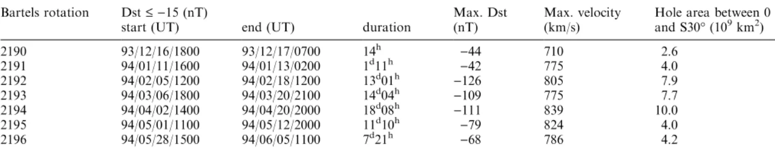
Table 2 shows the start, end, and duration of disturbed geomagnetic condition (Dst£ )15) in
associ-ation with the high-speed stream from the south-pole coronal hole. The observed coronal-hole area and the maximum velocity dier for each Bartels rotation. However, it seems that the duration becomes longer in March and April.
Figure 4 shows the distribution of velocity (V), number density (n), temperature (T), north-south com-ponent of IMF (Bz) in GSE and GSM, total ¯ux of IMF (jBj), solar-wind electric ®eld (VBz) in GSE and in GSM, dynamic pressure (qV2/2) in the CIRs between Decem-ber 1993 and June 1994 (Fig. 4a), in the HSRs (b), and in both the CIRs and the HSRs (c). The distribution is calculated for all 1-h-averaged data in the periods noted by the vertical solid lines (a), the vertical dashed lines (b), and the arrows (c) in Fig. 2.
Mass density (q) is given by mpn and mp is proton mass. Two coordinate systems are used for Bz. One is
the geocentric solar-ecliptic (GSE) coordinate system. The other is the geocentric solar magnetosphere (GSM) coordinate system. Bz is perpendicular to the ecliptic plane in the GSE and parallel to the dipole axis of the Earth in the GSM. Bz in GSM minimizes the Russell-McPherron eect when we estimate the coupling eect betweenBzand the magnetosphere.
Table 3 gives the average values and the standard deviations of solar-wind parameters. In CIRs and
HSRs, the average value of Bz in GSM was about ten times larger than that in GSE. In CIRs, the average value ofjVBzjin GSM was about eight times larger than that in GSE. In HSRs, the average value of jVBzj in GSM was about twenty times larger than that in GSE. In CIRs, the average values ofn,jBj, and deviation of
jBj were large (see Fig. 4b), because the interaction between slow- and high-speed streams produces turbu-lent conditions in CIRs. The velocity gradually
in-Fig. 4. aDistribution of solar-wind parameters in all the observed data.bDistribution of solar-wind parameters in the HDRs.cDistribution of solar-wind parameters in the HSRs
Table 2. Periods of Dst index of £)15 nT associated with coronal holes, maximum Dst indices, maximum solar-wind velocities, and coronal-hole areas between the helioequator and 30°south of it
Bartels rotation Dst£)15 (nT) Max. Dst Max. velocity Hole area between 0
start (UT) end (UT) duration (nT) (km/s) and S30°(109km2)
2190 93/12/16/1800 93/12/17/0700 14h )44 710 2.6
2191 94/01/11/1600 94/01/13/0200 1d11h
)42 775 4.0
2192 94/02/05/1200 94/02/18/1200 13d01h )126 805 7.9
2193 94/03/06/1800 94/03/20/2100 14d04h )109 775 7.7
2194 94/04/02/1400 94/04/20/2000 18d08h
)111 839 10.0
2195 94/05/01/1100 94/05/12/2000 11d10h )79 824 4.0
2196 94/05/28/1500 94/06/05/1100 7d21h
)68 786 4.2
creased in these regions (see Fig. 2). The larger electric ®eld and dynamic pressure in the CIRs could control the magnitude of geomagnetic disturbances. The strong magnetic ®eld with large ¯uctuation in the CIRs may reduce the seasonal dependence. The high dynamic pressure in the CIRs strongly compresses the magneto-sphere and disturbs the geomagnetic ®eld. This could also reduce the seasonal dependence.
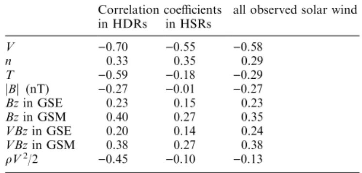
Table 4 shows the correlation coecient between Dst indices and 1-h-averaged solar-wind parameters by the IMP-8 satellite in the CIRs, the HSRs, and both the CIRs and HSRs. All 1-h-averaged values in the periods noted by the arrows in Figs. 2 and 3 are used in calculating the correlation. The IMP-8 satellite is in near-circular 35-Earth radii orbit and the 1-h-averaged solar-wind parameters are used here. Hence, the dier-ence of the location between the IMP-8 satellite and the magnetopause is neglected in the analysis. Bzand VBz
in GSM show better correlation than in GSE. This suggests the Russel-McPherron eect in both CIRs and HSRs. However, overall correlation between Dst indices and solar-wind parameters was very low except for velocity. The highest correlation ()0.7) is with the velocity in CIRs.
4 Concluding remarks
The long-duration geomagnetic disturbances between December 1993 and June 1994 are analyzed. These disturbances are associated with the well-developed southern coronal hole. This recurrent hole was associ-ated with high-speed solar wind of above 700 km/s during this period. However, the size (magnitude and duration) of the geomagnetic disturbances was dierent for each rotation. It was found that the disturbed geomagnetic condition continues in the high-speed streams following the CIRs. They have the potential to keep a disturbed geomagnetic condition.
The coupling between the interplanetary magnetic ®eld and geomagnetic ®eld controls the magnitude and period of disturbed geomagnetic condition. The corre-lation between the Dst index and solar-wind parameters was low (less than 0.5), except for velocity. The average values of nand jBjand deviation of jBj were larger in the CIRs because of compression (Lindsay et al., 1995). In CIRs, the Dst index showed good correlation with dynamic pressure. This is an explanation for the weak seasonal dependence of polarity of coronal holes in association with geomagnetic disturbances (Joselyn, 1995). In the HSRs, larger VBz due to high velocity seems continuously to disturb the geomagnetic ®eld. Watari (1990), Tsurutani et al. (1995a), and Crooker
Table 4. Correlation coecients between Dst indices and solar-wind parameters in the HDRs, HSRs, and all observed solar solar-wind
Correlation coecients all observed solar wind in HDRs in HSRs
V )0.70 )0.55 )0.58
n 0.33 0.35 0.29
T )0.59 )0.18 )0.29
jBj (nT) )0.27 )0.01 )0.27
Bzin GSE 0.23 0.15 0.23
Bzin GSM 0.40 0.27 0.35
VBzin GSE 0.20 0.14 0.24
VBzin GSM 0.38 0.27 0.38
qV2/2 )0.45 )0.10 )0.13 Table 3. Average values and standard deviations of solar-wind
parameters in HDRs, HSRs, and all observed solar wind
in HDRs in HSRs all observed solar wind
V(km/s) 559 145 705 65 581 136
n(cm-3) 11.8 6.2 4.0 1.1 6.2 4.7
T(MK) 0.24 0.18 0.18 0.10 0.14 0.13
jBj(nT) 8.2 3.9 4.9 1.2 5.6 2.8
Bzin GSE (nT) )0.08 3.72 )0.06 1.71 0.17 2.52 Bzin GSM (nT) )0.91 3.65 )0.55 1.80 0.09 2.81 VBzin GSE (mV) 0.07 1.41 0.02 2.12 )0.06 1.22 VBzin GSM (mV))0.59 2.08 )0.40 1.22 )0.02 1.57
qV2/2 (nPa) 2.80 1.26 1.64 0.36 1.58 1.67
et al. (1996) noted the long duration geomagnetic disturbances in the declining phases of other solar cycles.
The relation between the coronal-holes area and maximum solar-wind speed is not good in this analysis. This might suggest saturation, because well-developed coronal holes are analyzed here.
Acknowledgments.This work was done as part of the Japan-France cooperation program. The author thanks Dr. P. Lantos (Obser-vatoire de Paris-Meudon) for his suggestions and encouragement in this work. I thank NOAA/NGDC for Dst data, NASA/NSSDC for the IMP-8 data, and Yohkoh SXT-team for soft X-ray images. Topical Editor R. Schwenn thanks S. Bravo and another referee for their help in evaluating this paper.
References
Akasofu, A. -I.,Energy coupling between the solar wind and the magnetosphere,Space Sci. Rev.,28,121, 1981.
Baker, D. N., Statistical analyses in the study of solar wind-magnetosphere coupling, inSolar wind-magnetosphere coupling, Eds. Y. Kamide and J. A. Savin, Terra Scienti®c Publishing, Tokyo, pp. 17±38, 1986.
Baker, D. N., S. Kanekal, J. B. Blake, B. Klecker, and G. Rostoker,
Satellite anomalies linked to electron increase in magneto-sphere,EOS,75,401, 1994.
Baker, D. N.,High-energy electrons in earth's magnetosphere: their eects and methods of prediction, in Proc. Solar-Terrestrial Prediction Workshop,Hitachi,Japan, in press, 1997.
Bartels, J., Twenty-seven day recurrences in terrestrial magnetic and solar activity,J. Geophys. Res.,37,1, 1934.
Bohlin, J. D., and N. R. Sheeley Jr.,Extreme ultraviolet observa-tions of coronal holes,Solar Phys.,56,125, 1978.
Broussard, R. M., N. R. Sheeley Jr., R. Tousey, and J. H. Under-wood,A survey of coronal holes and their solar-wind associations throughout sunspot cycle 20,Solar Phys.,56,161, 1978.
Burton, R. K., R. L. McPherron, and C. T. Russell,An empirical relationship between interplanetary condition and Dst, J. Geophys. Res.,80,4204, 1975.
Crooker, N. U., and E. W. Cliver,Postmodern view of M-regions,
J. Geophys.Res.,99,13383, 1994.
Crooker, N. U., A. J. Lazarus, R. P. Lepping, K. W. Ogilvie, J. T. Steinberg, A. Szabo, and T. G. Onsager,A two-stream, four-sector, recurrence pattern: implications from WIND for the 22-year geomagnetic activity cycle,Geophys. Res. Lett.,23, 1275, 1996.
Fay, R. Y., C. R. Garrity, R. L. McPherron, and D. N. Baker,
Prediction ®lters for the Dst index and the polar-cap potential, inSolar wind-magnetosphere coupling, Eds. Y. Kamide and J.A. Savin, Terra Scienti®c Publishing, Tokyo, pp. 111±118, 1986.
Feldstein, Y. I.,Modelling of the magnetic ®eld of magnetospheric ring current as a function of interplanetary medium parameter,
Space Sci. Rev.,59,83, 1992.
Garrett, H. B., A. J. Dessler, and T. W. Hill,In¯uence of solar wind variability on geomagnetic activity,J. Geophys. Res.,79,4603, 1974.
Gleisner, H., H. Lundstedt, and P. Wintoft,Predicting geomagnetic storms from solar-wind data using time-delay neural networks,
Ann. Geophysicae,14,679, 1996.
Gosling, J. T., S. J. Bame, D. J. McComas, J. L. Philips, V. J. Pizzo, and B. E. Goldstein,Latitudinal variation of solar wind corotating stream interaction regions: Ulysses, Geophys. Res. Lett.,20,2789, 1993.
Iyemori, T., H. Maeda, and T. Kamei, Impulse response of geomagnetic indices to interplanetary magnetic ®elds, J. Ge-omagn. Geoelectr.,31,1, 1979.
Joselyn, J. A., Geomagnetic activity forecasting: the state of the art,Rev. Geophys.,33,383, 1995.
Klimas, A. J., D. Vassiliadis, D. N. Baker, and D. A. Roberts,The organized nonlinear dynamics of the magnetosphere, J. Geo-phys. Res.,101,13089, 1996.
Lindsay, G. M., C. T. Rusell, and J. G. Luhmann,Coronal mass ejection and stream interaction region characteristics and their potential geomagnetic eectiveness, J. Geophys. Res., 100,
16999, 1995.
Lundstedt, H.,Neural networks and predictions of solar-terrestrial eects,Planet. Space Sci.,40,457, 1992.
Lundstedt, H., and P. Wintoft, Prediction of geomagnetic storms from solar-wind data with the use of a neural network, Ann. Geophysicae,12,19, 1994.
McPherron, R. L., D. N. Baker, and L. F. Bargatze,Linear ®lters as a method of real-time prediction of geomagnetic activity, in
Solar wind-magnetosphere coupling, Eds. Y. Kamide and J. A. Savin, Terra Scienti®c Publishing, Tokyo, pp. 85±92, 1986.
Murayama, T.,Coupling function between the solar wind and the Dst index, inSolar wind-magnetosphere coupling, Eds. Y. Ka-mide and J. A. Savin, Terra Scienti®c Publishing, Tokyo, pp. 119±126, 1986.
Neupert, W. M, and V. Pizzo, Solar coronal holes as sources of recurrent geomagnetic disturbances, J. Geophys. Res., 79,
253701, 1974.
Nolte, J. T., A. S. Krieger, A. F. Timothy, R. E. Gold, E. C. Roelof, G. Vaiana, A. J. Lazarus, J. D. Sullivan, and P. S. McIntosh,
Coronal holes as sources of solar wind, Solar Phys., 46, 303, 1976.
Phillips, J. L., A. Baloph, S. J. Bame, B. E. Goldstein, J. T. Gosling, J. T. Hoeksema, D. J. McComas, M. Neugebauer, N. R. Sheeley Jr., and Y.-M. Wang,Ulysses at 50°south: constant immersion in the high-speed solar wind, Geophys. Res. Lett., 21, 1105, 1994.
Phillips, J. L., S. J. Bame, W. C. Feldman, J. T. Gosling, C. M. Hammond, D. J. McComas, B. E. Goldstein, and M. Ne-ugebauer, Ulysses solar-wind plasma observations during the declining phase of solar cycle 22,Adv. Space Res.,16,85, 1995.
Pizzo, V. J.,The evolution of corotating stream fronts near the ecliptic plane in the inner solar system, 2. Three-dimensional tilted-dipole fronts,J. Geophys. Res.,96,5405, 1991.
Pizzo, V. J., and Gosling, J. T., 3D simulation of high-latitude interaction regions: comparison with Ulysses results,Geophys. Res. Lett.,21,2063, 1994.
Price, C. P., and D. Prichard, The nonlinear response of the magnetosphere: 30 October 1978,Geophys. Res. Lett.,20,771, 1993.
Riley, P., J. T. Gosling, L. A. Weiss, and V. J. Pizzo,The tilts of corotating interaction regions at midheliographic latitudes,
J. Geophys. Res.,101,24349, 1996.
Russell, C. T., and R. L. McPherron, Semiannual variation of geomagnetic activity,J. Geophys. Res.,78,92, 1973.
Sheeley Jr., N. R. and J. W. Harvey,Coronal holes, solar wind streams, and recurrent geomagnetic disturbances during 1978 and 1979,Solar Phys.,70,237, 1981.
Sheeley Jr., N. R., J. W. Harvey, and W. C. Feldman, Coronal holes, solar wind streams, and geomagnetic disturbances: 1973± 1976,Solar Phys.,49,271, 1976.
Thomson, A. W. P.,Coronal hole observations and the prediction of the Ap geomagnetic index, Proc. IUGG XXI General Assembly, pp. B168, 1995a.
Thomson, A. W. P.,A statistical relationship between coronal hole central meridian passage, J. Geomagn. Geoelectr., 47, 1263, 1995b.
Timothy, A. F., A. S. Krieger, and G. S. Vaiana,The structure and evolution of coronal holes,Solar Phys.,42,135, 1975.
Tsuneta, S., L. Acton, M. Bruner, J. Lemen, W. Brown, R. Cara-valho, S. Freeland, B. Jurcevich, M. Morrison, Y. Ogawara, T. Hirayama, and J. Owens,Soft X-ray telescope for the Solar-A mission,Solar Phys.,136,37, 1991.
Tsurutani, B. T., W. D. Gonzalez, A. L. C. Gonzalez, F. Tang, J. K. Arballo, and M. Okada,Interplanetary origin of geomagnetic activity in the declining phase of the solar cycle,J. Geophys. Res.,100,21717, 1995a.
Tsurutani, B, T., C. M. Ho, J. K. Arballo, B. E. Goldstein, and A. Balogh, Large-amplitude IMF ¯uctuations, in corotating interaction regions: Ulysses at midlatitude,Geophys. Res. Lett.,
22,3397, 1995b.
Vassiliadis, D., A. J. Klimas, D. N. Baker, and D. A. Roberts,A description of the solar wind-magnetosphere coupling based on nonlinear ®lters,J. Geophys. Res.,100,3495, 1995.
Watari, S., The latitudinal distribution of coronal holes and geomagnetic storms due to coronal holes, Proc. 1989 Solar-Terrestrial Prediction Workshop, Edited by R. T. Thomp-son, D. G. Cole, P. J. WilkinThomp-son, M. A. Shea, D. Smart, G. Heckman. Published by National Oceanic and Atmos-pheric Administration, Environmental Research Laboratories, Boulder, Colorado, Leura, Australia,1,627, 1990.
Watari, S., Soft X-ray coronal holes and interplanetary distur-bances,Proc. IUGG Gen. Assem., pp. B168, 1995.