www.ann-geophys.net/24/1085/2006/ © European Geosciences Union 2006
Annales
Geophysicae
Ionospheric and boundary contributions to the
Dessler-Parker-Sckopke formula for
Dst
V. M. Vasyli ¯unas
Max-Planck-Institut f¨ur Sonnensystemforschung, 37191 Katlenburg-Lindau, Germany
Received: 21 September 2005 – Revised: 10 February 2006 – Accepted: 14 February 2006 – Published: 19 May 2006
Abstract. The Dessler-Parker-Sckopke formula for the dis-turbance magnetic field averaged over the Earth’s surface, universally used to interpret the geomagneticDstindex, can be generalized, by using the well known method of deriv-ing it from the virial theorem, to include the effects of iono-spheric currents. There is an added term proportional to the global integral of the vertical mechanical force that balances the vertical component of the Lorentz forceJ×B/cin the ionosphere; a downward mechanical force reduces, and an upward increases, the depression of the magnetic field. If the vertical component of the ionospheric Ohm’s law holds exactly, the relevant force on the plasma is the collisional friction between the neutral atmosphere and the vertically flowing plasma. An equal and opposite force is exerted on the neutral atmosphere and thus appears in its virial theo-rem. The ionospheric effect onDstcan then be related to the changes of kinetic and gravitational energy contents of the neutral atmosphere; since these changes are brought about by energy input from the magnetosphere, there is an implied upper limit to the effect on Dst which in general is rela-tively small in comparison to the contribution of the plasma energy content in the magnetosphere. Hence the Dessler-Parker-Sckopke formula can be applied without major mod-ification, even in the case of strong partial ring currents; the ionospheric closure currents implied by the local time asymmetry have only a relatively small effect on the glob-ally averaged disturbance field, comparable to other sources of uncertainty. When derived from the virial theorem ap-plied to a bounded volume (e.g. the magnetosphere bounded by the magnetopause and a cross-section of the magneto-tail), the Dessler-Parker-Sckopke formula contains also sev-eral boundary surface terms which can be identified as contri-butions of the magnetopause (Chapman-Ferraro) and of the magnetotail currents.
Keywords. Magnetospheric physics (Magnetosphere-ionosphere interactions; Solar wind-magnetosphere interac-tions; Storms and substorms)
Correspondence to:V. M. Vasyli¯unas ([email protected])
1 Introduction
The Dessler-Parker-Sckopke theorem gives the magnetic field perturbation at the Earth due to plasma trapped in the terrestrial dipole magnetic field and is therefore of funda-mental importance in relating the geomagneticDst index to the properties of plasma in the magnetosphere. Written in modern notation, their formula is
µ·b(0)=2UK (1)
whereµis the dipole moment,b(0)is the magnetic distur-bance field, nominally evaluated at the center of the Earth but also equal to the (vector) average over the surface of the globe, andUK is the total kinetic energy content of plasma
in the magnetosphere. Equation (1) was derived (Dessler and Parker, 1959) by summing the currents associated with the gradient, curvature, and magnetization drifts of plasma par-ticles trapped in a dipole magnetic field (assuming linearity and axial symmetry: drifts in an unperturbed field, uniform distribution in longitude), at first for two special distributions (isotropic and flat) of pitch angles and later (Sckopke, 1966) for arbitrary pitch angle distributions. Subsequently several groups (Maguire and Carovillano, 1967; Baker and Hurley, 1967; Carovillano and Maguire, 1968; Olbert et al., 1968) gave a simpler, rigorous derivation by an argument related to the virial theorem, without the restrictive assumptions of linearity and axial symmetry, generalizing the formula to
µ·b(0)=2UK+Ub (2)
whereUbis the total energy content in the disturbance
mag-netic field: Ub=
Z
drb2/8π b≡B−Bdipole (3)
earlier derivations that effectively treated the magnetosphere as extending to infinity). The entire development has been definitively reviewed by Carovillano and Siscoe (1973).
Although the Dessler-Parker-Sckopke theorem might thus seem to be a closed chapter at least as far as theory is con-cerned, there still are some outstanding issues which are ad-dressed in this paper:
1. First and foremost, there remains at least one fundamen-tal problem: none of the existing derivations known to me have included ionospheric currents, which are potentially im-portant particularly for configurations with strong local-time asymmetries (closure of “partial ring currents”) and have sometimes (e.g. Liemohn et al., 2001; Liemohn, 2003) been adduced as a reason for questioning the applicability of the theorem. Whathasbeen done by many authors (e.g. Parker, 1966; Siscoe and Crooker, 1974; Crooker and Siscoe, 1974, 1981; Friedrich et al., 1999; Munsani, 2000, and others) is to calculate, on the basis of some specific model, the magnetic effects of a complete asymmetric current system (e.g., partial ring current or substorm current wedge), including the iono-spheric closure together with all the other currents. However useful such model results may be in their particular context, it is not clear how they are to be combined with the Dessler-Parker-Sckopke formula; for instance, should the kinetic en-ergy of plasma in the partial ring current be included in the UK term of Eqs. (1) and (2)?
2. The entire theoretical development beyond the origi-nal papers of Dessler and Parker (1959) and Sckopke (1966) still seems to be little known and poorly understood. The boundary surface terms in particular are almost universally ignored (or sometimes misunderstood; see discussion in Ap-pendix A), boundary effects onDstbeing taken into account by ad hoc “corrections” instead. On a more basic level, it is hardly ever appreciated that the Dessler-Parker-Sckopke theorem, although formally equivalent to the Biot-Savart law (Vasyli¯unas, 2001) and of course originally derived by ap-plying it, has a physical basis quite distinct from (and more restrictive than) the Biot-Savart law.
In this paper I present, in Sect. 2, a rigorous and gen-eral derivation of the Dessler-Parker-Sckopke formula from the virial theorem, taking into account ionospheric effects, bounded volume, and also time-derivative terms (neglected from the start in most discussions). In Sect. 3, I evaluate the ionospheric contributions and show that they are relatively small and can for most purposes be neglected in practice. In Sect. 4, I consider the boundary surface terms and their relation to the usual, empirically derived, pressure correc-tions and magnetotail current contribucorrec-tions. The end result (Sect. 5) is a version of the Dessler-Parker-Sckopke expres-sion forDst that is formally complete and contains all the relevant terms, with each term unambiguously defined and all terms derived, in a uniform consistent fashion, from clearly identified physical premises.
Two important aspects, concerning applications of the Dessler-Parker-Sckopke theorem rather than the theorem
it-self, are beyond the scope of this paper and will not be dealt with. First, the conversion between the nominal disturbance fieldb(0)that appears in the theorem and theDstindex that is determined from observations (e.g., Chapter 8 of Mayaud, 1980, and references therein) is here treated as given en-tirely by the conventionally used scaling factor, with at most passing mention of the implied assumptions and outstand-ing problems. Second, the use of the theorem for studyoutstand-ing magnetospheric and geomagnetic-storm dynamics, in partic-ular for predictingDsttime series on the basis of solar-wind and other inputs, is a separate topic and constitutes an ex-tensive field of research in its own right (e.g. Burton et al., 1975; O’Brien and McPherron, 2000, 2002; McPherron and O’Brien, 2001; Liemohn et al., 2001, 2002; Jordanova et al., 1998, 2003; Siscoe et al., 2005a,b, and many others); else-where (Vasyli¯unas, 2006) I discuss how the magnetotail term derived here affects some prediction equations forDst.
2 Derivation from the virial theorem
The virial theorem in general uses the momentum equation (taking its dot product with the radius vector and integrating by parts) to infer global constraints on the various energies within the system under consideration. (Simplest and best-known example: in a stable self-gravitating system, potential energy plus twice kinetic energy equals zero.) In the particu-lar application that leads to the Dessler-Parker-Sckopke the-orem, the momentum equation that now includes the Lorentz forceJ×B/cis subjected to the procedure described above, followed by special manipulation in order to isolate the mag-netic disturbance field in the region near the magmag-netic dipole. The mathematical derivation is presented in detail below, but the following physical point may be noted at the outset. The essential physical basis of the Dessler-Parker-Sckopke theo-rem is the assumed validity of the momentum equation; when the theorem is derived from the Biot-Savart law, the currents that appear in the Biot-Savart integral are those determined by the requirement thatJ×B/cbalance the rest of the mo-mentum equation. It is in this sense that, as noted in the in-troduction, the Dessler-Parker-Sckopke theorem is more re-strictive than the Biot-Savart law. (This is also the reason why combining terms from the Dessler-Parker-Sckopke for-mula with disturbance fields calculated from model currents not constrained by the momentum equation is always prob-lematic.)
2.1 Formal derivation
The starting point for the virial theorem is the momentum equation of the plasma
(∂/∂t ) (ρV)+∇·T=ρg+f (4) whereTis the total stress tensor
electric field terms have been neglected (assumption of quasi-neutrality and VA2≪c2), gravity is for our purposes
more conveniently included as the term ρg on the right-hand side, although it could be added to T instead (see, e.g., Siscoe, 1970), andf represents all other forces not in-cluded inT, in particular plasma-neutral collisions important in the ionosphere. (For a discussion of the virial theorem in a more general gravitational-hydromagnetic context, see Chandrasekhar, 1961, Chapter XIII, section 117).
Consider a volume bounded by a closed inner surface and a closed outer surface; the boundaries are to be precisely de-fined later but can be thought of as, roughly, the Earth and the magnetopause, respectively. Taking the dot product of Eq. (4) with the radius vectorr, integrating over the volume under consideration, and using the identity
(∇·T)·r =∇·(T·r)−Trace(T) (6) together with the relation between the trace of a stress tensor and the corresponding energy density yields
(d/dt ) Z
drρV·r+
Z
dS·T·r=
2UK+UB+UG+
Z
dr f ·r (7)
where the surface integrals are over the boundaries of the volume; UK andUB represent the volume integrals of the
kinetic energy density (including bulk flow and thermal en-ergies) of the plasma and the energy density of the (total) magnetic field, respectively:
UK =
Z
dr (1/2)ρV2+Trace(P) UB=
Z
dr B2/8π . (8)
The gravitational termUGrepresents the integral
UG=
Z
drρg·r (9)
which may in the present case, with the Earth excluded from the volume of integration and with g approximated as the spherically symmetric gravity field of the Earth (neglecting any non-symmetric terms as well as self-gravity of the mass within the volume), be viewed as the gravitational energy; note that it differs from the gravitational terms in the for-mulations of Chandrasekhar (1961) or Siscoe (1970), where these approximations are not made. The termUG is always
negative and may be treated as simply a reduction ofUKby
an amount that, in the case of plasma, is easily shown to be negligible.
The first term on the left-hand side of Eq. (7) can be refor-mulated by invoking the relations
ρV·r =ρV ·∇r2/2
=∇·ρVr2/2−r2/2∇·ρV
=∇·ρVr2/2+(∂/∂t ) ρr2/2 (10)
where the last line follows from mass continuity; Eq. (7) can then be rewritten as
1
2
d2/dt2 Z
drρr2+ Z
dS·h(∂ρV/∂t ) r2/2+T·ri
= 2UK+UB+UG+
Z
dr f·r (11) (cf. Rossi and Olbert, 1970, Problem 10.1). The integral in the first term on the left-hand side of Eq. (11) looks like (and is often described as) the moment of inertia of the system, which is not quite accurate because the radius vector in it is measured from an arbitrary origin rather than from the cen-ter of mass. By introducing, however, the cencen-ter of massR through the definitions
MR≡
Z
drρr M≡ Z
drρ (12) it is possible to further rewrite Eq. (11), after extensive ma-nipulation, as
1
2d 2I/dt2
+
Z
dS·h(∂ρV/∂t )|r−R|2/2+T·(r−R)i
= 2UK−M
R˙
2
+UB+UG∗ +
Z
dr f ·(r−R) (13) where
UG∗ = Z
drρg·(r−R) (14) and
I≡
Z
drρ|r−R|2=
Z
drρr2−R2 (15) is the properly defined moment of inertia; everything is now referred to the center of mass as the origin, and the kinetic en-ergy of motion of the system as a whole has been subtracted. Elegant though it may be, Eq. (13) as distinct from Eq. (11) is important only for systems subject to external forces suf-ficiently strong and asymmetric to produce appreciable ac-celeration of the system as a whole. For the magnetosphere anchored to the massive Earth this is certainly not the case, and throughout this paper I shall use Eq. (11) withr mea-sured from the center of the Earth.
The essential application of the virial theorem is to sys-tems that endure, that do not undergo either fast dispersion or fast collapse. The first term on the left-hand side of Eq. (11) or (13) (the second time derivative of the moment of inertia) can then be neglected, and balance of the remaining terms is the condition for the system to endure. Equivalently, if e.g. the (positive) energiesUKandUBwere not balanced by
2.2 Steps toward the Dessler-Parker-Sckopke relation To obtain the Dessler-Parker-Sckopke relation from the virial theorem, two steps are needed. First, choose as the lower boundary of the volume of integration the surface of a small Earth-centered sphere (of radiusRs∼RE), at which only the magnetic terms in the stress tensor are assumed significant. (For the later purpose of estimating the ionospheric contribu-tions, it will be important that the surface lie below the iono-sphere.) Evaluating the surface term at the lower boundary then transforms Eq. (11) into
−Rs3
R
dhB2/8π− B· ˆr2/4πi
= 2UK+UB+UG (16)
−R
dS·h(∂ρV/∂t ) r2/2+T·ri+
Z
dr f ·r where the surface integral on the right-hand side refers only to the upper boundary, the integral R
d over the lower boundary having been transferred to the left-hand side. Sec-ond, replace the momentum Eq. (4) by the corresponding equation containing a curl-free magnetic fieldBd alone and
no plasma,
∇·hIBd2/8π
−BdBd/4π
i
=0 , (17)
and carry out the same procedure (dot product withr, inte-gration over the assumed volume) to obtain the counterpart of Eq. (16):
−Rs3
Z
dhBd2/8π− Bd· ˆr
2 /4πi
=UBd−
Z
dS·hrBd2/8π
−(BdBd/4π )·r
i
(18) where
UBd ≡
Z
dr Bd2/8π (19)
AlthoughBd, as its designation suggests, will soon be
iden-tified as the dipole field, the only property ofBd invoked
so far is that, within the volume under consideration, it has zero curl and hence can be written as the gradient of a scalar potential,Bd= −∇ψ.
Now subtract Eq. (18) from Eq. (16). The difference of the magnetic energies can be written as
UB −UBd = Ub+
Z
dr b·Bd/4π
=Ub−
Z
dr b· ∇ψ/4π (20)
=Ub−
Z
dS· bψ/4π+Rs3
Z
db· ˆrψ/4π
where Ub andb have been defined in expression (3). The
third term in the last line of Eq. (20) can be transferred to
the left-hand side of the difference equation, Eq. (16) minus Eq. (18), which then becomes
−Rs3
Z
dnb·
Bd− ˆr 2Bd· ˆr−ψ/Rs
/4π
+hb2−2 b· ˆr2i/8πo. (21) Assume now thatBdis indeed the dipole field. Then
Bd·r =2ψ=2µ· ˆr/r2 (22)
and the quantity in [ ] in the first line of expression (21) can be rewritten as
−∇ψ−3ψ rˆ/r= −r−3∇r3ψ= −µ/r3 (23) evaluated atr=Rs; the second line of expression (21) can be
neglected to orderb/Bd. Finally, the left-hand side of the
difference equation, Eq. (16) minus Eq. (18), becomes Z
(d/4π ) µ·b=µ·b(0) . (24) 2.3 Expression for the disturbance field
With all this taken into account, and with the assumption of a gyrotropic pressure tensor, Eq. (16) minus Eq. (18) can be written, after some manipulation, as
µ·b(0)=2UK+Ub+UG+
Z
dr f ·r (25)
−
Z
dS·rhP⊥+B2/8πi
+
Z
dS·[Bd×(r×Bd)]/8π
+
Z
dS·B[χB−(Bd/2)]·r/4π
−
Z
dS·h(∂ρV/∂t ) r2/2+ρV(V ·r)i
where the factorχ≡1−
long as the outer boundary lies within the magnetosphere) is related to bulk flow through the boundary. Note the signs of the various terms;µ·b(0)>0 corresponds toDst <0.
The presence of the purely dipole-field expression in the third line and of the subtracted dipole field in the second term of the fourth line might seem somewhat peculiar. A formal check, however, on the correctness of Eq. (25) can be made by setting all the plasma terms to zero andB to the dipole field everywhere within the volume; then the only non-zero terms are the three surface integrals in lines 2, 3, and 4 (with B=Bd,P⊥=0, andχ=1), and they must add up to zero –
as they indeed do, but only thanks to these “peculiar” terms! The expression in the third line can be evaluated explicitly (by redefining the normal direction as pointing inward and invoking the curl-free property ofBd) and shown to equal
the energy density of the dipole field integrated over the vol-umeexternalto the outer boundary. The significance of this becomes apparent upon comparing Eq. (25) with the corre-sponding earlier result of Siscoe (1970, his Eq.(23)):
µ·b(0)=2UK+Ub∗−
Z
dS·rhP⊥+B2/8πi (26) in our notation. (This equation was derived also from the virial theorem, by a slightly different but equivalent method: Siscoe (1970) takes the virial of a volume that includes the Earth and then subtracts the virial of the Earth, while I take from the start a volume that excludes the Earth.) Lines 4 and 5 of Eq. (25) are absent because Siscoe (1970) explicitly as-sumed the magnetosphere to be closed, with no field or flow across the magnetopause, and also he did not consider any ionospheric effects. What still needs to be explained is the absence in Eq. (26) of line 3 of Eq. (25). The reason lies in the different definitions of the energy of the disturbance field:Ubin Eq. (25) is the integral over the volume between
the inner and the outer surface, whileUb∗in Eq. (26) is the
integral over all space. The two thus differ by the energy of the disturbance field integrated over the volume beyond the outer surface; for the closed magnetosphere assumed by Sis-coe (1970), the disturbance field beyond the magnetopause is equal to minus the dipole field.
3 Ionospheric contribution
The ionospheric contribution to the dipole-aligned compo-nent of the disturbance field at the center of the Earth, given by the termRdr f·rin Eqs. (7), (11), (16), or (25), is pro-portional to the integral, over the entire ionosphere, of radial force density times radial distance. This dependence can be easily understood by noting that the Biot-Savart integral over the current distribution for thezcomponent of the field at the origin can be written (cf. Eq. (A7) of Vasyli¯unas, 2001) as
bz(0)=
Z
dr sinθ/r2φˆ·J/c (27)
and thatµsinθ/r2is simplyrBθ of the dipole field;
multi-plied by the dipole moment, the integrand is thusr·J×B/c, the radial component of the Lorentz force which must be bal-anced by the sum of all the non-magnetic forces. The pres-sure gradient and flow acceleration forces do not appear ex-plicitly, nor does gravity; they have been included already as part of the total energy integralUK and the gravitational
termUG, respectively. The remaining “other force”f in the
ionosphere is just the plasma-neutral collisional friction: f = −νinρ (V−Vn) (28)
whereVnis the bulk flow velocity of the neutral atmosphere
andνin is the ion-neutral collision frequency (electron
col-lision effects on the plasma momentum equation being neg-ligible over most of the ionosphere, except at the lowest al-titudes). The expression for the partδb(0)I contributed by
the ionospheric term in the Dessler-Parker-Sckopke formula then is
µ·δb(0)I =
Z
dr f ·r = −
Z
dr νinρ (V −Vn)·r ,
(29) proportional to the global integral of the collisional frictional force due to the differentialverticalbulk flow of the plasma relative to the neutral atmosphere.
3.1 Role of the neutral atmosphere
One might be tempted to assume that the ionosphere is for the most part gravitationally bound and hence the vertical com-ponent off must be small compared to gravity; this would imply an upper limit to µ·δb(0)I of order UG, negligibly
small in comparison to the contributionUKof the plasma
en-ergy content in the magnetosphere. The vertical component, however, of the Lorentz forceJ×B/cfor typical values of the auroral electrojet, whether up or down (up for eastward, down for westward electrojet), can easily be estimated and shown to exceed by some orders of magnitude the gravita-tional forceρgon the plasma alone; it still is small, however, compared toρ(n)g, the gravitational force on the neutral at-mosphere. Clearly, the ionosphere is held in place by the neu-tral atmosphere, not by its own weight. The forcef on the plasma is matched by an equal and opposite force on the neu-tral medium; that all the magnetic stresses on plasma in the ionosphere are transferred, via plasma-neutral collisions, en-tirely to the neutral atmosphere is in fact an essential assump-tion underlying the convenassump-tional ionospheric Ohm’s law (Va-syli¯unas and Song, 2005). The termR
drf·rin Eq. (29) also appears therefore, with opposite sign, in the virial theorem for the neutral atmosphere, the neutral-medium counterpart of Eq. (11):
−Rs3
Z
d P(n)= 2UK(n)+UG(n)− Z
where the superscript(n)identifies quantities referring to the neutral atmosphere; the surface integrals have been evalu-ated under the assumption that at the outer boundary all sur-face terms are negligible and at the inner boundary only the pressure is significant (all the magnetic terms are of course absent).
With the use of Eq. (30), the ionospheric contribution to the Dessler-Parker-Sckopke formula may be expressed as
µ·δb(0)I =
Rs3
Z
d P(n)
+2UK(n)+UG(n). (31) The right-hand side of Eq. (31) contains terms that are very large (by magnetospheric standards) but, being both positive and negative, very nearly cancel each other. If, for exam-ple,RSis chosen to correspond to altitude 100 km where the
atmospheric pressure is 0.3 dynes cm−2, the contribution of the first term (effect of pressure at the inner boundary, nu-merically equal to twice the kinetic energy content within the volumeinwardof the boundary if the pressure there were held constant at its boundary value) alone would give aDst value of −1.27 Gauss (−1.27×10⁵nT); it is balanced, of course, by +1.27 Gauss from the third term. The second term is smaller than the third (this is the condition that the atmosphere be gravitationally bound) by about the ratio (at-mospheric scale height/Earth radius), but it would still con-tribute about −400 nT to Dst. In short, the terms on the right-hand side add up to very nearly zero, by the dynamics of the neutral atmosphere alone, and the magnetic effects rep-resent only a very small perturbation on that. It is therefore more meaningful to rewrite Eq. (31) as
µ·δb(0)I =
Rs3
Z
d δP(n)
+2δUK(n)+δUG(n) (32) where theδ’s are the changes of the various neutral ener-gies that occur in association with magnetic disturbances. As these can be positive or negative, it is convenient to in-troduce a single symbol1U(n) to represent the net change of the relevant energy content of the neutral atmosphere, al-lowing Eq. (32), the ionospheric contribution toDst, to be finally expressed as
µ·δb(0)I =
Z
dr f ·r ≈ 1U(n). (33) There does not seem to be any general method of evaluat-ing1U(n)other than integrating a complete global model for f·r (in which caseµ·δb(0)I might as well be calculated
di-rectly from Eq. (27)). Some significant constraints on1U(n) may, however, be imposed by considerations of energy trans-fer between the magnetosphere and the neutral atmosphere. 3.2 Magnetospheric perturbations of the neutral
atmo-sphere
Two effects of magnetospheric processes on the neutral at-mosphere are well known. The first is heating, both by direct
heat flux from the magnetosphere (in the form of charged-particle precipitation) and by dissipation resulting from elec-trodynamic processes. The latter is commonly referred to as “ionospheric Joule heating” but Vasyli¯unas and Song (2005) have shown that it is, for the most part, collisional fric-tional heating from the relative motion of plasma and neu-trals; the conventionally used expressionJ· E+V(n)×B/c does, however, represent the total dissipation rate, about half of which goes into the neutral medium. The second process is acceleration of neutral flow by ion drag (e.g. Song et al., 2005, and references therein).
Neither one of these processes, however, is directly con-nected with the ionospheric effect onDst. Heating increases the pressure and hence the kinetic energy content, but it also changes, through vertical displacements produced by the pressure imbalance, the gravitational potential energy con-tent; the two come into equilibrium, satisfying Eq. (32) with zero on the left-hand side, on a time scale of a sound wave crossing a scale height (minutes or less). Ion drag affects the neutral atmosphere flow only on long time scales, an hour or more at typical ionospheric altitudes. Clearly, only those changes on the right-hand side of Eq. (32) that aredirectly re-lated to the vertical component of the Lorentz forceJ×B/c in the ionosphere are relevant toDst.
For the purpose of describing the effect of the vertical magnetic stresses exerted from the magnetosphere, the mo-mentum equation for the neutral medium can be written in a form that explicitly includes the Lorentz force,
(∂/∂t )ρ(n)V(n)+∇·ρ(n)V(n)V(n)+ ∇P(n)
=ρ(n)g+J×B/c , (34) by noting that the neutral-ion collision term is equal to mi-nus the ion-neutral collision term in the momentum equation for ionospheric plasma and hence to the Lorentz force which the latter balances. Taking the divergence of Eq. (34) and in-voking the continuity equation gives a wave equation for the neutral density changeδρ(n), with∇·J×B/cas the source term,
∂2/∂t2δρ(n)+∇·cs2∇δρ(n)
−g· ∇δρ(n)
=∇·J×B/c , (35)
where only terms linear in the perturbation amplitude have been kept; cs2 is the speed of sound. If δρ(n) initially is
zero everywhere and the Lorentz force turns on att=0, the spatial-gradient terms are at first negligible and the density will initially change as∼t2,
δρ(n)≈ −t2/2∇ ·J×B/c≈t2/2B· ∇ ×J/c
≈ t2/2Bθ (∂/∂r) Jφ/c (36)
follows from the fact that vertical variation of horizontalJ is the dominant contribution to∇×J. Because the density is changing, the gravitational force also changes, coming into balance with the Lorentz force when
δρ(n)g· ˆr ≈ −ˆr·J×B/c≈Bθ Jφ/c (37)
i.e. after a timeτ given approximately by
gτ2/2 (∂/∂r)log|Jφ| ≡gτ2/2λ∼ ±O (1) . (38)
This is equal to the free-fall time across the typical verti-cal sverti-caleλof the current density profile. The value ofλis determined primarily by the scale height of the neutral at-mosphere (at altitudes above the maximum current density) and by the fall-off of the electron concentration (at altitudes below ). Typically,λ∼some tens of kilometers, givingτ∼ minutes; inclusion of changes in pressure gradient in addition to gravitational force would modify this estimate somewhat, but not in order of magnitude.
We thus have a remarkable result: the neutral atmosphere, usually viewed as responding to magnetospheric plasma flows only on a time scale of hours, can nevertheless ad-just itself in minutes in order to balance vertical magnetic stresses imposed from the magnetosphere. (This is possible because the requisite changes of the neutral density are very small compared to the density itself.) But it is precisely the global integral of these vertical stresses which represents the ionospheric contribution toDst. Hence the primary contri-bution to1U(n)is the change of gravitational potential en-ergy in Eq. (32), given by the globally integrated, asymp-totic long-time (t≫τ) limit of the density change described by Eq. (36). The changes of the pressure and kinetic-energy terms may, by comparison, be neglected: the associated adi-abatic changes are smaller by the square of the ratio (sound speed/gravitational escape speed), while the non-adiabatic (heating) changes proceed independently and, as discussed above, establish their own gravitational equilibrium without magnetic effects.
3.3 Magnitude of the ionospheric contribution
The ionospheric term1U(n)in the Dessler-Parker-Sckopke formula is thus equal to a fraction, not precisely specified but expected in general to be small, of the total energy supplied from the magnetosphere to the atmosphere. That energy, in turn, is comparable to the total energy supplied to the in-ner magnetosphere and the ring current, although the precise partitioning is a matter of some controversy (e.g. Weiss et al., 1992; Koskinen and Tanskanen, 2002; Feldstein et al., 2003, and references therein). In any case,1U(n)should be small in comparison to the plasma kinetic energy termUKand can
for most purposes be neglected. (UKincludes the kinetic
en-ergy of all the plasma within the volume under consideration; no distinctions, e.g., between symmetric and partial ring cur-rents or between ring current and other particle populations, are made.)
Note that the above result is an upper limit on the global average of the magnetic effects of the ionosphere and does not contain any information about the actual spatial configu-ration of these effects. The arguments by which it is derived presuppose vertical stress balance within the ionosphere; hence magnetic disturbances calculated from the asymmetric current system in some particular model are not necessarily consistent with the upper limit unless the model in question has also been constrained to satisfy stress balance.
4 Boundary surface terms
The outer surface that bounds the volume of integration, al-though described in Sect. 2 as “roughly the magnetopause,” is in fact arbitrary (as pointed out also by Siscoe and Petschek, 1997), so far as any general arguments are cerned. The surface integrals in Eq. (25) represent the con-tribution to the disturbance field b(0)from everything that lies beyond the outer surface, whatever surface has been cho-sen. Contrary to what is sometimes supposed, they do not necessarily represent the effect of currents on the boundary (nothing so far requires the surface to coincide with partic-ular currents), nor do they imply any specific assumptions about pressure in the region beyond the boundary. The val-ues of the surface integrals depend of course on the choice of the outer boundary surface, but so do the values of the vol-ume integralsUK andUb; the respective dependences must
be such as to ensure that the disturbance fieldb(0), equal to the sum of all the terms on the right-hand side of Eq. (25), is independent of the choice of surface. The primary criterion, therefore, for selecting the outer boundary of the volume of integration is to make it as easy as possible to calculate the various individual terms of Eq. (25) – in particular, to eval-uate the surface integrals conveniently, and to minimize the contribution of those volume terms (primarily Ub) that are
difficult to calculate.
4.1 Choice of outer boundary
The magnetopause is a simple choice, especially conve-nient for evaluating the surface integral in the second line of Eq. (25): the integrand is the total (plasma+magnetic) pres-sure, which is the same on both sides of the magnetopause (hence it makes no difference if the surface is chosen just in-side or just outin-side the magnetopause) and can be related to solar wind parameters and the shape of the magnetopause by the Newtonian approximation (e.g. Spreiter et al., 1968)
Ptotal≡P +
B2/8π≃κρsw Vsw· ˆn
2
+Psw (39)
outer boundary surface coincident with the magnetopause ev-erywhere, including the magnetotail, out to some indefinitely distant closing cross-section far downstream of the Earth (to avoid having to include the surface integral in the fifth line of Eq. (25), the surface must now be chosen just inside the magnetopause). With this choice, however, there is a large contribution toUb from the magnetic energy in the
magne-totail, proportional to the (indefinitely large) effective length
LMT of the magnetotail. The surface integral in the fourth
line of Eq. (25) is also proportional toLMT, as well as to the
open magnetic flux8MT, and in fact it largely cancels the
magnetotail contribution toUb; this can be demonstrated
ei-ther by direct calculation from a simple model (with pressure balance within the magnetotail taken into account) or, more elegantly but subtly, by noting that the entire derivation of Eq. (25) can be redone for a volume enclosing only the mag-netotail and excluding the Earth – then the left-hand side is zero, and all the magnetotail terms add up to zero.
To avoid having to calculate large terms that then nearly cancel each other, the boundary surface should be chosen to exclude as much of the magnetotail as possible. The fol-lowing seems to be a simple but adequate configuration: the volume of integration is bounded on the nightside by a plane perpendicular to the Sun-Earth line and located a distanceX antisunward of the Earth; everywhere sunward of that, the volume is bounded by the magnetopause. The distanceXis chosen to correspond to the earthward edge of the magneto-tail near midnight, a reasonable criterion being
µX3≈BT (40)
with µ the Earth’s dipole moment and BT the magnetic
field of the near-Earth magnetotail; typicallyBT≈30 nT and
X≈10RE.
In Sects. 4.2 and 4.3 I estimate the boundary surface con-tributions to the Dessler-Parker-Sckopke formula on the ba-sis of this simple configuration. It is convenient to sep-arate them into pressure effects (second and third lines of Eq. (25)), present even if there were no magnetotail, and ef-fects specifically associated with the magnetotail (fourth line of Eq. 25); I neglect the fifth line of Eq. (25) as well as all pressure anisotropy effects. In some treatments, boundary surface contributions appear implicitly, without explicit in-troduction of a boundary; I discuss some examples in Ap-pendix A.
4.2 Total pressure (Chapman-Ferraro) integral
The contribution of the surface integrals related to pressure is given by
µ·δb(0)CF = −
Z
dS·rhP +B2/8πi (41)
+
Z
dS·[Bd×(r×Bd)]/8π .
In the first line of Eq. (41), the integrand (total pressure) may be taken as given by Eq. (39) for the integral over the magnetopause and asBT2/8πfor the integral over the
night-side plane;BT2/8π is in general also proportional to the
so-lar wind dynamic pressureρswVsw2(the solar wind thermal
pressurePswmay be assumed negligible in this context). It
is convenient to parametrize the linear size of the magne-tosphere by the distance to the subsolar magnetopauseRMP
and to introduce the nominal Chapman-Ferraro distanceRCF
defined by
µ/RCF3=
8πρswVsw2
1/2
. (42)
Equation (41) may then be written as µ·δb(0)CF = −µζ
8πρswVsw2
1/2
(43) whereζ is a dimensionless number given by
ζ ≡hσ1(RMP/RCF)3−σ2(RCF/RMP)3
i
(44) and σ1, σ2 are numerical factors dependent on the shape of the magnetopause surface (σ1 depends also on the ra-tioβT−1≡BT2/8πρswVsw2). If the plasma pressure just
in-side the subsolar magnetopause is negligible,(RMP/RCF)3
equals the ratio of actual to dipole magnetic field magni-tude there, usually assumed to lie between 2 (planar mag-netopause) and 3 (concentric spherical magmag-netopause).
As a very simple illustrative example, assume the subsolar magnetopause to be as far sunward as the earthward edge of the magnetotail is antisunward (RMP=X) and take the
magnetopause to be a hemispherical surface of radius 2RMP
(hence with center at distanceX antisunward of the Earth). All the integrals can then be calculated analytically, with the results
σ1=0.42+0.5βT−1 σ2=0.73. (45) The contribution tob(0)given by Eq. (43) is identical in form to the well-known “pressure correction” to Dst, usu-ally obtained empiricusu-ally. The derivation given here relates it explicitly to the size and shape of the magnetopause. The de-pendence, displayed in Eq. (44), on the ratioRMP/RCF(i.e.,
the actual subsolar distance compared to the scale length de-termined by solar wind dynamic pressure alone) may be of particular interest in connection with the reported decrease of the pressure correction with increasing southward interplan-etary magnetic field (McPherron and O’Brien, 2001; Siscoe et al., 2005b).
4.3 Magnetic flux (magnetotail) integral
The contribution of the surface integrals related to the mag-netic field normal to the boundary surface is given by
µ·δb(0)MT =
Z
The magnetic field normal to the dayside magnetopause is generally considered to be very small, the bulk of the open magnetic flux coming through the magnetotail. Hence for computing the integral in Eq. (46) only the nightside plane need to be considered. One may write the magnetic flux through the magnetotail as
8MT =
Z
dS·B (47)
where the integral is taken only overone halfof the cross-section surface, whereB· ˆxhas one sign (subsequent equa-tions have therefore been multiplied by a factor 2). Then the integral in Eq. (46) can be written as
8MT h[B−(Bd/2)]·r/2πi
whereh idenotes the average over the surface. WithBvery nearly tail-like on the nightside surface, the result is
µ·δb(0)MT =8MT hBTXi(1−δ) /2π (48)
where the second termδ, obtained fromhBd·ri, is
δ=(30 nT/BT) (X/10RE)2F (RT/X) (49)
with RT the radius of the magnetotail at the distance X
(RT=2RMP in the simple model discussed in Sect. 4.2) and
F the function defined as F (u)≡ 4
π u2
logu+p1+u2−√ u 1+u2
. (50) It is easily shown that the maximum value of F (u) is F (1.2)=0.22; henceδ is a small correction term which can usually be neglected.
Withδneglected and and with the open magnetic flux ap-proximated as
8MT ≈(1/2) π RT2BT (51)
Eq. (48) may be written analogously to Eq. (41) as µ·δb(0)MT = +µς
8πρswVsw2
1/2
(52) where the dimensionless numberςis given by
ς≡βT−1
RT2X/4RCF3
(53)
=βT−1(RMP/RCF)3
h
(RT/2RMP)2(X/RMP)
i .
For the simple model discussed in Sect. 4.2, the factor in [ ] in the second line of Eq. (53) equals unity.
The contribution tob(0)given by Eq. (48) is similar in form and value to previous estimates derived from various models of magnetotail currents (Alexeev et al., 1996; Arykov and Maltsev, 1996) or from empirical arguments (Ostapenko and Maltsev, 1998, 2000; Turner et al., 2000; Ohtani et al.,
2001). As derived here, however, it does not depend on spe-cific assumptions about current systems and is not affected by controversies (e.g. Maltsev and Ostapenko, 2002; Turner et al., 2002) on what constitutes the magnetotail current. Con-trary to what sometimes seems to be supposed, the magne-totail contribution in general cannot be expressed as simply a stated fraction of the total disturbance field; the relation between8MT andUKis complex, indirect, and strongly
de-pendent on time history (Vasyli¯unas, 2006, and references therein). Historical note: before Dessler and Parker (1959) had shown that a southward disturbance field at the Earth could be related to the energy content of trapped plasma, the entire storm-time depression of the geomagnetic field was sometimes ascribed to the magnetotail (Parker, 1958; Pid-dington, 1960).
The magnetic energy content within the magnetotail can be expressed in a form resembling the right-hand side of Eq. (48):
UMT =
Z
drB2/8π ≈ 8MT hBTLMTi/4π (54)
where the volume integral is over the magnetotail (i.e., anti-sunward of the plane surface atX), andLMT is the effective
length of the magnetotail; note thatLMT, defined here on
the basis of energy content, is in general not the same as the length of the magnetotail defined by Dungey (1965) on the basis of plasma flow time across the open field region. The contribution toµ·b(0)of the magnetotail boundary surface integral may thus be expressed as the fraction 2X/LMT of
the total magnetic energy of the magnetotail, or equivalently as the magnetic energy within a near-Earth segment of the magnetotail of length 2X.
5 The formula forDst
The final, generalized form of the Dessler-Parker-Sckopke theorem can be written as
µ·b(0)=2UK+Ub+UI (55)
−µζ8πρswVsw2
1/2
+8MT hBTXi(1−δ) /2π .
HereUI=1U(n)+UGrepresents the combined ionospheric
and gravitational contributions, and the other symbols have already been defined. Note from Eq. (24) thatb(0)is actu-ally calculated as the average ofbover the surface of a sphere and is expressed as the field at the origin (equal to the average becausebis assumed curl-free within the sphere and hence satisfies∇2b=0) purely for convenience. As a consequence, b(0)is not affected by the magnetic field of the shielding cur-rents within the Earth that keep out the time-varying exter-nal magnetic fields – any Cartesian component of an interexter-nal magnetic field vanishes when globally averaged.
and more important,Dstis derived not from a global average but only from a local-time average near the equator, which does not eliminate contributions from internal fields. Thus, to first approximation at least,Dst is equal to−b(0) multi-plied by a factorξ≈3/2 to include the effect of the shielding currents. Equation (55), the Dessler-Parker-Sckopke theo-rem, then provides the following formula forDst:
Dst = −(2UK+Ub+UI) (ξ /µ) (56)
+ξ ζ8πρswVsw2
1/2
−8MT hBTXi(1−δ) ξ /2π µ .
In Eqs. (55) and (56), the first line contains the energy terms: (twice) the kinetic energy of the plasma, (once) the energy of the magnetic perturbation field, and the ionospheric con-tribution. The second line of both equations contains the two boundary surface terms: the magnetopause contribution, de-pendent primarily on the square root of the solar-wind dy-namic pressure, and the magnetotail contribution, propor-tional to the open magnetic flux.
When applying the Dessler-Parker-Sckopke formula to analyse and modelDst in relation to solar-wind parameters for particular geomagnetic storms, Eq. (56) may be com-pared to that used in most previous studies (e.g. Burton et al., 1975; O’Brien and McPherron, 2000, 2002; McPherron and O’Brien, 2001; Liemohn et al., 2001, 2002; Jordanova et al., 1998, 2003; Siscoe et al., 2005a,b):
Dst = −2UK(ξ /µ)+(const.)
8πρswVsw2
1/2 (57) in the notation of this paper. Equation (56) differs from Eq. (57) by the addition of the magnetotail term (consid-ered occasionally in previous work but not systematically in-cluded) and by the precise definition of the magnetopause term, furthermore by the addition of the ionospheric contri-bution which is important conceptually but not practically. The difference in the predicted numerical values ofDst is in most cases probably not very large; there may, however, be significant differences of interpretation, particularly when time derivatives are considered (Vasyli¯unas, 2006).
6 Conclusions
Fundamentally, the Dessler-Parker-Sckopke theorem is a global stress balance condition: it describes the amount by which the magnetic dipole field (anchored in the massive Earth and held in place ultimately by its gravity) must be deformed near the Earth in order for the magnetosphere to remain in place, neither flying apart nor collapsing under the action of all the energies it contains. The ionospheric contri-bution to the deformation of the field arises when the mag-netic field must support a vertical imbalance between gravity and pressure. The resulting disturbance field is proportional to the corresponding difference between the kinetic and the gravitational potential energy. Since these energy changes
are produced by energy input to the ionosphere and atmo-sphere from the magnetoatmo-sphere, and since only a fraction of the input goes into a non-equilibrium partitioning between kinetic and gravitational energies, the ionospheric contribu-tion is in general small compared to the direct effect of mag-netospheric plasma; its modification ofDst is at most com-parable to other uncertain terms (such as the effect of energy in the disturbance field), or even to the uncertainties implied by the difference between the theoretical and the observa-tional definitions ofDst. The deformation of the field by stresses external to the magnetosphere appears in the theo-rem as boundary surface integrals which can be calculated from the boundary shape and the external parameters.
Appendix A
Implicit surface terms
Throughout the paper it has been taken for granted that there is a specified outer boundary of the volume of integration, with the values of the quantities appearing in the surface tegrals explicitly given. Sometimes, however, the volume in-tegralUK is calculated over a finite volume (typically out
to a maximum radial distance or a maximum magnetic shell parameterL) without any explicit discussion of outer bound-aries or surface integrals; one may, for instance, be dealing with simulation results calculated only over a finite numeri-cal domain, or else considering the contribution to the distur-bance field only by plasma within the inner magnetosphere. Liemohn (2003) describes several such cases, evaluating the disturbance field both from the Dessler-Parker-Sckopke theo-rem in its original form Eq. (1) and from the Biot-Savart law; he concludes that the theorem overpredicts the perturbation, and that the “true” value can be recovered by including a cor-rection to remove what he calls a truncation current term.
The discrepancies and corrections described by Liemohn (2003) can in fact be completely understood on the basis of the boundary surface terms, in a way that highlights the difference (mentioned in Sect. 2) between the Biot-Savart law and the momentum equation as the actual physical ba-sis of the Dessler-Parker-Sckopke theorem. Mathematically, the following three procedures for calculating the right-hand side of the Dessler-Parker-Sckopke formula are completely equivalent: (a) calculate the volume integrals out toL=Lb
and then stop, (b) calculate the volume integrals out to in-finity (nominally) but assume that forL>Lbthe integrands
(e.g., pressure) are zero, (c) choose the outer boundary sur-face at L=Lb, calculate the volume integrals, and set the
surface integrals to zero. Liemohn (2003) realizes the equiv-alence of procedures (a) and (b) and points out, correctly, that the implied drop of pressure to zero requires a balanc-ing Lorentz force in the momentum equation atL=Lb and
as-sociated (“truncation”) current. Since the actual pressure in the magnetosphere usually does not drop to zero atL=Lb,
he regards this truncation-current contribution as an error in the Dessler-Parker-Sckopke formula and proposes a method of correction.
For a simple model distribution of pressure given by P =(L−Lm)exp(−L/1L) Lm≤L≤Lb
=0 L≤Lm (A1)
(times a normalizing constant which plays no role in the cal-culation), Liemohn (2003) evaluates the disturbance field at the origin by two methods: b1 from Eq. (1), with UK
ob-tained by integrating the energy density out toL=Lb, and
b2 from the Biot-Savart integral over the currents implied by the pressure gradient, carried out to some distance be-yondL=Lbwith non-zero (continuous and adiabatically
de-creasing) pressure; b1 thus contains the truncation-current contribution but b2 does not. (My notation differs from that of Liemohn, 2003, and in particular my{b1, b2}≡ his {1BDP S, 1BBSI}). Defining the disturbance ratioB≡b2/b1 and the pressure ratioP≡(Pp/Pb), wherePp=peak
pres-sure (occurring atLp=Lm+1L) and Pb= pressure at the
boundary (L=Lb), he finds that, for a wide range of model
parameters, there is a nearly one-to-one relation betweenB
andP. Given the pressure profile, this relation can be used
to infer the value of the disturbance ratioB, the difference
(1−B)being regarded as a measure of the truncation error. A physically more meaningful approach, however, is pro-vided by procedure (c). The surface defined byL=Lbis, de
facto, the outer boundary surface, and the surface integrals mustbe specified if the Dessler-Parker-Sckopke theorem is to be applied. The two different estimates of the disturbance field,b1andb2, correspond, in reality, to two different spec-ifications of the surface integrals (in the present context of a linear treatment, with assumed dipolar field in the magneto-sphere, only the pressure terms are significant, all the mag-netic field terms summing to zero): b1 presumes zero pres-sure at the boundary, whereasb2 presumes boundary pres-sure equal to the adjacent interior prespres-sure. The disturbance ratio is thus given by
B≡ 2UK−
R
dS·rP 2UK
. (A2)
For the model of Eq. (A1), the pressure ratio is
P =ex/ (x+1) x≡ Lb−Lp/1L . (A3)
In the following I assume, for simplicity, isotropic pressure with filled loss cone (Liemohn, 2003, as-sumes empty loss cone and considers both isotropic and anisotropic pressures). Then P depends only on L, and R
dS·rP=PbRdS·r=3PbR dr or
Z
dS·rP =Pb
Z Lb 0
L2dL , 2UK =3
Z Lb 0
L2dL P
(A4)
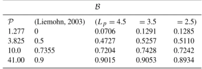
Table A1.Relation between pressure and disturbance ratios.
B
P (Liemohn, 2003) (Lp=4.5 =3.5 =2.5)
1.277 0 0.0706 0.1291 0.1285
3.825 0.5 0.4727 0.5257 0.5110
10.0 0.7355 0.7204 0.7428 0.7242
41.00 0.9 0.9015 0.9053 0.8934
(the additional integrations over angles, common to both terms, are not shown). From Eqs. (A1), (A2), (A3), and (A4), the disturbance ratio can be calculated in closed form:
B=1−[(x+1) /3I δ] (A5)
I ≡ex+1hp2+2pδ+3δ2i
−hx1+2δ+2δ2+21+3δ+4δ2i whereδ≡1L/Lb p≡Lp/Lb=1−xδ .
In Table A1, the pressure and disturbance ratios given by Eqs. (A3) and (A5), with Lb=6.5 held fixed and Lp
var-ied, are compared with the corresponding values from the model of Liemohn (2003). The first column contains the as-sumedP values and the second column theBvalues from
Table 1 (isotropic case only) of Liemohn (2003). The re-maining columns contain the B values calculated here for
each assumedP with variousLp, solving Eq. (A3)
numeri-cally forx as a function ofP, determining1Lfromx, and
inserting into Eq. (A5). It is evident that the agreement is suf-ficiently good (particularly in view of the different assump-tions concerning the loss cone) to confirm the reinterpreta-tion proposed here: removing the supposed truncareinterpreta-tion cur-rent term is nothing else than merely including the surface term that necessarily is present if the volume is bounded and the pressure at the boundary is not zero.
Alternatively, if use of a bounded volume is viewed as a way of isolating the contribution from that volume to the total disturbance fieldb(0), the expressions given by the Dessler-Parker-Sckopke theorem and by the Biot-Savart integral need not give the same result. The equivalence of the two expres-sions holds only for the complete integrals and not for the integrands (this is particularly apparent from the proof of the equivalence in Vasyli¯unas, 2001); when only partial contri-butions are evaluated, the so-called truncation current term is the difference.
Acknowledgements. I am grateful to M. W. Liemohn for discussion of the models in Liemohn (2003), to A. J. Dessler for calling my attention to the work of Piddington (1960), to M. G. Kivelson and to the referees for useful comments.
References
Alexeev, I. I., Belenkaya, E. S., Kalegaev, V. V., Feldstein, Y. I., and Grafe, A.: Magnetic storms and magnetotail currents, J. Geo-phys. Res., 101, 7737–7747, 1996.
Arykov, A. A. and Maltsev, Yu. P.: Direct-driven mechanism for geomagnetic storms, Geophys. Res. Lett., 23, 1689–1692, 1996. Baker, J. and Hurley, J.: A self-consistent study of the Earth’s
radi-ation belts, J. Geophys. Res., 72, 4351–4355, 1967.
Burton, R. K., McPherron, R. L., and Russell, C. T.: An empirical relationship between interplanetary conditions andDst, J. Geo-phys. Res., 80, 4204–4214, 1975.
Carovillano, R. L. and Maguire, J. J.: Magnetic energy relationships in the magnetosphere, in: Physics of the Magnetosphere, edited by: Carovillano, R. L., McClay, J. F., and Radoski, H. R., D. Reidel Publishing Co., Dordrecht–Holland, 270–300, 1968. Carovillano, R. L. and Siscoe, G. L.: Energy and momentum
theo-rems in magnetospheric dynamics, Rev. Geophys. Space Phys., 11, 289–353, 1973.
Chandrasekhar, S.: Hydrodynamic and Hydromagnetic Stability, Oxford University Press, 1961.
Crooker, N. U. and Siscoe, G. L.: Model geomagnetic disturbance from asymmetric ring current particles, J. Geophys. Res., 79, 589–594, 1974.
Crooker, N. U. and Siscoe, G. L.: Birkeland currents as the cause of the low-latitude asymmetric disturbance field, J. Geophys. Res., 86, 11 201–11 210, 1981.
Dessler, A. J. and Parker, E. N.: Hydromagnetic theory of geomag-netic storms, J. Geophys. Res., 24, 2239–2252, 1959.
Dungey, J. W.: The length of the magnetospheric tail, J. Geophys. Res., 70, 1753, 1965.
Feldstein, Y. I., Dremukhina, L. A., Levitin, A. E., Mall, U., Alex-eev, I. I., and Kalegaev, V. V.: Energetics of the magnetosphere during the magnetic storm, J. Atmos. Solar-Terr. Phys., 65, 429– 446, 2003.
Friedrich, E., Rostoker, G., Connors, M. G., and McPherron, R. L.: Influence of the substorm current wedge on theDst index, J. Geophys. Res., 104, 4567–4575, 1999.
Jordanova, V. K., Farrugia, C. J., Janoo, L., Quinn, J. M., Torbert, R. B., Ogilvie, K. W., Lepping, R. P., Steinberg, J. T., McComas, D. J., and Belian, R. D.: October 1995 magnetic cloud and ac-companying storm activity: Ring current evolution, J. Geophys. Res., 103, 79–92, 1998.
Jordanova, V. K., Kistler, L. M., Thomsen, M. F., and Muikis, C. G.: Effects of plasma sheet variability on the fast ini-tial ring current decay, Geophys. Res. Lett., 30(6), 1311, doi:10.1029/2002GL016576, 2003.
Koskinen, H. E. J. and Tanskanen, E.: Magnetospheric energy bud-get and the epsilon parameter, J. Geophys. Res., 107 (A11), 1415, doi:10.1029/2002JA009283, 2002.
Liemohn, M. W.: Yet another caveat to using the Dessler-Parker-Sckopke relation, J. Geophys. Res., 108(A6), 1251, doi:10.1029/2003JA009839, 2003.
Liemohn, M. W., Kozyra, J. U., Thomsen, M. F., Roeder, J. L., Lu, G., Borovsky, J. E. and Cayton, T. E.: Dominant role of the asymmetric ring current in producing the stormtimeDst*, J. Geophys. Res., 106, 10 883–10 904, 2001.
Liemohn, M. W., Kozyra, J. U., Clauer, C. R., Khazanov, G. V., and Thomsen, M. F.: Adiabatic energization in the ring current and its relation to other source and loss terms, J. Geophys. Res.,
107(4), 1045, doi:10.1029/2001JA000243, 2002.
Maguire, J. J., and Carovillano, R. L.: The kinetic energy and mag-netic disturbance of a trapped particle distribution, Trans. AGU, 48, 155, 1967.
Maltsev, Y. P. and Ostapenko, A. A.: Comment on “Evaluation of the tail current contribution toDst” by N. E. Turner et al., J. Geo-phys. Res., 107, A1, 1010, doi:10.1029/2001JA900098, 2002. Mayaud, P. N.: Derivation, Meaning, and Use of Geomagnetic
In-dices, Geophys. Monogr. Ser., vol. 22, AGU, Washington, D.C., 1980.
McPherron, R. L. and O’Brien, T. P.: Predicting geomagnetic activ-ity: TheDstindex, in: Space Weather, Geophys. Monogr. Ser., vol. 125, edited by: Song, P., Singer, H. J., and Siscoe, G. L., AGU, Washington, D.C., 339–345, 2001.
Munsani, V.: Determination of the effects of substorms on the storm-time ring current using neural networks, J. Geophys. Res., 105, 27 833–27 840, 2000.
O’Brien, T. P. and McPherron, R. L.: An empirical phase space analysis of ring current dynamics: Solar wind control of injection and decay, J. Geophys. Res., 105, 7707–7719, 2000.
O’Brien, T. P. and McPherron, R. L.: Seasonal and diurnal vari-ation of Dst dynamics, J. Geophys. Res., 107(A11), 1341, doi:10.1029/2002JA009435, 2002.
Ohtani, S., Nos´e, M., Rostoker, G., Singer, H., Lui, A. T. Y., and Nakamura, M.: Storm-substorm relationship: Contribution of the tail current toDst, J. Geophys. Res., 106, 21 199–21 2090, 2001. Olbert, S., Siscoe, G. L., and Vasyli¯unas, V. M.: A simple derivation of the Dessler–Parker–Sckopke relation, J. Geophys. Res., 73, 1115–1116, 1968.
Ostapenko, A. A. and Maltsev, Yu. P.: Three-dimensional magne-tospheric response to variations in the solar wind dynamic pres-sure, Geophys. Res. Lett., 25, 261–263, 1998.
Ostapenko, A. A. and Maltsev, Y. P.: Storm time variation in the magnetospheric magnetic field, J. Geophys. Res., 105, 311–316, 2000.
Parker, E. N.: Interaction of the solar wind with the geomagnetic field, Phys. Fluids, 1, 171–187, 1958.
Parker, E. N.: Nonsymmetric inflation of a magnetic dipole, J. Geo-phys. Res., 71, 4485–4494, 1966.
Piddington, J. H.: Geomagnetic storm theory, J. Geophys. Res., 65, 93–106, 1960.
Rossi, B. and Olbert, S.: Introduction to the Physics of Space, McGraw–Hill, New York, 1970.
Sckopke, N.: A general relation between the energy of trapped par-ticles and the disturbance field near the Earth, J. Geophys. Res., 71, 3125–3130, 1966.
Siscoe, G. L.: The virial theorem applied to magnetospheric dy-namics, J. Geophys. Res., 75, 5340–5350, 1970.
Siscoe, G. L. and Crooker, N. U.: On the partial ring current contri-bution toDst, J. Geophys. Res., 79, 1110–1112, 1974.
Siscoe, G. L. and Petschek, H. E.: On storm weakening during sub-storm expansion phase, Ann. Geophys., 15, 211–216, 1997. Siscoe, G. L., McPherron, R. L., Liemohn, M. W., Ridley, A. J., and
Lu, G.: Reconciling prediction algorithms forDst, J. Geophys. Res., 110, A02215, doi:10.1029/2004JA010465, 2005a. Siscoe, G. L., McPherron, R. L., and Jordanova, V. K.: Diminished
Song, P., Vasyli¯unas, V. M., and Ma, L.: A three-fluid model of so-lar wind-magnetosphere-ionosphere-thermosphere coupling, in: Multiscale Coupling of Sun-Earth Processes, edited by: Lui, A. T. Y., Kamide, Y., and Consolini, G., Elsevier, Amsterdam, The Netherlands, 447–456, 2005.
Spreiter, J. R., Alksne, A. Y., and Summers, A. L.: External aerody-namics of the magnetosphere, in: Physics of the Magnetosphere, edited by: Carovillano, R. L., McClay, J. F., and Radoski, H. R., D. Reidel Publishing Co., Dordrecht–Holland, 301–375, 1968. Turner, N. E., Baker, D. N., Pulkkinen, T. I., and McPherron, R. L.:
Evaluation of the tail current contribution toDst, J. Geophys. Res., 105, 5431–5439, 2000.
Turner, N. E., Pulkkinen, T. I., Baker, D. N., and McPher-ron, R. L.: Reply, J. Geophys. Res., 107, A1, 1011, doi:10.1029/2001JA900099, 2002.
Vasyli¯unas, V. M.: Comment on “Simulation study on fundamen-tal properties of the storm-time ring current” by Y. Ebihara and M. Ejiri, J. Geophys. Res., 106, 6321–6322, 2001.
Vasyli¯unas, V. M.: Reinterpreting the Burton-McPherron-Russell equation for predicting Dst, J. Geophys. Res., in press, doi:10.1029/2005JA011440, 2006.
Vasyli¯unas, V. M. and Song, P.: Meaning of iono-spheric Joule heating, J. Geophys. Res., 110, A02301, doi:10.1029/2004JA010615, 2005.