ACPD
14, 29019–29055, 2014Profiles of second- to third-order moments
of turbulent temperature fluctuations
A. Behrendt et al.
Title Page
Abstract Introduction
Conclusions References
Tables Figures
◭ ◮
◭ ◮
Back Close
Full Screen / Esc
Printer-friendly Version
Interactive Discussion
Discussion
P
a
per
|
Discussion
P
a
per
|
Discussion
P
a
per
|
Discussion
P
a
per
|
Atmos. Chem. Phys. Discuss., 14, 29019–29055, 2014 www.atmos-chem-phys-discuss.net/14/29019/2014/ doi:10.5194/acpd-14-29019-2014
© Author(s) 2014. CC Attribution 3.0 License.
This discussion paper is/has been under review for the journal Atmospheric Chemistry and Physics (ACP). Please refer to the corresponding final paper in ACP if available.
Profiles of second- to third-order
moments of turbulent temperature
fluctuations in the convective boundary
layer: first measurements with Rotational
Raman Lidar
A. Behrendt1, V. Wulfmeyer1, E. Hammann1, S. K. Muppa1, and S. Pal2
1
University of Hohenheim, Institute of Physics and Meteorology, 70599 Stuttgart, Germany
2
University of Virginia, Department of Environmental Sciences, Charlottesville, VA 22904, USA
Received: 9 July 2014 – Accepted: 24 October 2014 – Published: 21 November 2014
Correspondence to: A. Behrendt ([email protected])
ACPD
14, 29019–29055, 2014Profiles of second- to third-order moments
of turbulent temperature fluctuations
A. Behrendt et al.
Title Page
Abstract Introduction
Conclusions References
Tables Figures
◭ ◮
◭ ◮
Back Close
Full Screen / Esc
Printer-friendly Version
Interactive Discussion
Discussion
P
a
per
|
Discussion
P
a
per
|
Discussion
P
a
per
|
Discussion
P
a
per
|
Abstract
The rotational Raman lidar of the University of Hohenheim (UHOH) measures atmo-spheric temperature profiles during daytime with high resolution (10 s, 109 m). The data contain low noise errors even in daytime due to the use of strong UV laser light (355 nm, 10 W, 50 Hz) and a very efficient interference-filter-based polychromator. In this paper,
5
we present the first profiling of the second- to forth-order moments of turbulent tem-perature fluctuations as well as of skewness and kurtosis in the convective boundary layer (CBL) including the interfacial layer (IL). The results demonstrate that the UHOH RRL resolves the vertical structure of these moments. The data set which is used for this case study was collected in western Germany (50◦53′50.56′′N, 6◦27′50.39′′E,
10
110 m a.s.l.) within one hour around local noon on 24 April 2013 during the
Inten-sive Observations Period (IOP) 6 of the HD(CP)2Observational Prototype Experiment
(HOPE), which is embedded in the German project HD(CP)2 (High-Definition Clouds
and Precipitation for advancing Climate Prediction). First, we investigated profiles of the noise variance and compared it with estimates of the statistical temperature
measure-15
ment uncertainty∆T based on Poisson statistics. The agreement confirms that photon
count numbers obtained from extrapolated analog signal intensities provide a lower es-timate of the statistical errors. The total statistical uncertainty of a 20 min temperature measurement is lower than 0.1 K up to 1050 m a.g.l. at noontime; even for single 10 s temperature profiles, it is smaller than 1 K up to 1000 m a.g.l.. Then we confirmed by
20
autocovariance and spectral analyses of the atmospheric temperature fluctuations that a temporal resolution of 10 s was sufficient to resolve the turbulence down to the inertial subrange. This is also indicated by the profile of the integral scale of the temperature fluctuations, which was in the range of 40 to 120 s in the CBL. Analyzing then profiles of the second-, third-, and forth-order moments, we found the largest values of all
mo-25
ments in the IL around the mean top of the CBL which was located at 1230 m a.g.l..
The maximum of the variance profile in the IL was 0.40 K2 with 0.06 and 0.08 K2 for
sig-ACPD
14, 29019–29055, 2014Profiles of second- to third-order moments
of turbulent temperature fluctuations
A. Behrendt et al.
Title Page
Abstract Introduction
Conclusions References
Tables Figures
◭ ◮
◭ ◮
Back Close
Full Screen / Esc
Printer-friendly Version
Interactive Discussion
Discussion
P
a
per
|
Discussion
P
a
per
|
Discussion
P
a
per
|
Discussion
P
a
per
|
nificantly different from zero inside the CBL but showed a negative peak in the IL with
a minimum of −0.72 K3 and values of 0.06 and 0.14 K3 for the sampling and noise
errors, respectively. The forth-order moment and kurtosis values throughout the CBL were quasi-normal.
1 Introduction 5
Temperature fluctuations and their vertical organization inherently govern the energy budget in the convective planetary boundary layer (CBL) by determining the vertical heat flux and modifying the interaction of vertical mean temperature gradient and tur-bulent transport (Wyngaard et al., 1971). Thus, the measurement of turtur-bulent temper-ature fluctuations and the characterizations of their statistics is essential for solving the
10
turbulent energy budget closure (Stull, 1988). In-situ measurements (near the ground, on towers, or on airborne platforms) sample certain regions of the CBL within certain periods and have been used since a long time for turbulence studies. But to the best our knowledge, there are no previous observations based on a remote sensing technique suitable for this important task, i.e., resolving temperature fluctuations in high
resolu-15
tion and covering simultaneously the CBL up to the interfacial layer (IL). In this work, we demonstrate that rotational Raman lidar (RRL) (Cooney, 1972; Behrendt, 2005) can fill this gap.
By simultaneous measurements of turbulence at the land surface and in the IL, the flux divergence and other key scaling variables for sensible and latent heat entrainment
20
fluxes can be determined, which is essential for the evolution of temperature and hu-midity in the CBL and for verifying turbulence parameterizations in mesoscale models (Sorbjan, 1996, 2001, 2005).
Traditionally, studies of atmospheric temperature turbulence in the CBL were per-formed with in-situ instrumentation operated on tethered balloons, helicopters, and
air-25
instan-ACPD
14, 29019–29055, 2014Profiles of second- to third-order moments
of turbulent temperature fluctuations
A. Behrendt et al.
Title Page
Abstract Introduction
Conclusions References
Tables Figures
◭ ◮
◭ ◮
Back Close
Full Screen / Esc
Printer-friendly Version
Interactive Discussion
Discussion
P
a
per
|
Discussion
P
a
per
|
Discussion
P
a
per
|
Discussion
P
a
per
|
taneous profiles of turbulent fluctuations with in-situ sensor and it is difficult to identify the exact location and characteristics of the IL.
This calls for new remote sensing technologies. These instruments can be oper-ated on different platforms and can provide excellent long-term statistics, if applied from ground-based platforms. Passive remote sensing techniques, however, show
dif-5
ficulties in achieving such coverage because of their inherent limitation in both range and time resolution as well as time dependent errors in the retrievals. E.g., Kadygrov et al. (2011) published a study on temperature turbulence based on passive remote sensing techniques. The authors used a scanning microwave temperature profiler to investigate boundary layer thermal turbulence and compared the results with the
ex-10
pected−5/3-power law of Kolmogorov (1991), however, only within the lowest 200 m
layer.
In recent years, new insights in CBL turbulence were provided by studies based on active remote sensing with different types of lidar systems. Elastic backscatter lidar (Pal et al., 2010, 2013), ozone differential absorption lidar (ozone DIAL) (Senffet al.,
15
1996), Doppler lidar (e.g., Wulfmeyer and Janjic, 2005; Lenschow et al., 2010), water vapor differential absorption lidar (WV DIAL) (e.g., Senff et al., 1994; Kiemle et al., 1997; Wulfmeyer, 1999a, b; Muppa et al., 2014), and water vapor Raman lidar (e.g., Wulfmeyer et al., 2010; Turner et al., 2014a, b) have been employed or a combina-tion of these techniques (e.g., Giez et al., 1996; Kiemle et al., 2007, 2011; Behrendt
20
et al., 2011a; Kalthoffet al., 2013). However, so far, turbulence profiling of the key CBL variable temperature was missing.
In general, daytime measurements are more challenging than nighttime measure-ments for lidar because of the higher solar background which increases the signal noise and even prohibits measurements for most Raman lidar instruments. In order to
25
ACPD
14, 29019–29055, 2014Profiles of second- to third-order moments
of turbulent temperature fluctuations
A. Behrendt et al.
Title Page
Abstract Introduction
Conclusions References
Tables Figures
◭ ◮
◭ ◮
Back Close
Full Screen / Esc
Printer-friendly Version
Interactive Discussion
Discussion
P
a
per
|
Discussion
P
a
per
|
Discussion
P
a
per
|
Discussion
P
a
per
|
Valdebenito et al., 2011), on the initiation of convection (Groenemeijer et al., 2009; Corsmeier et al., 2011), and on atmospheric stability indices (Behrendt et al., 2011; Corsmeier et al., 2011). Here, we are applying the formalism introduced by Lenschow et al. (2000) for the first time to the data of an RRL to study the extension of the variable set of lidar turbulence studies within the CBL to temperature.
5
The measurements discussed here were carried out at local noon on 24 April 2013
during the Intensive Observations Period (IOP) 6 of the HD(CP)2 Observational
Pro-totype Experiment (HOPE) which is embedded in the project High-Definition Clouds
and Precipitation for advancing Climate Prediction (HD(CP)2) of the German
Re-search Ministry. The UHOH RRL was positioned during this study at 50◦53′50.56′′N,
10
6◦27′50.39′′E, 110 m a.s.l. near the village of Hambach in western Germany where it
performed measurements between 1 April and 31 May 2013.
This paper is organized as follows. In Sect. 2, the setup of the UHOH RRL is de-scribed briefly; more details can be found in (Hammann et al., 2014). The meteoro-logical background and turbulence measurements are presented in Sect. 3. Finally,
15
conclusions are drawn in Sect. 4.
2 Setup of the UHOH RRL
The RRL technique is based on the fact that different portions of the pure rotational
backscatter spectrum show different temperature dependence. By extracting signals
our of these two portions and forming the signal ratio, one obtains a profile which, after
20
calibration, yields a temperature profile of the atmosphere (see, e.g., Behrendt, 2005 for details).
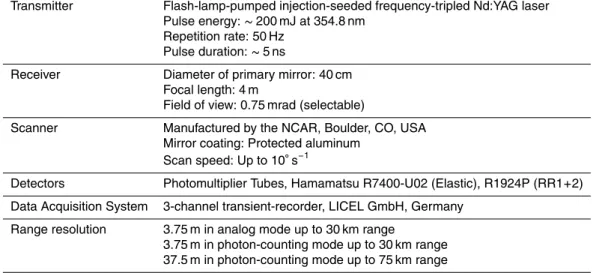
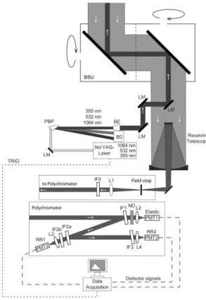
A scheme of the UHOH RRL during HOPE is shown in Fig. 1. Key system pa-rameters are summarized in Table 1. As laser source, an injection-seeded frequency-tripled Nd:YAG laser (354.8 nm, 50 Hz, 10 W), model GCR 290-50 of Newport
Spectra-25
ACPD
14, 29019–29055, 2014Profiles of second- to third-order moments
of turbulent temperature fluctuations
A. Behrendt et al.
Title Page
Abstract Introduction
Conclusions References
Tables Figures
◭ ◮
◭ ◮
Back Close
Full Screen / Esc
Printer-friendly Version
Interactive Discussion
Discussion
P
a
per
|
Discussion
P
a
per
|
Discussion
P
a
per
|
Discussion
P
a
per
|
prism (PBP) so that only the UV radiation is sent to the atmosphere. This improves eye-safety significantly compared to systems which use harmonic beam-splitters because definitely no potentially hazardous green laser light is present in the outgoing laser beam. But the main reason for using UV laser radiation for the transmitter of the UHOH RRL is that the backscatter cross section is proportional to the inverse wavelength to
5
the forth power. This yields significantly stronger signals and thus lower statistical un-certainties of the measurements in the lower troposphere (see also Di Girolamo et al., 2004; Behrendt, 2005; Di Girolamo et al., 2006) when using the third harmonic instead of the second harmonic of Nd:YAG laser radiation. Behind the PBP, the laser beam
is expanded 6.5-fold in order to reduce the beam divergence to<0.2 mrad. The laser
10
beam is then guided by three mirrors parallel to the optical axis of the receiving tele-scope (coaxial design) and reflected up into the atmosphere by two scanner mirrors. The same two mirrors reflect the atmospheric backscatter signals down to the receiv-ing telescope which has a primary mirror diameter of 40 cm. The scanner allows for full hemispherical scans with a scan speed of up to 10◦s−1. In the present case study, the
15
scanner was pointing constantly in vertical direction. In the focus of the telescope, an iris defines the field of view. For the data shown here, we selected an iris diameter of 3 mm yielding a telescope field of view of 0.75 mrad. The light is collimated behind the iris with a convex lens and enters a polychromator which contained three channels dur-ing the discussed measurements: one channel for collectdur-ing atmospheric backscatter
20
signals around the laser wavelength (elastic channel) and two channels for two signals
from different portions of the pure rotational Raman backscatter spectrum. During the
HOPE campaign, the polychromator was later extended with a water vapor Raman channel; the beamsplitter for this channel was already installed during the measure-ments discussed here. Within the polychromator, narrow-band multi-cavity interference
25
pass-ACPD
14, 29019–29055, 2014Profiles of second- to third-order moments
of turbulent temperature fluctuations
A. Behrendt et al.
Title Page
Abstract Introduction
Conclusions References
Tables Figures
◭ ◮
◭ ◮
Back Close
Full Screen / Esc
Printer-friendly Version
Interactive Discussion
Discussion
P
a
per
|
Discussion
P
a
per
|
Discussion
P
a
per
|
Discussion
P
a
per
|
bands were optimized within detailed performance simulations for measurements in the CBL in daytime (Behrendt, 2005; Radlach et al., 2008; Hammann et al., 2014). The new daytime/nighttime switch for the second rotational Raman channels (Hammann et al., 2014) was set to daytime.
3 Turbulence case study 5
3.1 Data set
The synoptic condition on 24 April 2013 was characterized by a large high-pressure system over central Europe. Because no clouds were forecasted for the HOPE region, this day was announced as Intensive Observation Period (IOP) 6 with the goal to study CBL development under clear-sky conditions. Indeed, undisturbed solar irradiance
re-10
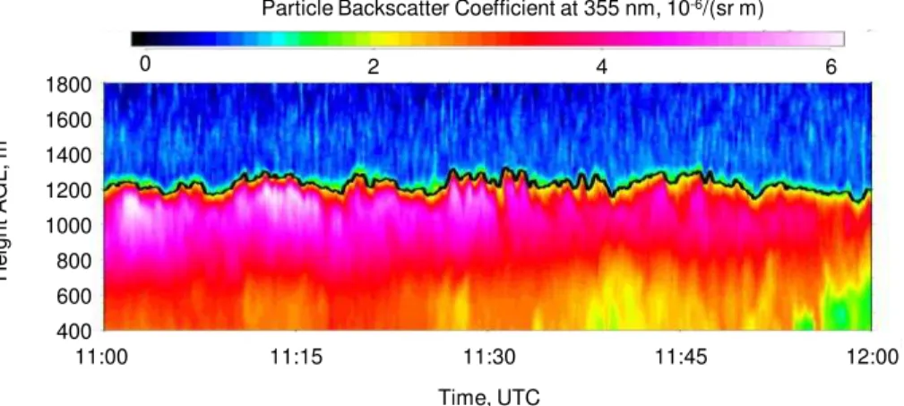
sulted in the development of a CBL which was not affected by clouds. The time-height
plot of the particle backscatter coefficientβpar (Fig. 2) between 11:00 and 12:00 UTC
shows the CBL around local noon (11:33 UTC with a maximum solar elevation of 54◦
on this day).βpar was measured with the rotational Raman lidar technique by use of
a temperature-independent reference signal. Data below 400 m were affected by
in-15
complete geometrical overlap of the outgoing laser beam and the receiving telescope and have been excluded from this study.
The instantaneous CBL height was determined with the Haar wavelet technique which detects the strongest gradient of the aerosol backscatter signal as tracer (Pal et al., 2010, 2012; Behrendt et al., 2011a) (Fig. 2). The mean of the instantaneous
20
CBL heightszi in the observation period was 1230 m a.g.l. This value is used in the
following for the normalized height scale z/zi. The standard deviation of the
instan-taneous CBL heights was 33 m; the absolute minimum and maximum were 1125 and 1323 m a.g.l., i.e., the instantaneous CBL heights were within 200 m.
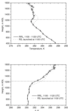
The UHOH RRL temperature profile of 11:00–11:20 UTC is shown in Fig. 3 together
25
ACPD
14, 29019–29055, 2014Profiles of second- to third-order moments
of turbulent temperature fluctuations
A. Behrendt et al.
Title Page
Abstract Introduction
Conclusions References
Tables Figures
◭ ◮
◭ ◮
Back Close
Full Screen / Esc
Printer-friendly Version
Interactive Discussion
Discussion
P
a
per
|
Discussion
P
a
per
|
Discussion
P
a
per
|
Discussion
P
a
per
|
Calibration of the RRL temperature data used in this study was made with these ra-diosonde data in the CBL between 400 and 1000 m a.g.l.; the RRL data above result from extrapolation of the calibration function. For the calibration, we used a 20 min
av-erage of the RRL data in order to reduce sampling effects between the two data sets.
For the statistical analysis of the turbulent temperature fluctuations, we used then this
5
calibration for the one-hour RRL data set between 11:00 and 12:00 UTC. This 1 h pe-riod seems here as a good compromise to us: for much longer pepe-riods, the CBL cannot be considered as being quasi-stationary anymore while shorter periods would reduce the number of sampled thermals and thus increase the sampling errors.
The temperature profiles of RRL and radiosonde shown in Fig. 3 agree within
frac-10
tions of a kelvin in the CBL. Larger differences occur in the IL due to the different sampling methods: the mean lidar profile shows an average over 20 min while the radiosonde data sample an instantaneous profile along the sonde’s path which was determined by the drift of the sonde with the horizontal wind. In this case, the sonde needed about 5 min to reach the top of the boundary layer and was drifted by about
15
1.6 km away from a vertical column above the site. Depending on the part of the ther-mal eddies in the CBL and the IL that are sampled, the radiosonde data represent thus different CBL features and are not representative for a mean profile (Weckwerth et al., 1996) which is a crucial point to be considered when using radiosonde data for scaling of turbulent properties in the CBL. Consequently, the lidar temperature data are more
20
representative for a certain site.
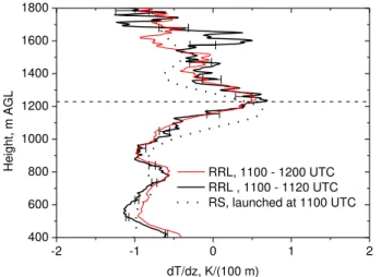
Inside the CBL, the potential temperature (derived from the RRL temperature data with the radiosonde pressure profile) is nearly constant indicating a well-mixed CBL (Fig. 3, lower panel).zi lies approximately in the middle of the temperature inversion in the IL (Fig. 3). Figure 4 shows the temperature gradients of the radiosonde and the
25
ACPD
14, 29019–29055, 2014Profiles of second- to third-order moments
of turbulent temperature fluctuations
A. Behrendt et al.
Title Page
Abstract Introduction
Conclusions References
Tables Figures
◭ ◮
◭ ◮
Back Close
Full Screen / Esc
Printer-friendly Version
Interactive Discussion
Discussion
P
a
per
|
Discussion
P
a
per
|
Discussion
P
a
per
|
Discussion
P
a
per
|
agrees with zi for both RRL profiles as determined with the Haar wavelet technique
while the height of the maximum gradient is about 60 m lower. As discussed above, the radiosonde data are not representative for a mean profile.
3.2 Turbulent temperature fluctuations
For CBL turbulence analyses, the instantaneous value of temperatureT(z) at heightz
5
is separated in a slowly varying or even constant componentT(z) derived from applying a linear fit to the data typically over 30 to 60 min and the temperature fluctuationT′(z)
according to
T(z)=T(z)+T′(z). (1)
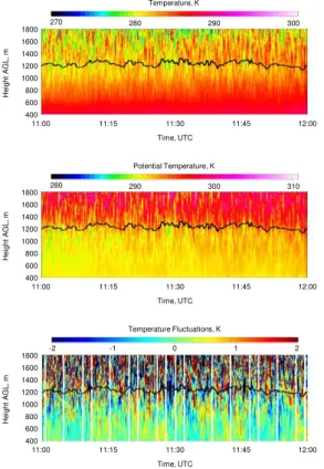
Figure 5 shows the time-height cross sections of temperature, potential temperature,
10
and detrended temperature fluctuationsT′(z) in the discussed period. For detrending,
a linear fit to the temperature time series was sufficient due to the quasi-stationary state of the CBL. One can see the positive and negative temperature fluctuations inside the CBL. In the IL, the fluctuations become larger than in heights below. Above the CBL in the free troposphere, one finds fewer structures in the temperature fluctuations and
15
mostly noise.
Lidar data contain significant stochastic instrumental noise, which has to be deter-mined and for which has to be corrected in order to obtain the atmospheric fluctuation of a variable of interest. In general, the signal-to-noise ratio can be improved by aver-aging the signal in time and/or range but this in turn would of course reduce the ability
20
to resolve turbulent structures. In principle, very high time resolution, i.e., the maximum allowed by the data acquisition system, is preferred in order to keep most frequencies of the turbulent fluctuations. But this is only possible as long as the derivation of tem-perature does not result in a non-linear increase of the noise errors; this noise regime should be avoided. A temporal resolution of 10 s turned out to be a good compromise
25
ACPD
14, 29019–29055, 2014Profiles of second- to third-order moments
of turbulent temperature fluctuations
A. Behrendt et al.
Title Page
Abstract Introduction
Conclusions References
Tables Figures
◭ ◮
◭ ◮
Back Close
Full Screen / Esc
Printer-friendly Version
Interactive Discussion
Discussion
P
a
per
|
Discussion
P
a
per
|
Discussion
P
a
per
|
Discussion
P
a
per
|
The variance of the atmosphere x′
a(z)
2
and the noise variance x′
n(z)
2
of a
vari-ablexare uncorrelated. Thus, we can write (Lenschow et al., 2000)
x′
m(z)
2 = x′
a(z)
2 + x′
n(z)
2
(2)
with x′
m(z)
2
or the measured total variance. Overbars denote here and in the fol-lowing mean temporal averages over the analysis period. The separation of the
atmo-5
spheric variance from the noise contribution to the total variance can be realized by
different techniques. Most straightforward is the autocovariance method, which makes
use of the fact that atmospheric fluctuations are correlated in time while instrumen-tal noise fluctuations are uncorrelated. Further details were introduced by Lenschow et al. (2000) so that only a brief overview is given here. By calculation of the
autoco-10
variance function (ACF) of a variable and extrapolating the function to zero lag with a power-law fit, one gets the variance of the atmosphere at the extrapolated value. As the ACF at zero lag is the total variance, the instrumental noise variance is the diff er-ence of the two. Alternatively, one may calculate the power spectrum of the fluctuations
and use Kolmogorows−5/3 law within the inertial subrange in order to determine the
15
noise level. We prefer the ACF method to the spectral analysis because it avoids adding
additional noise and systematic effects by conversion to the frequency space.
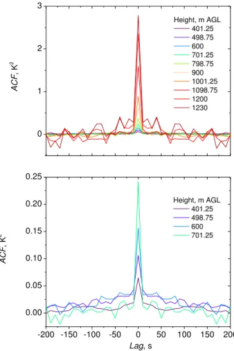
Figure 6 shows the ACF obtained from the measured temperature fluctuations for heights between 400 and 1230 m a.g.l., i.e., 0.3 to 1.0zi for lags from−200 to 200 s.
This interval was used for the extrapolation. The increase of the zero lag with height
20
ACPD
14, 29019–29055, 2014Profiles of second- to third-order moments
of turbulent temperature fluctuations
A. Behrendt et al.
Title Page
Abstract Introduction
Conclusions References
Tables Figures
◭ ◮
◭ ◮
Back Close
Full Screen / Esc
Printer-friendly Version
Interactive Discussion
Discussion
P
a
per
|
Discussion
P
a
per
|
Discussion
P
a
per
|
Discussion
P
a
per
|
3.3 Noise errors
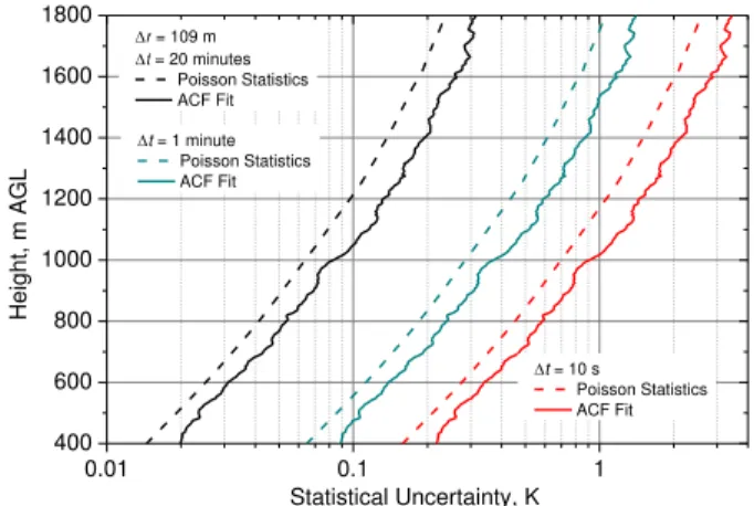
The resulting profiles of the total noise error of the temperature measurements
∆T(z)= r
T′
n(z)
2
(3)
are shown in Fig. 7 together with error profiles of the photon shot noise. Both profiles are similar but it should be noted that the autocovariance technique specifies the total
5
statistical error while Poisson statistics account only for the contribution of shot noise. Thus, the results of the Poisson statistics applied to the photon-count numbers provide a lower estimate for the total errors. The comparison confirms that the photon shot noise gives the main contribution and that other statistical error sources are compara-tively small.
10
For calculating the noise error from the signal intensities with Poisson statistics, the following approach was made: the lidar signals are detected simultaneously in analog and photon-counting mode. As the intensities of our rotational Raman signals are too strong, the photon-counting signals are affected by deadtime effects in lower heights than about 6 km in daytime. Correction of these deadtime effects (Behrendt et al., 2004)
15
is possible down to about 1.5 km. As this height limit is still too high for CBL studies, analog signals and not photon-counting signals have been used for the measurements of this study. In order to derive the statistical uncertainty of the measurements with Poisson statistics, the photon-counting signals of each 10 s profile were fitted to the analog signals in heights between about 1.5 and 3 km where both detection techniques
20
were providing reliable data after deadtime correction of the photon-counting data. By extrapolation, photon counting rates were then attributed to the analog signal intensi-ties in lower altitudes. These extrapolated count rates were consequently used. The background photon-counting numbers were derived from the photon-counting signals detected from high altitudes.
ACPD
14, 29019–29055, 2014Profiles of second- to third-order moments
of turbulent temperature fluctuations
A. Behrendt et al.
Title Page
Abstract Introduction
Conclusions References
Tables Figures
◭ ◮
◭ ◮
Back Close
Full Screen / Esc
Printer-friendly Version
Interactive Discussion
Discussion
P
a
per
|
Discussion
P
a
per
|
Discussion
P
a
per
|
Discussion
P
a
per
|
The statistical uncertainty of a signal with N photon counts according to Poisson
statistics is
∆N(z)= q
N(z). (4)
Error propagation then yields for the RRL temperature data (Behrendt et al., 2002)
∆T(z)= ∂T
∂Q
NRR2(z)
NRR1(z)
v u u u t
N∗
RR1(z)+
∆BRR1
2
(NRR1(z))
2 +
N∗
RR2(z)+
∆BRR2
2
(NRR2(z))
2 . (5)
5
with N∗
RR1(z) and NRR2∗ (z) for the photon counts in the two rotational Raman chan-nels before background correction. NRRi(z)=NRR∗ i(z)−BRRi with i =1, 2 are the
sig-nals which are corrected for background noise per range bin BRRi. The ratio of the
two number of photon countsNRR1 and NRR2 of lower and higher rotational quantum
number transition channels
10
Q=NRR2
NRR1 (6)
is the measurement parameter which yields the atmospheric temperature profile after
calibration of the system. Therefore,∂T/∂Qis provided by the temperature calibration
function.
Since the background is determined over many range bins, the statistical uncertainty
15
of the background can be neglected (Behrendt et al., 2004) so that one finally gets
∆T(z)= ∂T
∂Q
NRR2(z)
NRR1(z)
v u u
tNRR1(z)+BRR1
(NRR1(z))
2 +
NRR2(z)+BRR2
(NRR2(z))
2 . (7)
ACPD
14, 29019–29055, 2014Profiles of second- to third-order moments
of turbulent temperature fluctuations
A. Behrendt et al.
Title Page
Abstract Introduction
Conclusions References
Tables Figures
◭ ◮
◭ ◮
Back Close
Full Screen / Esc
Printer-friendly Version
Interactive Discussion
Discussion
P
a
per
|
Discussion
P
a
per
|
Discussion
P
a
per
|
Discussion
P
a
per
|
The background-corrected rotational Raman signals scale according to
NRRi(z)∝P∆t∆z ηtηrA. (8)
withi =1, 2, laser powerP, measurement time∆t, range resolution∆z, transmitter and receiver efficiency ηt andηr, and receiving telescope areaA. The background counts
in each signal range bin scale in a similar way but without being influenced by powerP
5
andηt, so that we get
BRRi(z)∝∆t∆z ηrA. (9)
One can see from Eqs. (7) to (9) that the statistical measurement uncertainty scales consequently with
∆T ∝p 1
∆t∆z ηrA
. (10)
10
It is noteworthy, that increases of the laser powerP and transmitter efficiency ηt are even more effective in reducing ∆T than increases of ∆t, ∆z, ηr, or A because the former improve only the backscatter signals and do not increase the background si-multaneously like the latter. The value of the improvement obtained from increases of
P orηt, however, depends on the intensity of the background and thus on height and
15
background-light conditions (see also Radlach et al., 2008; Hammann et al., 2014). The statistical uncertainties for the RRL temperature measurements at noontime shown in Fig. 7 were determined with 10 s temporal resolution and for range averaging of 109 m. The resulting error profiles for other temporal resolutions were then derived from the 10 s error profile by use of Eq. (10). The errors for other range resolutions can
20
be easily obtained from Eq. (10) in a similar way.
ACPD
14, 29019–29055, 2014Profiles of second- to third-order moments
of turbulent temperature fluctuations
A. Behrendt et al.
Title Page
Abstract Introduction
Conclusions References
Tables Figures
◭ ◮
◭ ◮
Back Close
Full Screen / Esc
Printer-friendly Version
Interactive Discussion
Discussion
P
a
per
|
Discussion
P
a
per
|
Discussion
P
a
per
|
Discussion
P
a
per
|
to about 1000 m a.g.l. With 1 min resolution,∆T is below 0.4 K up to 1000 m a.g.l. and
below 1 K up to 1530 m a.g.l. With 20 min averaging,∆T is below 0.1 and 0.3 K up to
1050 and 1770 m a.g.l., respectively.
3.4 Integral scale
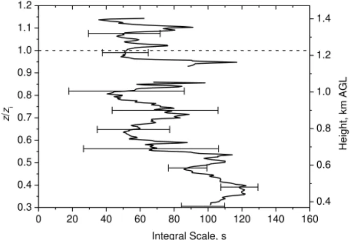
Figure 8 shows the profiling of the integral scale of the temperature fluctuations. It
5
was obtained with the 2/3-power-law fit for noise correction (Lenschow et al., 2000).
Data around 0.9zi, i.e., that height region where the variance is close to zero and thus
relative errors are very large show also relative noise errors larger than 100 % for the integral scale. Consequently, these data have been excluded from the analysis. The
integral scale shows values between (40±22) s and (122±12) s in the CBL. That the
10
integral scale is significantly larger than the temporal resolution of the UHOH RRL data of 10 s confirms that the resolution of our data is high enough to resolve the turbulent temperature fluctuations including the major part of the inertial subrange throughout the CBL. The integral time scale (which can be related to a length scale provided that the mean horizontal wind speed is known) is considered as a measure of the mean
15
size of the turbulent eddies involved in the boundary layer mixing processes.
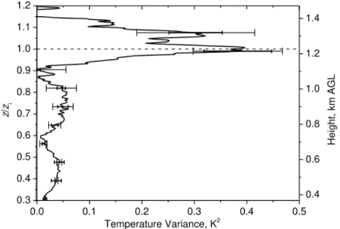
3.5 Temperature variance
What is to our best knowledge the first profile of the temperature variance of the
at-mosphere T′
a(z)
2
measured with a lidar system is shown in Fig. 9; the profile starts
at about 0.3 zi and covers the whole CBL. The variance profile was calculated with
20
the 2/3-power-law-fit method, as discussed above. Between 0.3 and 0.9 zi, the
vari-ance was much smaller than in the IL. Here the values are only up to 0.058 K2 (at
982 m=0.8zi with 0.010 and 0.024 K2for the sampling and noise error, respectively).
Taken the error bars into account, one finds that the apparent minimum at 0.9zi, is not statistically significant and the one at 0.6zi only weakly significant. What remains is
25
ACPD
14, 29019–29055, 2014Profiles of second- to third-order moments
of turbulent temperature fluctuations
A. Behrendt et al.
Title Page
Abstract Introduction
Conclusions References
Tables Figures
◭ ◮
◭ ◮
Back Close
Full Screen / Esc
Printer-friendly Version
Interactive Discussion
Discussion
P
a
per
|
Discussion
P
a
per
|
Discussion
P
a
per
|
Discussion
P
a
per
|
in the IL close tozi. This maximum of the variance profile was 0.40 K2with a sampling error of 0.06 and 0.08 K2 for the noise error (root-mean-square variability). Except at the surface, one expects that the temperature variance in a CBL is largest in the IL since the temporal variability is driven by entrainment caused by turbulent buoyancy-driven motions acting against the temperature inversion at the top of the CBL (e.g.,
5
Deardorff, 1974; André et al., 1978; Stull, 1988; Moeng and Wyngaard, 1989).
3.6 Third-order moment and skewness
The third-order moment (TOM) of a fluctuation is a measure of the asymmetry of the
distribution. The skewnessSis the TOM normalized by the variance to a dimensionless
parameter defined for temperature as
10
S(z)= (T′(z))
3
(T′(z))2
3/2
. (11)
The normal distribution (Gaussian curve) has zero TOM and S. Positive values for
TOM andS show a right-skewed distribution where the mode is smaller than the mean.
If the mode is larger than the mean, TOM andS become negative (left-skewed
distri-bution).
15
TOM and S profiles for the atmospheric temperature fluctuations of our case are
shown in Fig. 10. Up to about 0.9 zi, TOM was not different to zero (taking the 1-σ
statistical uncertainties into account). In the IL, i.e., between 0.9 and 1.1zi, a negative
peak is found with values down to−0.72 K3with 0.06 and 0.14 K3for the sampling and
noise errors, respectively. The skewness profile shows the same characteristics. Only
20
data around 0.9 zi had to be omitted from the analysis because the variance profile
becomes close to zero here and thus division by these values yielded too large relative errors. Atzi, we found a skewness of−3.2 with 0.9 and 1.3 for the sampling and noise
ACPD
14, 29019–29055, 2014Profiles of second- to third-order moments
of turbulent temperature fluctuations
A. Behrendt et al.
Title Page
Abstract Introduction
Conclusions References
Tables Figures
◭ ◮
◭ ◮
Back Close
Full Screen / Esc
Printer-friendly Version
Interactive Discussion
Discussion
P
a
per
|
Discussion
P
a
per
|
Discussion
P
a
per
|
Discussion
P
a
per
|
TOM and S profiles reveal interesting characteristics of the thermal plumes which
were present in the CBL in this case. We can conclude that the turbulent temperature fluctuations were not significantly skewed in the CBL; negative and positive fluctuations
were symmetric. The negative minimum in the IL shows a clear difference between
the IL and the CBL below. Between 0.9 and 1.1zi, negative and positive fluctuations
5
were not symmetric but fewer very cold fluctuations were balanced by many warm fluctuations with less difference to the mean.
Because turbulent mixing occurs in a region of positive vertical temperature gradient in the IL, the air present in the free troposphere is warmer than the air in the CBL below. Consequently, the negative peak indicates that the cold overshooting updrafts in the IL
10
were narrower in time than the downdrafts of warmer air.
Similar characteristics of the temperature TOM and skewness profiles in the CBL were discussed, e.g., by Mironov et al. (1999), Canuto et al. (2001), and Cheng et al. (2005) who compare experimental data (tank, wind tunnel, airborne in-situ), LES data, and analytical expressions.
15
3.7 Forth-order moment and kurtosis
Forth-order moment (FOM) is a measure of the steepness of the distribution. The kur-tosis is the FOM normalized by the variance to a dimensionless parameter according to
Kurtosis(z)= (T
′(z))4
(T′(z))2
2. (12)
20
ACPD
14, 29019–29055, 2014Profiles of second- to third-order moments
of turbulent temperature fluctuations
A. Behrendt et al.
Title Page
Abstract Introduction
Conclusions References
Tables Figures
◭ ◮
◭ ◮
Back Close
Full Screen / Esc
Printer-friendly Version
Interactive Discussion
Discussion
P
a
per
|
Discussion
P
a
per
|
Discussion
P
a
per
|
Discussion
P
a
per
|
Figure 11 shows FOM and kurtosis profiles of the measured temperature fluctuations of our case. For both FOM and kurtosis, the noise errors of the data are quite large; the importance of an error analysis becomes once more obvious. Throughout the CBL, no significant differences to the normal distribution are found. While the values for the FOM are close to zero in the CBL (<0.5 K4up to 0.9zi), they appear larger in the IL, but the
5
noise error does not allow for determining exact values, zero is still within the 1-σnoise error bars. Atzi, FOM was 2.7 K4with 0.2 and 3.7 K4for the sampling and noise errors, respectively. The kurtosis atzi was 20 with 7 and 28 for the sampling and noise errors,
respectively. We conclude that the distribution of atmospheric temperature fluctuations was not significantly different to a Gaussian distribution (quasi-normal) regarding its
10
forth-order moment and kurtosis in our case.
Even if the data is here too noisy to identify non-zero FOM or kurtosis in the IL, it is interesting to note that higher values of kurtosis in the IL would reflect a situation for which a large fraction of the temperature fluctuations occurring in this region would exist due to infrequent very large deviations in temperature; the related most vigorous
15
thermals would then be capable to yield quite extreme temperature fluctuations while mixing intensively in the IL with the air of the lower free troposphere. In contrast to this, the temperature fluctuations would be more moderate (Gaussian) in the CBL below.
4 Conclusions
We have shown that rotational Raman lidar offers a remote sensing technique for the
20
analysis of turbulent temperature fluctuations within the well-developed CBL during noontime – even though the background light conditions at noon are least favorable for measurements with rotational Raman lidar. We can state that the required high tempo-ral and spatial resolution combined with low-enough statistical noise of the measured data is reached by the UHOH RRL. The data can thus be evaluated during the all time
25
ACPD
14, 29019–29055, 2014Profiles of second- to third-order moments
of turbulent temperature fluctuations
A. Behrendt et al.
Title Page
Abstract Introduction
Conclusions References
Tables Figures
◭ ◮
◭ ◮
Back Close
Full Screen / Esc
Printer-friendly Version
Interactive Discussion
Discussion
P
a
per
|
Discussion
P
a
per
|
Discussion
P
a
per
|
Discussion
P
a
per
|
We have analyzed a case of the HOPE campaign. The data were collected be-tween 11:00 and 12:00 UTC on IOP 6, 24 April 2013, i.e., exactly around local noon (11:33 UTC). The UHOH RRL was located near the village of Hambach in western Germany (50◦53′50.56′′N, 6◦27′50.39′′E, 110 m a.s.l.).
A profile of the noise variance was used to estimate the statistical uncertainty∆T of
5
the temperature data with a 2/3 power law fit to the autocovariance function. A
com-parison with a ∆T profile derived with Poisson statistics demonstrated that the
sta-tistical error is mainly due to shot noise. The Haar wavelet technique was applied to
10 s profiles ofβpar and provided the mean CBL height over the observation period of
zi =1230 m a.g.l. This value is used for normalizing the height scale.
10
The results of this study give further information on turbulent temperature fluctuations and their statistics in the CBL and within the IL. The integral scale profile shows values
between (40±22) s and (122±12) s in the CBL. Thus, we can confirm that the
tempo-ral resolution of the RRL data of 10 s was sufficiently high for resolving the major part of turbulence down to the inertial subrange. The atmospheric variance profile showed
15
clearly the largest values close to zi. A maximum of the variance of the atmospheric
temperature fluctuations was found in the IL: 0.40 K2with a sampling and noise error of 0.06 and 0.08 K2, respectively. Subsequently, we also derived profiles of the third- and
forth-order moments. TOM and skewness were not significantly different to zero within
the CBL up to about 0.9zi. In the IL between 0.9 and 1.1zi, a negative minimum was
20
found with values down to−0.72 K3with 0.06 and 0.14 K3for the sampling and noise
errors, respectively. Skewness atzi was −3.2 and with 0.9 and 1.3 for the sampling
and noise errors, respectively. We conclude that the turbulent temperature fluctuations were not significantly skewed in the CBL. In contrast to this, the atmospheric temper-ature fluctuations in the IL were clearly skewed to the left (negative skewness). This
25
mo-ACPD
14, 29019–29055, 2014Profiles of second- to third-order moments
of turbulent temperature fluctuations
A. Behrendt et al.
Title Page
Abstract Introduction
Conclusions References
Tables Figures
◭ ◮
◭ ◮
Back Close
Full Screen / Esc
Printer-friendly Version
Interactive Discussion
Discussion
P
a
per
|
Discussion
P
a
per
|
Discussion
P
a
per
|
Discussion
P
a
per
|
ments but especially the FOM, the importance of an error analysis became once more obvious.
A quasi-normal FOM even when TOM is non-zero, agrees with the hypothesis of Millionshchikov (1941) which forms the basis for a large number of closure models (see Gryanik et al., 2005 for an overview). However, some recent theoretical studies,
5
measurement data, and LES data suggest that this hypothesis would not be valid for temperature in the CBL (see also see Gryanik et al., 2005 for an overview).
It is planned to extend the investigation of CBL characteristics in future studies by combining the UHOH RRL data with humidity and wind observations from water vapor DIAL (Muppa et al., 2014; Späth et al., 2014) and Doppler lidar. Furthermore, also the
10
scanning capability of the UHOH RRL will be used in future to collect data closer to the ground and even the surface layer (Behrendt et al., 2012) in order to investigate heterogeneities over different terrain.
The combination of different turbulent parameters measured by lidar – preferably, at the same atmospheric coordinates simultaneously – promises to provide further
un-15
derstanding on the important processes taking place in the CBL including the IL. For instance, till date, the key physical processes governing the IL and their relationships with other CBL properties remain unfortunately only poorly understood: they are over-simplified in empirical studies and poorly represented in the models. In consequence, more data should be evaluated to get the statistics of temperature turbulence under
20
a variety of atmospheric conditions. We believe that temperature turbulence profiling with RRL will contribute significantly to better understanding of boundary layer mete-orology in the future – not only in daytime but also at night so that the entire diurnal cycle is covered and the characteristics of temperature turbulence in different stability regimes can be observed.
ACPD
14, 29019–29055, 2014Profiles of second- to third-order moments
of turbulent temperature fluctuations
A. Behrendt et al.
Title Page
Abstract Introduction
Conclusions References
Tables Figures
◭ ◮
◭ ◮
Back Close
Full Screen / Esc
Printer-friendly Version
Interactive Discussion
Discussion
P
a
per
|
Discussion
P
a
per
|
Discussion
P
a
per
|
Discussion
P
a
per
|
References
André, J. C., De Moor, G., Lacarrère, P., Therry, G., and Du Vachat, R.: Modeling the 24-hour evolution of the mean and turbulent structures of the planetary boundary layer, J. Atmos. Sci., 35, 1861–1883, 1978.
Behrendt, A.: Temperature measurements with lidar, in: Lidar: Range-Resolved Optical Remote 5
Sensing of the Atmosphere, edited by: Weitkamp, C., Springer, New York, 273–305, 2005. Behrendt, A. and Reichardt, J.: Atmospheric temperature profiling in the presence of clouds
with a pure rotational Raman lidar by use of an interference-filter-based polychromator, Appl. Optics, 39, 1372–1378, 2000.
Behrendt, A., Nakamura, T., Onishi, M., Baumgart, R., and Tsuda, T.: Combined Raman lidar 10
for the measurement of atmospheric temperature, water vapor, particle extinction coefficient, and particle backscatter coefficient, Appl. Optics, 41, 7657–7666, 2002.
Behrendt, A., Nakamura, T., and Tsuda, T.: Combined temperature lidar for measurements in the troposphere, stratosphere, and mesosphere, Appl. Optics, 43, 2930–2939, 2004. Behrendt, A., Pal, S., Aoshima, F., Bender, M., Blyth, A., Corsmeier, U., Cuesta, J., Dick, G., 15
Dorninger, M., Flamant, C., Di Girolamo, P., Gorgas, T., Huang, Y., Kalthoff, N., Khodayar, S., Mannstein, H., Träumner, K., Wieser, A., and Wulfmeyer, V.: Observation of convection initi-ation processes with a suite of state-of-the-art research instruments during COPS IOP8b, Q. J. Roy. Meteor. Soc., 137, 81–100, doi:10.1002/qj.758, 2011a.
Behrendt, A., Pal, S., Wulfmeyer, V., Valdebenito B., Á. M., and Lammel, G.: A novel approach 20
for the char-acterisation of transport and optical properties of aerosol particles near sources, Part I: measurement of particle backscatter coefficient maps with a scanning UV lidar, Atmos. Environ., 45, 2795–2802, doi:10.1016/j.atmosenv.2011.02.061, 2011b.
Behrendt, A., Hammann, E., Späth, F., Riede, A., Metzendorf, S., and Wulfmeyer, V.: Revealing surface layer heterogeneities wit scanning water vapor DIAL and scanning rotational Raman 25
lidar, in: Reviewed and Revised Papers Presented at the 26th International Laser Radar Conference (ILRC 2012), 25–29 June 2012, Porto Heli, Greece, edited by: Papayannis, A., Balis, D., and Amiridis, V., paper S7P-17, 913–916, 2012.
Canuto, V. M., Chang, Y., and Howard, A.: New third-order moments for the convective bound-ary layer, J. Atmos. Sci., 58, 1169–1172, 2001.
30
ACPD
14, 29019–29055, 2014Profiles of second- to third-order moments
of turbulent temperature fluctuations
A. Behrendt et al.
Title Page
Abstract Introduction
Conclusions References
Tables Figures
◭ ◮
◭ ◮
Back Close
Full Screen / Esc
Printer-friendly Version
Interactive Discussion
Discussion
P
a
per
|
Discussion
P
a
per
|
Discussion
P
a
per
|
Discussion
P
a
per
|
Clarke, R. H., Dyer, A. J., Brook, R. R., Reid, D. G., and Troup, A. J.: The Wangara experi-ment: Boundary layer data. Tech. Paper No. 19, CSIRO, Division of Meteorological Physics, Aspendale, Australia, 362 pp., 1971.
Cooney, J.: Measurement of atmospheric temperature profiles by Raman backscatter, J. Appl. Meteorol., 11, 108–112, 1972.
5
Corsmeier, U., Kalthoff, N., Barthlott, Ch., Behrendt, A., Di Girolamo, P., Dorninger, M., Aoshima, F., Handwerker, J., Kottmeier, C., Mahlke, H., Mobbs, S., Vaughan, G., Wickert, J., and Wulfmeyer, V.: Driving processes for deep convection over complex terrain: a multi-scale analysis of observations from COPS-IOP 9c, Q. J. Roy. Meteor. Soc., 137, 137–155, doi:10.1002/qj.754, 2011.
10
Deardorff, J. W.: Three-dimensional numerical study of turbulence in an entraining mixed layer, Bound.-Lay. Meteorol., 7, 199–226, 1974.
Di Girolamo, P., Marchese, R., Whiteman, D. N., and Demoz, B.: Rotational Raman lidar measurements of atmospheric temperature in the UV, Geophys. Res. Lett., 31, L01106, doi:10.1029/2003GL018342, 2004.
15
Di Girolamo, P., Behrendt, A., and Wulfmeyer, V.: Spaceborne profiling of atmospheric tem-perature and particle extinction with pure rotational Raman lidar and of relative humidity in combination with differential absorption lidar: performance simulations, Appl. Optics, 45, 2474–2494, 2006.
Giez, A., Ehret, G., Schwiesow, R. L., Davis, K. J., and Lenschow, D. H.: Water vapor flux 20
measurements from ground-based vertically pointed water vapor differential absorption and Doppler lidars, J. Atmos. Ocean. Tech., 16, 237–250, 1999.
Groenemeijer, P., Barthlott, C., Behrendt, A., Corsmeier, U., Handwerker, J., Kohler, M., Kottmeier, C., Mahlke, H., Pal, S., Radlach, M., Trentmann, J., Wieser, A., and Wulfmeyer, V.: Multi-sensor measurements of a convective storm cluster over a low moun-25
tain range: adaptive observations during PRINCE, Mon. Weather Rev., 137, 585–602, doi:10.1175/2008MWR2562.1, 2009.
Gryanik, V. M., Hartmann, J., Raasch, S., and Schröter, M.: A refinement of the Millionshchikov Quasi-Normality Hypothesis for convective boundary layer turbulence, J. Atmos. Sci., 62, 2632–2638, 2005.
30
ACPD
14, 29019–29055, 2014Profiles of second- to third-order moments
of turbulent temperature fluctuations
A. Behrendt et al.
Title Page
Abstract Introduction
Conclusions References
Tables Figures
◭ ◮
◭ ◮
Back Close
Full Screen / Esc
Printer-friendly Version
Interactive Discussion
Discussion
P
a
per
|
Discussion
P
a
per
|
Discussion
P
a
per
|
Discussion
P
a
per
|
prototype experiment, Atmos. Chem. Phys. Discuss., 14, 28973–29018, doi:10.5194/acpd-14-28973-2014, 2014
Kadygrov, E. N., Shur, G. N., and Viazankin, A. S.: Investigation of atmospheric boundary layer temperature, turbulence, and wind parameters on the basis of passive microwave remote sensing, Radio Sci., 38, 8048, doi:10.1029/2002RS002647, 2003.
5
Kalthoff, N., Träumner, K., Adler, B., Späth, S., Behrendt, A., Wieser, A., Handwerker, J., Madonna, F., and Wulfmeyer, V.: Dry and moist convection in the boundary layer over the Black Forest – a combined analysis of in situ and remote sensing data, Meteorol. Z., 22, 445–461, doi:10.1127/0941-2948/2013/0417, 2013.
Kiemle, C., Ehret, G., Giez, A., Davis, K. J., Lenschow, D. H., and Oncley, S. P.: Estimation 10
of boundary layer humidity fluxes and statistics from airborne differential absorption lidar (DIAL), J. Geophys Res., 102, 29189–29203, 1997.
Kiemle, C., Brewer, W. A., Ehret, G., Hardesty, R. M., Fix, A., Senff, C., Wirth, M., Poberaj, G., and LeMone, M. A.: Latent heat flux profiles from collocated airborne water vapor and wind lidars during IHOP 2002, J. Atmos. Ocean. Tech., 24, 627–639, 2007.
15
Kiemle, C., Wirth, M., Fix, A., Rahm, S., Corsmeier, U., and Di Girolamo, P.: Latent heat fluxes over complex terrain from airborne water vapour and wind lidars, Q. J. Roy. Meteor. Soc., 137, 190–203, 2011.
Kolmogorov, A. N.: The Local Structure of Turbulence in Incompressible Viscous Fluid for Very Large Reynolds Numbers, Proc. R. Soc. Lond., A 434, 1890, 9–13, 20
doi:10.1098/rspa.1991.0075, 1991.
Lenschow, D. H., Wulfmeyer, V., and Senff, C.: Measuring second through fourth-order mo-ments in noisy data, J. Atmos. Ocean. Tech., 17, 1330–1347, 2000.
Lenschow, D. H., Lothon, M., Mayor, S. D., Sullivan, P. P., and Caunt., G.: A comparison of higher-order vertical velocity statistics in the convective boundary layer from lidar with in-situ 25
measurements and large-eddy simulations, Bound.-Lay. Meteorol., 143, 107–123, 2012. Martin, S., Bange, J., and Beyrich, F.: Meteorological profiling of the lower troposphere using
the research UAV “M2AV Carolo”, Atmos. Meas. Tech., 4, 705–716, doi:10.5194/amt-4-705-2011, 2011.
Millionshchikov, M. D.: On the Theory of Homogeneous Isotropic Turbulence, Dokl. Akad. Nauk 30
ACPD
14, 29019–29055, 2014Profiles of second- to third-order moments
of turbulent temperature fluctuations
A. Behrendt et al.
Title Page
Abstract Introduction
Conclusions References
Tables Figures
◭ ◮
◭ ◮
Back Close
Full Screen / Esc
Printer-friendly Version
Interactive Discussion
Discussion
P
a
per
|
Discussion
P
a
per
|
Discussion
P
a
per
|
Discussion
P
a
per
|
Mironov, D. V., Gryanik, M., Lykossov, V. N., and Zilitinkevich, S. S.: Comments on “A new second-order turbulence closure scheme for the planetary boundary layer”, J. Atmos. Sci., 56, 3478–3481, 1999.
Moeng, C.-H. and Wyngaard, J. C.: Evaluation of turbulent transport and dissipation closures in second-order modelling, J. Atmos. Sci., 46, 2311–2330, 1989.
5
Muppa, S. K., Behrendt, A., Späth, F., Wulfmeyer, V., Metzendorf, S., and Riede, A.: Turbulent humidity fluctuations in the convective boundary layer: case studies using DIAL measure-ments, Atmos. Chem. Phys. Discuss., in preparation, 2014.
Muschinski, A., Frehlich, R., Jensen, M., Hugo, R., Eaton, F., and Balsley, B.: Fine-scale mea-surements of turbulence in the lower troposphere: an intercomparison between a kite- and 10
balloon-borne, and a helicopter-borne measurement system, Bound.-Lay. Meteorol., 98, 219–250, 2001.
Pal, S., Behrendt, A., and Wulfmeyer, V.: Elastic-backscatter-lidar-based characterization of the convective boundary layer and investigation of related statistics, Ann. Geophys., 28, 825–847, doi:10.5194/angeo-28-825-2010, 2010.
15
Pal, S., Xueref-Remy, I., Ammoura, L., Chazette, P., Gibert, F., Royer, P., Dieudonné, E., Dupont, J. C., Haeffelin, M., Lac, C., Lopez, M., Morille, Y., and Ravetta, F.: Spatio-temporal variability of the atmospheric boundary layer depth over the Paris agglomeration: an assess-ment of the impact of the urban heat island intensity, Atmos. Environ., 63, 261–275, 2012. Pal, S., Haeffelin, M, and Batchvarova, E. Exploring a geophysical process-based attribution 20
technique for the determination of the atmospheric boundary layer depth using aerosol li-dar and near-surface meteorological measurements, J. Geophys. Res.-Atmos., 118, 1–19, doi:10.1002/jgrd.50710, 2013.
Radlach, M., Behrendt, A., and Wulfmeyer, V.: Scanning rotational Raman lidar at 355 nm for the measurement of tropospheric temperature fields, Atmos. Chem. Phys., 8, 159–169, 25
doi:10.5194/acp-8-159-2008, 2008.
Senff, C. J., Bösenberg, J., and Peters, G.: Measurement of water vapor flux profiles in the convective boundary layer with lidar and Radar-RASS, J. Atmos. Ocean. Tech., 11, 85–93, 1994.
Senff, C. J., Bösenberg, J., Peters, G., and Schaberl, T.: Remote sensing of turbulent ozone 30
ACPD
14, 29019–29055, 2014Profiles of second- to third-order moments
of turbulent temperature fluctuations
A. Behrendt et al.
Title Page
Abstract Introduction
Conclusions References
Tables Figures
◭ ◮
◭ ◮
Back Close
Full Screen / Esc
Printer-friendly Version
Interactive Discussion
Discussion
P
a
per
|
Discussion
P
a
per
|
Discussion
P
a
per
|
Discussion
P
a
per
|
Sorbjan, Z.: Effects caused by varying the strength of the capping inversion based on a large eddy simulation model of the shear-free convective boundary layer, J. Atmos. Sci., 53, 2015–2024, 1996.
Sorbjan, Z: An evaluation of local similarity on the top of the mixed layer based on large-eddy simulations, Bound.-Lay. Meteorol., 101, 183–207, 2001.
5
Sorbjan, Z.: Statistics of scalar fields in the atmospheric boundary layer based on large-eddy simulations, Part I: free convection, Bound.-Lay. Meteorol., 116, 467–486, 2005.
Späth, F., Behrendt, A., Muppa, S. K., Metzendorf, S., Riede, A., and Wulfmeyer, V.: High-resolution atmospheric water vapor measurements with a scanning differential absorption lidar, Atmos. Chem. Phys. Discuss., 14, 29057–29099, doi:10.5194/acpd-14-29057-2014, 10
2014.
Stull, R. B.: An Introduction to Boundary Layer Meteorology, Springer, Heidelberg, New York, 688 pp., 1988.
Turner, D. D., Ferrare, R. A., Wulfmeyer, V., and Scarino, A. J.: Aircraft evaluation of ground-Based Raman lidar water vapor turbulence profiles in convective mixed layers, J. Atmos. 15
Ocean. Tech., 31, 1078–1088, doi:10.1175/JTECH-D-13-00075.1, 2014a.
Turner, D. D., Wulfmeyer, V., Berg, L. K., and Schween, J. H.: Water vapor turbulence profiles in stationary continental convective mixed layers, J. Geophys. Res., 119, 1–15, doi:10.1002/2014JD022202, 2014b.
Valdebenito, A. M., Pal, S., Lammel, G., Behrendt, A., and Wulfmeyer, V.: A novel approach 20
for the characterisation of transport and optical properties of aerosol particles near sources: microphysics-chemistry-transport model development and application, Atmos. Environ., 45, 2981–2990, doi:10.1016/j.atmosenv.2010.09.004, 2011.
Weckwerth, T. M., Wilson, J. W., and Wakimoto, R. M.: Thermodynamic variability within the convective boundary layer due to horizontal convective rolls, Mon. Weather Rev., 124, 25
769–784, 1996.
Wulfmeyer, V.: Investigation of turbulent processes in the lower troposphere with water-vapor DIAL and radar-RASS, J. Atmos. Sci., 56, 1055–1076, 1999a.
Wulfmeyer, V.: Investigations of humidity skewness and variance profiles in the convective boundary layer and comparison of the latter with large eddy simulation results, J. Atmos. 30
Sci., 56, 1077–1087, 1999b.
ACPD
14, 29019–29055, 2014Profiles of second- to third-order moments
of turbulent temperature fluctuations
A. Behrendt et al.
Title Page
Abstract Introduction
Conclusions References
Tables Figures
◭ ◮
◭ ◮
Back Close
Full Screen / Esc
Printer-friendly Version
Interactive Discussion
Discussion
P
a
per
|
Discussion
P
a
per
|
Discussion
P
a
per
|
Discussion
P
a
per
|
Wulfmeyer, V., Pal, S., Turner, D. D., and Wagner, E.: Can water vapour raman lidar resolve profiles of turbulent variables in the convective boundary layer?, Bound.-Lay. Meteorol., 136, 253–284, doi:10.1007/s10546-010-9494-z, 2010.
Wyngaard, J. C. and Cote, O. R.: The budgets of turbulent kinetic energy and temperature variance in the atmospheric surface layer, J. Atmos. Sci., 28, 190–201, 1971.
ACPD
14, 29019–29055, 2014Profiles of second- to third-order moments
of turbulent temperature fluctuations
A. Behrendt et al.
Title Page
Abstract Introduction
Conclusions References
Tables Figures
◭ ◮
◭ ◮
Back Close
Full Screen / Esc
Printer-friendly Version
Interactive Discussion
Discussion
P
a
per
|
Discussion
P
a
per
|
Discussion
P
a
per
|
Discussion
P
a
per
|
Table 1.Overview of key parameters of the Rotational Raman Lidar of University of Hohenheim (UHOH RRL) during the measurements discussed here.
Transmitter Flash-lamp-pumped injection-seeded frequency-tripled Nd:YAG laser
Pulse energy:∼200 mJ at 354.8 nm
Repetition rate: 50 Hz
Pulse duration:∼5 ns
Receiver Diameter of primary mirror: 40 cm
Focal length: 4 m
Field of view: 0.75 mrad (selectable)
Scanner Manufactured by the NCAR, Boulder, CO, USA
Mirror coating: Protected aluminum
Scan speed: Up to 10◦s−1
Detectors Photomultiplier Tubes, Hamamatsu R7400-U02 (Elastic), R1924P (RR1+2)
Data Acquisition System 3-channel transient-recorder, LICEL GmbH, Germany
Range resolution 3.75 m in analog mode up to 30 km range
ACPD
14, 29019–29055, 2014Profiles of second- to third-order moments
of turbulent temperature fluctuations
A. Behrendt et al.
Title Page
Abstract Introduction
Conclusions References
Tables Figures
◭ ◮
◭ ◮
Back Close
Full Screen / Esc
Printer-friendly Version
Interactive Discussion
Discussion
P
a
per
|
Discussion
P
a
per
|
Discussion
P
a
per
|
Discussion
P
a
per
|
11:00 11:15 11:30 11:45 12:00
Time, UTC
H
e
igh
t
A
G
L,
m
1800
1600
1400
1200
1000
800
600
400
Particle Backscatter Coefficient at 355 nm, 10-6/(sr m)
0 2 4 6
ACPD
14, 29019–29055, 2014Profiles of second- to third-order moments
of turbulent temperature fluctuations
A. Behrendt et al.
Title Page
Abstract Introduction
Conclusions References
Tables Figures
◭ ◮
◭ ◮
Back Close
Full Screen / Esc
Printer-friendly Version
Interactive Discussion
Discussion
P
a
per
|
Discussion
P
a
per
|
Discussion
P
a
per
|
Discussion
P
a
per
|
400 600 800 1000 1200 1400 1600 1800
276 278 280 282 284 286 288 290
Temperature, K
Heigh
t, m
AGL
RRL, 1100 - 1120 UTC RS, launched at 1100 UTC
400 600 800 1000 1200 1400 1600 1800
286 288 290 292 294 296 298 300
, K
Heigh
t, m
AGL
RRL, 1100 - 1120 UTC RS, launched at 1100 UTC
ACPD
14, 29019–29055, 2014Profiles of second- to third-order moments
of turbulent temperature fluctuations
A. Behrendt et al.
Title Page
Abstract Introduction
Conclusions References
Tables Figures
◭ ◮
◭ ◮
Back Close
Full Screen / Esc
Printer-friendly Version
Interactive Discussion
Discussion
P
a
per
|
Discussion
P
a
per
|
Discussion
P
a
per
|
Discussion
P
a
per
|
400 600 800 1000 1200 1400 1600 1800
-2 -1 0 1 2
dT/dz, K/(100 m)
Heigh
t, m
AGL
RRL, 1100 - 1200 UTC RRL , 1100 - 1120 UTC RS, launched at 1100 UTC
ACPD
14, 29019–29055, 2014Profiles of second- to third-order moments
of turbulent temperature fluctuations
A. Behrendt et al.
Title Page
Abstract Introduction
Conclusions References
Tables Figures
◭ ◮
◭ ◮
Back Close
Full Screen / Esc
Printer-friendly Version
Interactive Discussion
Discussion
P
a
per
|
Discussion
P
a
per
|
Discussion
P
a
per
|
Discussion
P
a
per
|
11:00 11:15 11:30 11:45 12:00
Time, UTC
H
e
igh
t
A
G
L,
m
1800 1600 1400 1200 1000 800 600 400
Temperature, K
270 280 290 300
11:00 11:15 11:30 11:45 12:00
Time, UTC
H
e
igh
t
A
G
L,
m
1800 1600 1400 1200 1000 800 600 400
Potential Temperature, K
280 290 300 310
11:00 11:15 11:30 11:45 12:00
Time, UTC
H
e
igh
t
A
G
L,
m
1800 1600 1400 1200 1000 800 600 400
Temperature Fluctuations, K
-2 -1 0 1 2