www.atmos-chem-phys.net/11/9053/2011/ doi:10.5194/acp-11-9053-2011
© Author(s) 2011. CC Attribution 3.0 License.
Chemistry
and Physics
On the relationship between low cloud variability and lower
tropospheric stability in the Southeast Pacific
F. Sun, A. Hall, and X. Qu
Department of Atmospheric and Oceanic Sciences, University of California, Los Angeles, Los Angeles, CA, 90095, USA Received: 14 January 2011 – Published in Atmos. Chem. Phys. Discuss.: 2 February 2011
Revised: 28 June 2011 – Accepted: 25 August 2011 – Published: 5 September 2011
Abstract. In this study, we examine marine low cloud cover variability in the Southeast Pacific and its association with lower-tropospheric stability (LTS) across a spectrum of timescales. On both daily and interannual timescales, LTS and low cloud amount are very well correlated in austral summer (DJF). Meanwhile in winter (JJA), when ambient LTS increases, the LTS–low cloud relationship substantially weakens. The DJF LTS–low cloud relationship also weakens in years with unusually large ambient LTS values. These are generally strong El Ni˜no years, in which DJF LTS values are comparable to those typically found in JJA. Thus the LTS– low cloud relationship is strongly modulated by the seasonal cycle and the ENSO phenomenon. We also investigate the origin of LTS anomalies closely associated with low cloud variability during austral summer. We find that the ocean and atmosphere are independently involved in generating anoma-lies in LTS and hence variability in the Southeast Pacific low cloud deck. This highlights the importance of the physical (as opposed to chemical) component of the climate system in generating internal variability in low cloud cover. It also illustrates the coupled nature of the climate system in this region, and raises the possibility of cloud feedbacks related to LTS. We conclude by addressing the implications of the LTS–low cloud relationship in the Southeast Pacific for low cloud feedbacks in anthropogenic climate change.
1 Introduction
Marine low-level clouds are prevalent over eastern subtrop-ical oceans just west of the continents, and are maintained through interactions with the lower portion of the atmosphere and the cool ocean surface (Schubert et al., 1979a; Randall
Correspondence to: F. Sun ([email protected])
et al., 1984; Albrecht et al., 1988). They have long been rec-ognized as an essential element of the global climate sys-tem owing to their cooling effect (Ramanathan et al., 1989; Hartmann et al., 1992; Klein and Hartmann, 1993). An in-crease in low cloud cover would attenuate global warming while a decrease would amplify it. Recognition of their es-sential role in climate has not yet translated into accurate simulation of marine low clouds in current climate models (Bony and Dufresne, 2005; Stephens, 2005; Clement et al., 2009). Low cloud top typically coincides with the bound-ary layer top, characterized by a very sharp temperature and moisture inversion. Simulating these sharp gradients explic-itly may require higher vertical resolution than that typi-cally used in current climate models. Low horizontal reso-lution of the models also limits the ability to simulate intense coastal atmospheric jets, which drive upwelling and cold sea surface temperature anomalies. Meanwhile, parameteriza-tion of low clouds has also proved challenging due to diffi-culties in representing cloud microphysical and optical pro-cesses (Bretherton et al., 2004; Teixeira et al., 2008). It may help to eventually improve low cloud parameterization and simulation by increasing our understanding of observed low clouds and controls on their variability. Various meteoro-logical factors, including large-scale dynamics (e.g., surface divergence, circulation) and thermodynamics (e.g., SST, air-sea fluxes) have been suggested to be linked to variations in low cloud amount.
introduced the concept of lower-tropospheric stability (LTS, defined as the potential temperature between 700 hPa and near surface, θ700-θ1000) as a measure of the temperature inversion strength. They found that the seasonal cycle of observed low cloud cover in the main low cloud regions is closely tied to the seasonal cycle of LTS. Recent observa-tional studies of low clouds in different low cloud regions have shown that LTS and low cloud cover are strongly corre-lated on seasonal timescales (Mansbach and Norris, 2007; Lin et al., 2009; Ghate et al., 2009; Kawai and Teixeira, 2010). However, It is not clear whether the seasonal cycle provides a full sampling of the atmospheric conditions shap-ing the relationship between the two variables. Since nearly all atmospheric variables exhibit strong seasonality, an asso-ciation between the seasonal cycles of two variables such as low cloud cover and LTS may by itself be rather weak ev-idence for a physical mechanism linking them. Moreover, these low clouds display substantial internal variability on timescales from daily to interannual and beyond (Rozendaal et al., 1995; Klein, 1997; Garreaud et al., 2001; Rozendaal and Rossow, 2003; Xu et al., 2005; Ghate et al., 2009; George and Wood, 2010). Do we expect low cloud internal vari-ability to exhibit the same relationship seen in the seasonal cycle? In this study, our hypotheses include that the tight association between LTS and low cloud amount on the sea-sonal cycle might break down on other timescales and that the LTS–low cloud relationship might be seasonally depen-dent and also timescale dependepen-dent. Our study is also an ex-ploration of the degree to which and the circumstances un-der which the large-scale physical component of the climate system is solely responsible for internal low cloud variabil-ity. For example, it has been suggested that variability in aerosols is a significant factor generating low cloud anoma-lies (Albrecht, 1989; Lohmann and Lesins, 2002; Bretherton et al., 2004). If cloud anomalies are tightly associated with LTS, it is unlikely those same anomalies are generated by aerosol fluctuations.
To test our hypotheses, here we choose the Southeast Pa-cific as our region of interest. This region off the coast of South America from the equator to central Chile (40◦S) con-tains one of the largest and most persistent stratocumulus decks in the world. We examine the LTS–low cloud relation-ship in the context of internal variability on interannual and daily timescales. A robust statistical relationship between low cloud cover and LTS anomalies would provide a strong additional line of evidence for a physical mechanism linking the two variables. On the other hand, the absence of a sta-tistical relationship would reveal the meteorological contexts where low cloud and atmospheric stability become decou-pled. As we demonstrate, such regimes are difficult to detect through analysis of the seasonal cycle alone.
The sources of LTS anomalies are ambiguous, as tempera-ture variability both of the near-surface and above the bound-ary layer could lead to variations in LTS. In cases where there is a robust relationship between low cloud cover and LTS,
and LTS anomalies can be said to cause low cloud variabil-ity, this ambiguity indicates that low cloud variability could have either an atmospheric or oceanic origin. To the degree the ocean generates LTS and hence low cloud variability, this points to the fundamentally coupled nature of the cli-mate system in the world’s large stratocumulus decks. It also opens up the possibility of climate feedbacks arising from the relationship between low cloud cover and LTS, since the solar radiation anomaly associated with a low cloud anomaly could eventually lead to a temperature anomaly in the sur-face ocean. To shed light on these issues, we also examine the origin and structure of LTS anomalies in cases where the LTS–low cloud relationship is robust.
The paper is organized as follows. The datasets are out-lined in Sect. 2, followed by a presentation of low cloud cover climatology and seasonal cycle in Sect. 3. In Sect. 4, the re-lationship between LTS and low cloud cover on interannual timescales is discussed. Section 5 examines the low cloud variability on the daily timescales and its relationship with LTS. Comparison of the LTS–low cloud relationship between daily and interannual timescales and modulation of this re-lationship by the El Ni˜no-Southern Oscillation (ENSO) are discussed in Sect. 6. Major findings and discussion are found in Sect. 7.
2 Datasets
Cloud amount is taken from the International Satellite Cloud Climatology Project (ISCCP) monthly D2 (July 1983–June 2002) and 3-h D1 (December 1997–November 2001) data, given on a 2.5◦×2.5◦ grid (Rossow and Schiffer, 1991, 1999). In ISCCP, clouds are defined as low-level if their tops are at a pressure greater than 680 hPa. They are further cat-egorized by cloud optical thickness into stratus, lus and cumulus types. In the Southeast Pacific, stratocumu-lus predominates over the other two low cloud types. It is well-known that ISCCP has trouble locating cloud-top pres-sure under inversions and other problems, such as reporting high thin clouds as mid-level clouds over some land regions (Mace et al., 2006). Our study is particularly vulnerable to the fact that because some low-level clouds are obscured by higher (middle and high) clouds, satellites misclassify them into upper-level categories (Minnis et al., 1992; Rozendaal et al., 1995). Recent buoy observational studies have verified the underestimation of ISCCP observed low cloud amount (Ghate et al., 2009). By assuming low clouds are randomly overlapped with middle and high clouds (Rozendaal et al., 1995) and the fact that most ISCCP middle level clouds over the subtropical eastern oceans are really low clouds (Garay et al., 2008), we adjust the low cloud amount as:
The meteorological fields used in this study are from the European Center for Medium Range Weather Forecasts Re-analysis (ERA-40) monthly (July 1983–June 2002) and 6-h (December 1997–November 2001) data, given on a 2.5◦
× 2.5◦grid (Uppala et al., 2005). More modern ERA-Interim data are also used and the results are qualitatively in agree-ment with ERA-40 data. SST fields are from NOAA Opti-mum Interpolation monthly SST version 2 (OISST.v2) data, given on a 1◦×1◦grid (Reynolds et al., 2002). Monthly data are used for analysis of seasonal and interannual variability, and sub-daily data are averaged and detrended to create a daily timeseries for analysis of day-to-day variability.
LTS is calculated from ERA-40 data as in Klein and Hart-mann (1993), i.e. the potential temperature difference be-tween the free troposphere, sampled at 700 hPa, and the near surface (1000 hPa), or θ700-θ1000. Other variants of LTS have been proposed, e.g., Estimated Inversion Strength (EIS) (Wood and Bretherton, 2006) and effective LTS (Zhang et al., 2010), to improve the relationship with low cloud when con-sidering large-scale spatial variations spanning the subtrop-ics and midlatitudes (Bretherton and Hartmann, 2009). We repeated analysis with EIS and results are qualitatively very similar.
3 Low cloud climatology and seasonal cycle
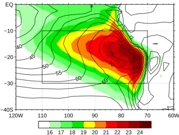
Figure 1 displays the annual-mean adjusted low cloud amount over the Southeast Pacific, with the annual-mean LTS climatology superimposed. Low cloud amount exceeds 60 % over a large region with a spatial extent of roughly two thousand km, and approaches 75 % near Peruvian and north-ern Chilean coast. It decreases toward the equator and mid-latitudes, as higher clouds associated with deep convection to the north and deep frontal clouds to the south predom-inate. This spatial pattern generally matches that of LTS. Maximum LTS values are seen just offshore of the Peruvian and northern Chilean coast. LTS then decreases westward, equatorward and poleward. The low cloud maximum is sev-eral hundred km northwest of the LTS maximum. In light of the prevailing southeast trade winds here, this is downwind of the LTS maximum. This feature suggests low cloud is not in equilibrium with local LTS, but instead is most tightly associated with LTS values 1–2 days upwind. This is consis-tent with the results of mixed-layer model studies (Schubert et al., 1979b).
This massive low cloud deck is present year-round, though it exhibits a modest seasonal cycle. Figure 2 shows the sea-sonal cycles of adjusted and unadjusted low cloud, as well as middle and high cloud, averaged over the oceanic grids within the box shown in Fig. 1. High cloud amount is neg-ligible throughout the year. However, the middle cloud is present in all months. In austral spring (SON) middle cloud increases somewhat due to the intrusion of frontal clouds as-sociated with midlatitude storms. This likely obscures low
40
45
50
55
60
65
70
75
120W 110 100 90 80 70 60W
−40S −30 −20 −10 EQ
16 17 18 19 20 21 22 23 24
Fig. 1. Long-term climatology (1983–2002) of lower-tropospheric
stability (LTS,θ700-θ1000, shaded, Unit: K) and the adjusted low cloud amount (contour, Unit: %).
Dec Jan Feb Mar Apr May Jun Jul Aug Sep Oct Nov 0
10 20 30 40 50 60 70 80
Cloud Cover (%)
16 17 18 19 20 21 22 23 24
LTS (
°
K)
Fig. 2. Seasonal cycles of area-averaged (70◦–110◦W, 10◦–30◦S, refer to box of Fig. 1) ISCCP observed low (black bar), middle (gray bar), high (white bar), adjusted low (solid line with open circle) cloud amount and LTS (dashed line with open square).
Figure 2 shows that LTS also has a distinct seasonal cycle. It rises to a peak of around 20.5 K in October and reaches its minimum of about 18.5 K in March. The seasonal cycles of low cloud cover and LTS are generally in phase, though the seasonal variation of LTS is more sinusoidal than that of low cloud, which flattens out as it reaches its maximum. This suggests the relationship between low cloud cover and LTS weakens as low cloud amount rises above about 60 %, or alternatively, LTS rises above about 19–20 K.
4 Interannual variability
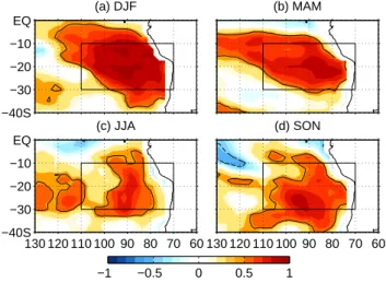
In this section, we examine the relationship between LTS and low cloud cover on interannual timescales. To simplify the analysis and focus on temporal rather than spatial vari-ability, we will examine cloud anomalies averaged over the oceanic grids within the box in Fig. 1. To demonstrate that these area-averaged anomalies are broadly representative of coherent cloud variability in the region for each season, we correlated them with cloud anomalies at every ISCCP grid point (Fig. 3). Large and statistically significant correla-tions are seen at most locacorrela-tions within the averaging box for each season. The geographical coherence of cloud anoma-lies varies somewhat by season, with DJF being the most co-herent across the box and JJA being the least. We further performed an Empirical Orthogonal Function (EOF) analy-sis (not shown) of the low cloud anomalies over the South-east Pacific for all seasons and found that the leading modes are very similar to the patterns seen in Fig. 3 for the four sea-sons. This seasonal variation may reflect some seasonality in the shape of the cloud deck. In any event, Fig. 3 shows that the area-averaged anomalies are reasonable surrogates for lo-cal cloud anomalies that are in phase with one another over a large swath of the region for each season.
Having demonstrated the representativeness of the averaged timeseries, we show a scatterplot of monthly, area-averaged LTS versus low cloud amount, color-coded by cal-endar months in Fig. 4. Smaller low cloud values generally correspond to smaller LTS values, and the associations with the various months of the year are consistent with the phas-ing of the seasonal cycles of LTS and low cloud shown in Fig. 2. The data points in Fig. 4 behave differently depend-ing on their relationship with the long-term LTS climatology. The points whose LTS values are less than the climatology (LTS<LTS) show a pronounced linear correlation between low cloud amount and LTS (correlation coefficientr=0.56), with a 1 K increase of LTS corresponding roughly to a 5.4 % increase in low cloud amount. Conversely, the points to the right of the dotted line (LTS>LTS) do not exhibit such a strong linear relationship (r=0.23), with the regression co-efficient reduced to about 1.6 % per K significantly. Thus the association between LTS and low cloud cover practically disappears for anomalously high LTS values.
(a) DJF
−40S −30 −20 −10 EQ
(c) JJA
130 120 110 100 90 80 70 60 −40S
−30 −20 −10 EQ
(b) MAM
(d) SON
130 120 110 100 90 80 70 60
−1 −0.5 0 0.5 1
Fig. 3. Correlation of seasonal mean, area-averaged adjusted low
cloud amount with adjusted low cloud amount at each grid point for season (a) DJF, (b) MAM, (c) JJA and (d) SON. Contour line denoting the 95 % significance level using the Student-t test is high-lighted. The area of averaging is shown as a box, and is identical to the box in Fig. 1.
16 17 18 19 20 21 22
30 35 40 45 50 55 60 65 70 75
LTS (K)
Cloud Cover (%)
: 5.44x−42.8 : 1.63x+33.0
DecJanFebMarAprMayJun Jul AugSepOctNov
Fig. 4. Scatterplot of the monthly area-averaged (70◦–110◦W, 10◦–30◦S, refer to the box of Fig. 1) LTS versus monthly area-averaged adjusted low cloud amount from 1983 to 2002, color-coded by calendar months. The dotted line denotes the annual mean LTS = 19.4 K. The solid (dashed) line denotes linear least-square re-gression line when LTS<(>)LTS.
Table 1. Slopes (Unit: % per K) of linear regression and correlation coefficients between area-averaged (70◦–110◦W, 10◦–30◦S) adjusted low cloud amount and LTS on interannual and daily timescales grouped by different seasons. Correlation coefficients with significance at the 95 % level using the Student-t test are bolded.
Slope (corr.) DJF MAM JJA SON
interannual 4.45 (0.85) 3.06 (0.61) 0.66 (0.19) 3.02 (0.47) daily (2000, La Ni˜na) 6.34 (0.78) 2.48 (0.38) 1.30 (0.17) 2.41 (0.35) daily (2001, neutral) 5.39 (0.56) 0.76 (0.09) 1.33 (0.22) 2.06 (0.31) daily (1998, El Ni˜no) 4.97 (0.48) 2.76 (0.38) 2.25 (0.38) 3.47 (0.51)
and low cloud cover during austral winter and spring (JJA and SON). This could partly account for the weaker asso-ciation between LTS and low cloud cover for the points to the right of the dotted line in Fig. 4. However, it turns out that the purely internally-generated component of the vari-ability in Fig. 4 is characterized by a very similar seasonal-ity in the LTS–low cloud relationship. We demonstrate this by calculating the seasonal means of area-averaged LTS and low cloud amount for each year and then stratifying the data by season, creating a timeseries of interannual variability for each season. Table 1 presents the resulting slopes of linear regression coefficients and correlation coefficients. In austral summer (DJF), year-to-year variations of low cloud amount are highly correlated with LTS variability (r=0.85). Ev-ery 1 K increase in atmospheric stability is associated with about a 4.5 % increase in low cloud amount. The fall season (MAM) exhibits a somewhat weaker relationship between stability and low cloud amount, with a smaller sensitivity of cloud amount to LTS (3.1 % per K), and a lower though still significant correlation coefficient (r=0.61). In winter (JJA) and spring (SON), the association between LTS and cloud becomes less significant, particularly in JJA.
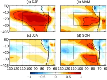
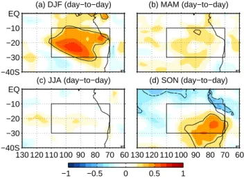
To explore the spatial relationships underpinning the LTS– low cloud statistics of internally-generated interannual vari-ability in Table 1, we calculate for each season correlations between seasonal-mean, area-averaged marine low cloud amount and local LTS for the entire Southeast Pacific. Fig-ure 5a displays the corresponding map for DJF. A zone of strong correlation emerges just off the coast of southern Peru and northern Chile. There is a remarkable similarity between this figure and the characteristic geographical structure of the area-averaged DJF cloud timeseries shown in Fig. 3a. This indicates that the interannual DJF variations of the entire cloud deck arise from a remarkably simple mechanism. They may be understood as a spatially-coherent response to co-located regional-scale LTS forcing. In contrast, Fig. 5b for MAM shows that significant relationships between LTS and area-averaged low cloud amount appear only in the upwind quadrant of the target area of cloud averaging, near the north-ern Chilean coast. If Fig. 3b is an approximate representation of the geographical structure of the area-averaged low cloud MAM timeseries, Fig. 5b suggests these cloud anomalies are generated near the Chilean coast and then advected over the
(a) DJF
−40S −30 −20 −10 EQ
(c) JJA
130 120 110 100 90 80 70 60 −40S
−30 −20 −10 EQ
(b) MAM
(d) SON
130 120 110 100 90 80 70 60
−1 −0.5 0 0.5 1
Fig. 5. Correlation of seasonal mean, area-averaged adjusted low
cloud amount with LTS at each grid point for season (a) DJF,
(b) MAM, (c) JJA and (d) SON. Contour line denoting the 95 %
significance level using the Student-t test is highlighted.
remainder of the averaging region. However, the associated LTS anomalies do not survive. Consistent with the statis-tics in Table 1, the correlation practically disappears for both JJA and SON for the whole Southeast Pacific (Fig. 5c and d), except for some small positive correlations in the southeast portion of the target area in SON.
−1 −0.5 0 0.5 1 500
600
700
775
850
925
1000
hPa
(a) Correlation
DJF MAM JJA SON
−20 −10 0 10
500
600
700
775
850
925
1000
hPa
% per K (b) Regression
DJF MAM
Fig. 6. Correlation coefficients (a) and regression coefficients
(b) between seasonal mean, area-averaged (refer to the box of
Fig. 1) adjusted low cloud amount and temperatures at each ver-tical level colored by seasons. Regression coefficients in only DJF and MAM are shown in (b) considering the correlation coefficients
(a) are only significant through the column in those two seasons.
The dotted lines in (a) denote the 95 % significance level using the Student-t test for interannual cases. The red dashed line denotes the daily analog for DJF of the year 2000.
between low cloud cover and LTS (Table 1) is higher than the correlations between low cloud cover and either constituent part of LTS, so that variability at both levels must be taken into account to maximize the association between cloud and atmospheric thermal properties. In MAM and SON, in con-trast, only the near surface temperature is significantly corre-lated with low cloud amount, while the free atmospheric tem-perature is not. This suggests the MAM/SON LTS anomalies seen in Fig. 5b and d along the northern Chilean coast have
(a) DJF
−40S −30 −20 −10 EQ
(c) JJA
130 120 110 100 90 80 70 60 −40S
−30 −20 −10 EQ
(b) MAM
(d) SON
130 120 110 100 90 80 70 60
−1 −0.5 0 0.5 1
Fig. 7. Correlation of daily area-averaged adjusted low cloud amount with that at each grid point for (a) DJF, (b) MAM, (c) JJA and (d) SON of 2000. Contour line denoting the 95 % significance level using the Student-t test is highlighted.
their origins mainly in SST variability. A mainly oceanic origin for these MAM and SON LTS anomalies would also explain why they do not survive as the low cloud anomalies associated with them are advected into the remainder of the averaging region. Consistent with Fig. 5, low cloud amount anomalies are largely uncorrelated with atmospheric temper-ature anomalies throughout the lower troposphere in JJA.
The magnitudes of the cloud anomalies associated with a 1 K change in temperature at the various levels of the lower troposphere are shown in Fig. 6b. For both DJF and MAM (solid lines), the values are larger near the surface than around 700 hPa. Thus low cloud amount appears to be more sensitive to the surface temperature component of LTS. How-ever, surface temperature variability levels are also lower than at 700 hPa. The standard deviation of DJF (MAM) tem-perature is 0.27 K (0.31 K) at 1000 hPa, while it is 0.68 K (0.50 K) at 700 hPa. We have seen that in DJF the sensitiv-ity to the surface temperature component of LTS is approx-imately twice as large as the sensitivity to the 700 hPa com-ponent. Since the temperature variability levels are roughly twice as large at 700 hPa, the 700 hPa level may become com-petitive with the surface in generating a cloud anomaly sim-ply by exhibiting more variability.
5 Daily variability
16 18 20 22 20
30 40 50 60 70 80
LTS (K)
Cloud Cover (%)
(a)LaN ina˜ (2000)
DJF: 6.3x−62.7 JJA: 1.3x+37.7
D J F M A M J J A S O N
16 18 20 22
20 30 40 50 60 70 80
LTS (K)
Cloud Cover (%)
DJF: 5.0x−40.6 JJA: 2.5x+15.5 (b)E lN ino˜ (1998)
Fig. 8. Scatterplot of the daily area-averaged (refer to the box in
Fig. 1) LTS versus daily area-averaged adjusted low cloud amount from all seasons of La Ni˜na year 2000 (a) and El Ni˜no year 1998
(b), colored by the calendar months. Solid lines denotes best-fit
linear regression for austral summer (DJF) and dashed for winter (JJA) of 2000 (a) and 1998 (b).
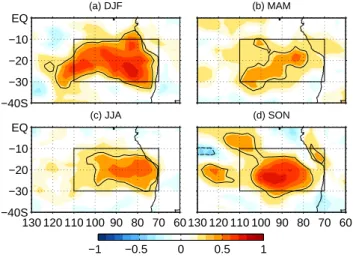
at each grid point for each season for the year 2000. Statisti-cally significant positive correlations are evident in each sea-son over a large portion of the averaging area. Compared to Fig. 3, the correlations are somewhat smaller than their inter-annual counterparts. Low cloud day-to-day variability is less geographically coherent than interannual variability, which is associated with synoptic coastally trapped perturbations. We discuss this further in the context of Fig. 10. In general,
(a) DJF (day−to−day)
−40S −30 −20 −10 EQ
(c) JJA (day−to−day)
130 120 110 100 90 80 70 60 −40S
−30 −20 −10 EQ
(b) MAM (day−to−day)
(d) SON (day−to−day)
130 120 110 100 90 80 70 60
−1 −0.5 0 0.5 1
Fig. 9. Correlation of daily area-averaged adjusted low cloud amount with daily LTS at each grid point for (a) DJF, (b MAM,
(c) JJA and (d) SON of 2000. Contour line denoting the 95 %
sig-nificance level using the Student-t test is highlighted.
however, the area-averaged low cloud represents a large frac-tion of cloud variability in the region on daily timescales for each season.
We then explore whether the seasonal dependence of the LTS–low cloud relationship seen on interannual timescales also holds on daily timescales. Table 1 shows the corre-lation coefficients between daily mean, area-averaged low cloud cover and LTS grouped by different seasons for the year 2000. DJF stands out as the season in which day-to-day low cloud amount is best-correlated with LTS (r=0.78). MAM and SON shows weakened correlation (r=0.38 and 0.35) while in JJA the linear relationship disappears. This seasonal dependence is nearly identical to that seen for in-terannual timescales. This familiar pattern is also seen in Fig. 8a, which shows a scatterplot of daily area-averaged LTS versus low cloud cover for the year 2000, colored by calendar months and with linear least-square regression lines for DJF and JJA superimposed. This figure is qualitatively similar to its internnual variability counterpart (Fig. 4). However, for DJF daily anomalies, every 1 K change in LTS is associated with a 6.3 % low cloud amount change. This is larger than the corresponding DJF value of 4.5 % per K for interannual timescales. We discuss these quantitative differences in the LTS–low cloud relationship on the two timescales further in Sect. 6.
LTS and low cloud anomalies are geographically coherent over the target area. The dashed red line in Fig. 6a reveals that anomalies both near the surface and at 700–775 hPa lev-els contribute to the DJF LTS anomalies associated with low cloud. Daily (Fig. 6b, dashed line) DJF low cloud anomalies are more sensitive to temperatures in the free atmosphere and near the surface compared to the interannual case. As in the interannual case, the sensitivity to conditions near the surface is significantly greater than to conditions above the boundary layer. The LTS–low cloud relationship weakens in MAM and SON, with statistically significant relationships evident in only part of the target area. In JJA, the linkage between LTS and low cloud amount disappears.
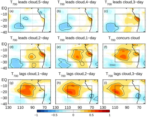
Data with daily resolution allows us to examine the time evolution of synoptic atmospheric variability associated with low cloud anomalies. We do this analysis for DJF, the sea-son with the clearest and most geographically-coherent rela-tionship between LTS and low cloud cover. For the entire Southeast Pacific we calculate the lead-lag correlation be-tween area-averaged low cloud amount with local tempera-ture at the two vertical levels used to calculate LTS. Figure 10 shows the result for atmospheric temperature at 700 hPa. An anomalous warming first appears along the Peruvian and northern Chilean coasts 3–4 days ahead of a positive cloud amount anomaly. The anomalous warming then propagates westward. The propagation continues after the cloud amount peaks, until the warm anomalies move out of the target area 2–3 days later. Figure 11 shows the corresponding correla-tion between area-averaged low cloud cover and temperature near the surface at 1000 hPa in DJF. Anomalous near-surface cooling is persistent in a swath across the lower portion of the target area as the low clouds grow, peak, and decay. Thus the propagating signal seen in Fig. 10 is not evident here. Apparently, the timescales of variability at the two vertical levels are different. This is confirmed by a calculation of the e-folding timescales for the area-averaged temperature at 1000 and 700 hPa, 8–9 and 3–4 days respectively. The longer timescale for the near surface temperature suggests it is strongly affected by SST variability, and exhibits some of the relative sluggishness of ocean surface thermal variability (Manabe and Stouffer, 1996; Hall and Manabe, 1997; Sura et al., 2006). Furthermore, the area-averaged temperatures at 700 hPa and 1000 hPa are uncorrelated (r= −0.09), demon-strating the complete independence of free atmosphere and near surface temperature anomalies. Thus, two independent modes of variability with different spatial and temporal struc-tures, one primarily oceanic and the other primarily atmo-spheric in origin, both contribute to daily LTS variability in DJF.
6 ENSO modulation
The seasonal dependence of the relationship between daily LTS and low cloud anomalies is qualitatively similar to that of the interannual anomalies discussed in Sect. 4.
How-ever, there are unexplained quantitative differences between the two timescales. For example, in DJF a given daily LTS anomaly is associated with a significantly larger low cloud anomaly than in the interannual case. It turns out that this dif-ference can be traced to modulation of the LTS–low cloud re-lationship by the ENSO phenomenon. The analysis of daily variability in Sect. 5 relied on data from the year 2000. This was a La Ni˜na year. Table 1 also shows the LTS–low cloud relationship in neutral (2001) and El Ni˜no (1998) years. The El Ni˜no/La Ni˜na is defined when the 5-month running means of SST anomalies averaged in the ni˜no3.4 region (170◦W– 120◦W, 5◦S–5◦N) exceed 0.4◦C (−0.4◦C) for 6 months or more (Trenberth, 1997). The SST anomalies are calculated using the monthly OISST.v2, deviated from the 1971–2000 long-term monthly mean. Comparison of the three years in-dicates the relationship between LTS and low cloud amount on daily timescales depends on the large-scale state of the tropical Pacific. In DJF, a 1 K increase of daily LTS is as-sociated with 5.0 %, 5.4 % and 6.3 % increases in low cloud amount for El Ni˜no, neutral and La Ni˜na years respectively. Thus low cloud anomalies associated with LTS changes are larger and low cloud cover is better correlated with LTS the further the ocean-atmosphere system is from the El Ni˜no phase of the ENSO cycle. A visual comparison of Fig. 8a and b shows just how qualitatively different the LTS–low cloud relationship is during the two extreme phases of the ENSO cycle. During an El Ni˜no year, the cluster of DJF points re-sembles the cluster of JJA points for the La Ni˜na year, and overlaps significantly with the clusters of the other seasons.
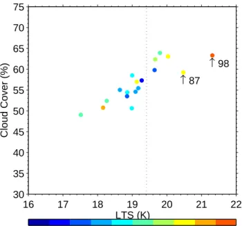
The ENSO modulation of the LTS–low cloud relationship on daily timescales raises the question of whether the imprint of the ENSO phenomenon may be seen in the LTS–low cloud relationship on interannual timescales. In Fig. 12 we show a scatterplot of the seasonal mean, area-averaged LTS versus low cloud amount for only the DJF season, colored by the DJF mean ni˜no3.4 index. Note that the slope of the linear regression corresponding to this scatterplot is shown in Ta-ble 1. In general, the higher ENSO index years tend to be on the right side of the distributions, so that warm ENSO events are associated with higher LTS values. There are exceptions. For example, there is an El Ni˜no event that has a relatively low LTS of around 18 K, the result of increased tempera-ture in both the lower troposphere and the near surface. Fig-ure 12 shows two warm ENSO events of the record, namely the 1987 and 1998 El Ni˜no events, are visible outliers. Al-though these two events are characterized by very high LTS in the Southeast Pacific, the accompanying low cloud val-ues are not correspondingly high. Including these two events significantly flattens the slope of the LTS–low cloud regres-sion on interannual timescales. Without them, the slope of the LTS–low cloud regression increases from 4.5 % per K to 5.6 % per K, comparable to the corresponding values on daily timescales for a neutral ENSO year (Table 1, year 2001).
(a)
T
700 leads cloud,5−day
−40 −30 −20 −10 EQ
(d)
T
700 leads cloud,2−day
−40 −30 −20 −10 EQ
(g)
T
700 lags cloud,1−day
130 110 90 70
−40 −30 −20 −10 EQ
(b)
T
700 leads cloud,4−day
(e)
T
700 leads cloud,1−day
(h)
T
700 lags cloud,2−day
130 110 90 70
(c)
T
700 leads cloud,3−day
(f)
T
700 concurs cloud
(i)
T
700 lags cloud,3−day
130 110 90 70
−1 −0.5 0 0.5 1
Fig. 10. Lead-lag correlation of daily area-averaged adjusted low cloud amount with daily temperature at 700 hPa at each grid point for
austral summer (DJF) of 2000. Contour line denoting the 95 % significance level using the Student-t test is highlighted.
(a)
T
1000 leads cloud,5−day
−40 −30 −20 −10 EQ
(d)
T
1000 leads cloud,2−day
−40 −30 −20 −10 EQ
(g)
T
1000 lags cloud,1−day
130 110 90 70
−40 −30 −20 −10 EQ
(b)
T
1000 leads cloud,4−day
(e)
T
1000 leads cloud,1−day
(h)
T
1000 lags cloud,2−day
130 110 90 70
(c)
T
1000 leads cloud,3−day
(f)
T
1000 concurs cloud
(i)
T
1000 lags cloud,3−day
130 110 90 70
−1 −0.5 0 0.5 1
16 17 18 19 20 21 22 30
35 40 45 50 55 60 65 70 75
LTS (K)
Cloud Cover (%)
↑ 87
↑ 98
24 24.5 25 25.5 26 26.5 27 27.5 28 28.5
Fig. 12. Scatterplot of the area-averaged (70◦–110◦W, 10◦–30◦S) LTS versus adjusted low cloud amount for DJF season from 1983 to 2002, colored by the DJF mean ni˜no3.4 index, an indicator of ENSO defined as area-averaged (170◦W–120◦W, 5◦S–5◦N) SST in the tropical Pacific.
21 K, comparable to those typically found in JJA. Low cloud amount also exhibits the reduced sensitivity to LTS charac-teristic of JJA, reducing the slope of the LTS–low cloud re-gression when those points are included in the rere-gression cal-culation. This is consistent with our findings in previous sec-tions: the LTS–low cloud relationship weakens dramatically as LTS increases and reaches a threshold of about 19.5 K. This threshold, normally not breached during DJF, is very commonly breached during strong El Ni˜no events.
7 Discussion and implications
In this study, we examine ISCCP observed low cloud cover variability in the Southeast Pacific and its association with ERA-40 calculated LTS across a spectrum of timescales. First, the seasonal cycles of LTS and low cloud cover are ap-proximately in phase with each other. However, LTS shows a pronounced seasonal cycle with a distinct peak in austral spring (SON), while low cloud amount flattens out when it reaches the maximum in winter (JJA) and spring (SON). The association between LTS and low cloud cover appears to weaken in seasons with high LTS values. When consid-ering the seasonal cycle only, every 1 K anomaly in LTS is associated with about a 5.3 % change in low cloud amount. This value is comparable to, though somewhat smaller than the values of 5.7 % and 5.0 % reported in Klein and
Hart-mann (1993) and Zhang et al. (2009). The seasonal depen-dence of the LTS–low cloud relationship hinted in the sea-sonal cycle analysis is brought into sharp relief through an examination of interannual and daily variability. On both timescales, LTS and low cloud cover are very well correlated in summer (DJF), and both LTS and low cloud anomalies are regionally-coherent. This indicates that even local low cloud variability at this time of year can be understood in terms of the regional-scale LTS–low cloud relationship. Meanwhile, though the regional-scale coherence of cloud deck variabil-ity is also present in winter (JJA), the LTS–low cloud cor-relation substantially weakens. The DJF LTS–low cloud re-lationship weakens in years with larger ambient LTS values. These years are generally strong El Ni˜no years, in which DJF LTS values are comparable to those typically found in JJA. Thus the LTS–low cloud relationship is strongly modulated by the ENSO phenomenon.
To determine the origin of LTS anomalies closely asso-ciated with internally-generated low cloud cover variabil-ity during austral summer, we examine the relationships be-tween low cloud variability and temperature variability at the surface and above the boundary layer. We find that both lev-els contribute approximately equally to low cloud variability for both interannual and daily timescales. Meanwhile, tem-perature variability at the two levels is essentially uncorre-lated. This indicates the ocean and atmosphere are both inde-pendently involved in generating the variability of the South-east Pacific low cloud deck, highlighting the coupled nature of the climate system in this region. The lack of correlation between the near surface and upper air was also found in ob-servational studies of the Northeast Pacific low cloud cover (Klein et al., 1995; Klein, 1997). This result also raises the possibility of cloud feedbacks related to LTS. For example, if positive LTS and low cloud anomalies persisted long enough to substantially reduce SSTs, this would increase LTS and cloud still further. The potential importance of such a feed-back is further underscored by the fact that on both daily and interannual timescales, DJF low cloud cover is significantly more sensitive to near-surface conditions than to conditions above the boundary layer. In general, our results underscore the important role of the large-scale atmospheric and oceanic conditions (i.e., the physical climate system) in generating internal low cloud variability in the Southeast Pacific.
sub-regions: west of 90◦W and east of 90◦W. West of 90◦W is a cloud transition region where stratiform cloud transi-tions to cumulus, while east of 90◦W is the solid stratiform cloud region. Examination of low cloud’s sensitivity to LTS in the two sub-regions show that the substantially weakened sensitivity to LTS is most obvious east of 90◦W, where the most overcast conditions occur. West of 90◦W, the transition region shows only somewhat weakened sensitivity to LTS. There have been modeling studies on this nonlinear behavior of low cloud sensitivity to LTS. For example, Zhang et al. (2009) used a mixed-layer model to study the low cloud’s nonlinear response to the large-scale divergence. In their Fig. 14, they showed the enhanced large-scale divergence ac-companies larger LTS, and inhibits the growth of low cloud amount. The second explanation is related to the atmospheric synoptic thermal structure important in modulating day-to-day cloud variability (Fig. 10). The synoptic activities are characterized by a westward propagation of thermal anoma-lies first originating from the coasts of southern Peru and northern Chile to the open ocean. These were also found in previous modeling studies (Garreaud and Rutllant, 2003) and in the recent Variability of the American Monsoon (VAMOS) Ocean-Cloud-Atmosphere-Land Study Regional Experiment (VOCALS-REx, Wood et al. (2010)) field campaign (Rahn and Garreaud, 2010). This may be attributable to zonal tem-perature advection induced by the land-sea thermal contrast and land-deflected synoptic storms. So the occasional off-shore flow from land brings very warm and dry air over the near coastal ocean, leading to very high LTS values but con-ditions too dry for a cloud to form. This might also explain the substantially weakened cloud sensitivity to LTS.
Our studies also show the more regime-independent EIS has very similar relationship with low cloud cover to the LTS–low cloud relationship. The relationship between low cloud cover and LTS or EIS has been invoked in the context of current climate simulations to parameterize the low cloud amount in some weather forecast models (Slingo, 1987) and climate models (Rasch and Kristj´ansson, 1998; Collins et al., 2006) and to understand low cloud cover changes in a warm-ing climate (Stevens and Brenguier, 2009; Bretherton and Hartmann, 2009). And it has been relied on to make pre-dictions about the behavior of low cloud feedback and the implications for future climate change. For example, Miller (1997) suggested that since LTS tends to increase in a warmer climate due to greater atmospheric warming in subtropical regions above the boundary layer than at the surface, low cloud cover will increase, leading to a negative feedback. Our results from the Southeast Pacific indicate that while it may be valid to extrapolate the low cloud cover change in a future climate where LTS increases relying on the cur-rent LTS–low cloud relationship, some caution is warranted. The exact nature of the relationship between LTS and low cloud cover appears to be regime-dependent even during the summer season when the LTS–low cloud relationship is strongest. The overall change in climate associated with
an-thropogenic forcing may be large enough to cause a change during a particular season from one regime to another. Our results also show that during austral winter and spring, most temporal variability in the low cloud deck is consistently unrelated to LTS. Other regional-scale factors must be im-portant in generating low cloud variability, such as tempera-ture advection, the strength of the subtropical high, the sur-face wind and the relative humidity of the cloud layer (Klein et al., 1995; Klein, 1997; George and Wood, 2010; Paine-mal and Zuidema, 2010). Besides the physical meteorologi-cal controls on low cloud, the atmospheric aerosols are also important for cloud formation, particularly the cloud micro-structure (Albrecht, 1989; Bretherton et al., 2004), and po-tentially overall cloud amount. During these seasons, it is difficult to justify relying on the LTS–low cloud relationship to make predictions or statements about the low cloud cover response to anthropogenic forcing in the Southeast Pacific. Meanwhile, this nonlinear LTS–low cloud relationship found in the Southeast Pacific in this study may behave differently in other low cloud regions, another topic for a future study.
Acknowledgements. This research was supported by US National
Science Foundation (NSF-0747533). The authors thank the anonymous reviewers for their helpful and constructive comments that have helped the improvement of this paper. Data used in this study including ERA40, ISCCP, OISST.v2 are made available separately from ECMWF data server, http://data.ecmwf.int, NASA Langley Research Center, http://eosweb.larc.nasa.gov and NOAA Earth System Research Laboratory, http://www.esrl.noaa.gov.
Edited by: B. Albrecht
References
Albrecht, B. A. A.: Aerosols, Cloud Microphysics, and Fractional Cloudiness, Science, 245, 1227–1230, 1989.
Albrecht, B. A., Randall, D. A., and Nicholls, S.: Observations of Marine Stratocumulus Clouds During FIRE, B. Am. Meteorol. Soc., 69, 618–626, 1988.
Bony, S. and Dufresne, J.-L.: Marine boundary layer clouds at the heart of tropical cloud feedback uncertainties in climate models, Geophys. Res. Lett., 32, L20806, doi:10.1029/2005GL023851, 2005.
Bretherton, C. S. and Hartmann, D. L.: Large-scale controls on cloudiness, in: Perturbed Clouds in the Climate System: Their Relationship to Energy Balance, Atmospheric Dynamics and Precipitation, edited by: Heintzenberg, J. and Charlson, R. J., vol. 2 of Strungmann Forum Reports, pp. 217–234, MIT Press., 2009.
Bretherton, C. S., Uttal, T., Fairall, C. W., Yuter, S. E., Weller, R. A., Baumgardner, D., Comstock, K., Wood, R., and Raga, G. B.: The Epic 2001 Stratocumulus Study, B. Am. Meteorol. Soc., 85, 967–977, 2004.
Collins, W. D., Rasch, P. J., Boville, B. A., Hack, J. J., McCaa, J. R., Williamson, D. L., Briegleb, B. P., Bitz, C. M., Lin, S.-J., and Zhang, M.: The Formulation and Atmospheric Simulation of the Community Atmosphere Model Version 3 (CAM3), J. Climate, 19, 2144–2161, 2006.
Garay, M. J., de Szoeke, S. P., and Moroney, C. M.: Com-parison of marine stratocumulus cloud top heights in the southeastern Pacific retrieved from satellites with coincident ship-based observations, J. Geophys. Res., 113, D18204, doi:10.1029/2008JD009975, 2008.
Garreaud, R. and Rutllant, J.: Coastal Lows along the Subtropical West Coast of South America: Numerical Simulation of a Typi-cal Case, Mon. Weather Rev., 131, 891–908, 2003.
Garreaud, R. D., Rutllant, J., Quintana, J., Carrasco, J., and Minnis, P.: CIMAR-5: A Snapshot of the Lower Troposphere over the Subtropical Southeast Pacific, B. Am. Meteorol. Soc., 82, 2193– 2207, 2001.
George, R. C. and Wood, R.: Subseasonal variability of low cloud radiative properties over the Southeast Pacific Ocean, Atmos. Chem. Phys., 10, 4047–4063, doi:10.5194/acp-10-4047-2010, 2010.
Ghate, V. P., Albrecht, B. A., Fairall, C. W., and Weller, R. A.: Cli-matology of Surface Meteorology, Surface Fluxes, Cloud Frac-tion, and Radiative Forcing over the Southeast Pacific from Buoy Observations, J. Climate, 22, 5527–5540, 2009.
Hall, A. and Manabe, S.: Can local linear stochastic theory explain sea surface temperature and salinity variability?, Clim. Dynam., 13, 167–180, doi:10.1007/s003820050158, 1997.
Hartmann, D. L., Ockert-Bell, M. E., and Michelsen, M. L.: The Ef-fect of Cloud Type on Earth’s Energy Balance: Global Analysis, J. Climate, 5, 1281–1304, 1992.
Kawai, H. and Teixeira, J.: Probability Density Functions of Liq-uid Water Path and Cloud Amount of Marine Boundary Layer Clouds: Geographical and Seasonal Variations and Controlling Meteorological Factors, J. Climate, 23, 2079–2092, 2010. Klein, S. A.: Synoptic Variability of Low-Cloud Properties and
Me-teorological Parameters in the Subtropical Trade Wind Boundary Layer, J. Climate, 10, 2018–2039, 1997.
Klein, S. A. and Hartmann, D. L.: The Seasonal Cycle of Low Strat-iform Clouds, J. Climate, 6, 1587–1606, 1993.
Klein, S. A., Hartmann, D. L., and Norris, J. R.: On the Relation-ships among Low-Cloud Structure, Sea Surface Temperature, and Atmospheric Circulation in the Summertime Northeast Pa-cific, J. Climate, 8, 1140–1155, 1995.
Lin, W., Zhang, M., and Loeb, N. G.: Seasonal Variation of the Physical Properties of Marine Boundary Layer Clouds off the California Coast, J. Climate, 22, 2624–2638, 2009.
Lohmann, U. and Lesins, G.: Stronger Constraints on the Anthro-pogenic Indirect Aerosol Effect, Science, 298, 1012–1015, 2002. Mace, G. G., Benson, S., Sonntag, K. L., Kato, S., Min, Q., Min-nis, P., Twohy, C. H., Poellot, M., Dong, X., Long, C., Zhang, Q., and Doelling, D. R.: Cloud radiative forcing at the At-mospheric Radiation Measurement Program Climate Research Facility: 1. Technique, validation, and comparison to satellite-derived diagnostic quantities, J. Geophys. Res., 111, D11S91, doi:10.1029/2005JD005922, 2006.
Manabe, S. and Stouffer, R. J.: Low-Frequency Variability of Sur-face Air Temperature in a 1000-Year Integration of a Coupled Atmosphere-Ocean-Land Surface Model, J. Climate, 9, 376–
393, 1996.
Mansbach, D. K. and Norris, J. R.: Low-Level Cloud Variability over the Equatorial Cold Tongue in Observations and Models, J. Climate, 20, 1555–1570, 2007.
Miller, R. L.: Tropical Thermostats and Low Cloud Cover, J. Cli-mate, 10, 409–440, 1997.
Minnis, P., Heck, P. W., Young, D. F., Fairall, C. W., and Snider, J. B.: Stratocumulus Cloud Properties Derived from Simultane-ous Satellite and Island-based Instrumentation during FIRE, J. Appl. Meteorol., 31, 317–339, 1992.
Painemal, D. and Zuidema, P.: Microphysical variability in Southeast Pacific Stratocumulus clouds: synoptic conditions and radiative response, Atmos. Chem. Phys., 10, 6255–6269, doi:10.5194/acp-10-6255-2010, 2010.
Rahn, D. A. and Garreaud, R.: Marine boundary layer over the subtropical Southeast Pacific during VOCALS-REx - Part 2: Synoptic variability, Atmos. Chem. Phys., 10, 4507–4519, doi:10.5194/acp-10-4507-2010, 2010.
Ramanathan, V., Cess, R. D., Harrison, E. F., Minnis, P., Barkstrom, B. R., Ahmad, E., and Hartmann, D.: Cloud-Radiaive Forcing and Climate-Results from the Earth Radiation Budget Experi-ment, Science, 243, 57–63, 1989.
Randall, D. A., Coakley, J. A., Lenschow, D. H., Fairall, C. W., and Kropfli, R. A.: Outlook for Research on Subtropical Marine Stratification Clouds, B. Am. Meteorol. Soc., 65, 1290–1301, 1984.
Rasch, P. J. and Kristj´ansson, J. E.: A Comparison of the CCM3 Model Climate Using Diagnosed and Predicted Condensate Pa-rameterizations, J. Climate, 11, 1587–1614, 1998.
Reynolds, R. W., Rayner, N. A., Smith, T. M., Stokes, D. C., and Wang, W.: An Improved In Situ and Satellite SST Analysis for Climate, J. Climate, 15, 1609–1625, 2002.
Rossow, W. B. and Schiffer, R. A.: ISCCP Cloud Data Products, B. Am. Meteorol. Soc., 72, 2–20, 1991.
Rossow, W. B. and Schiffer, R. A.: Advances in Understanding Clouds from ISCCP, B. Am. Meteorol. Soc., 80, 2261–2287, 1999.
Rozendaal, M. A. and Rossow, W. B.: Characterizing Some of the Influences of the General Circulation on Subtropical Marine Boundary Layer Clouds, J. Atmos. Sci., 60, 711–728, 2003. Rozendaal, M. A., Leovy, C. B., and Klein, S. A.: An
Observa-tional Study of Diurnal Variations of Marine Stratiform Cloud, J. Climate, 8, 1795–1809, 1995.
Schubert, W. H., Wakefield, J. S., Steiner, E. J., and Cox, S. K.: Marine Stratocumulus Convection. Part I: Governing Equations and Horizontally Homogeneous Solutions, J. Atmos. Sci., 36, 1286–1307, 1979a.
Schubert, W. H., Wakefield, J. S., Steiner, E. J., and Cox, S. K.: Marine Stratocumulus Convection. part II: Horizontally Inhomo-geneous Solutions, J. Atmos. Sci., 36, 1308–1324, 1979b. Slingo, J. M.: The Development and Verification of a Cloud
Pre-diction Scheme for the ECMWF Model, Q. J. Roy. Meteor. Soc., 113, 899–927, 1987.
Stephens, G. L.: Cloud Feedbacks in the Climate System: A Critical Review, J. Climate, 18, 237–273, 2005.
Strungmann Forum Reports, pp. 173–196, MIT Press., 2009.
Sura, P., Newman, M., and Alexander, M. A.: Daily to Decadal Sea Surface Temperature Variability Driven by State-Dependent Stochastic Heat Fluxes, J. Phys. Oceanogr., 36, 1940–1958, doi:10.1175/JPO2948.1, 2006.
Teixeira, J., May, P., Flatau, M., and Hogan, T. F.: SST sensitivity of a global ocean-atmosphere coupled system to the parameteri-zation of boundary layer clouds, J. Mar. Sys., 69, 29–36, 2008. Trenberth, K. E.: The Definition of El Ni˜no, B. Am. Meteorol. Soc.,
78, 2771–2777, 1997.
Uppala, S. M., Kallberg, P. W., Simmons, A. J., Andrae, U., Bech-told, V. D., Fiorino, M., Gibson, J. K., Haseler, J., Hernandez, A., Kelly, G. A., Li, X., Onogi, K., Saarinen, S., Sokka, N., Al-lan, R. P., Andersson, E., Arpe, K., Balmaseda, M. A., Beljaars, A. C. M., Van De Berg, L., Bidlot, J., Bormann, N., Caires, S., Chevallier, F., Dethof, A., Dragosavac, M., Fisher, M., Fuentes, M., Hagemann, S., Holm, E., Hoskins, B. J., Isaksen, L., Janssen, P. A. E. M., Jenne, R., McNally, A. P., Mahfouf, J. F., Morcrette, J. J., Rayner, N. A., Saunders, R. W., Simon, P., Sterl, A., Tren-berth, K. E., Untch, A., Vasiljevic, D., Viterbo, P., and Woollen, J.: The ERA-40 Re-analysis, Q. J. Roy. Meteor. Soc., 131, 2961– 3012, doi:10.1256/qj.04.176, 2005.
Wood, R. and Bretherton, C. S.: On the Relationship between Strati-form Low Cloud Cover and Lower-Tropospheric Stability, J. Cli-mate, 19, 6425–6432, 2006.
Wood, R., Mechoso, C. R., Bretherton, C. S., Weller, R. A., Huebert, B., Straneo, F., Albrecht, B. A., Coe, H., Allen, G., Vaughan, G., Daum, P., Fairall, C., Chand, D., Gallardo Klen-ner, L., Garreaud, R., Grados, C., Covert, D. S., Bates, T. S., Krejci, R., Russell, L. M., de Szoeke, S., Brewer, A., Yuter, S. E., Springston, S. R., Chaigneau, A., Toniazzo, T., Min-nis, P., Palikonda, R., Abel, S. J., Brown, W. O. J., Williams, S., Fochesatto, J., Brioude, J., and Bower, K. N.: The VA-MOS Ocean-Cloud-Atmosphere-Land Study Regional Experi-ment (VOCALS-REx): goals, platforms, and field operations, Atmos. Chem. Phys., 11, 627–654, doi:10.5194/acp-11-627-2011, 2011.
Xu, H., Xie, S.-P., and Wang, Y.: Subseasonal Variability of the Southeast Pacific Stratus Cloud Deck, J. Climate, 18, 131–142, 2005.
Zhang, G. J., Vogelmann, A. M., Jensen, M. P., Collins, W. D., and Luke, E. P.: Relating Satellite-Observed Cloud Prop-erties from MODIS to Meteorological Conditions for Ma-rine Boundary Layer Clouds, J. Climate, 23, 1374–1391, doi:10.1175/2009JCLI2897.1, 2010.