Integrated Inventory Model With Fuzzy Order Quantity And Fuzzy Shortage Quantity

(1)

Abstract

—

_{This paper investigates an integrated inventory} model with fuzzy order quantity and fuzzy shortage quantity. We express order quantity and shortage quantity as the normal triangular fuzzy numbers and then we will find the membership function of fuzzy cost and its centroid.We find that the estimated value of the total cost in the fuzzy sense is higher than in the crisp model.

Index Terms_{— fuzzy inventory, fuzzy cost, buyer, vendor,} membership function.

I. INTRODUCTION

In traditional inventory management systems, the economic lot size (E.L.S) for a vendor and a buyer are managed independently, that is, the vendor and buyer find their own optimal order quantity. As a result, the E.L.S of buyer may not result in an optimal policy for the vendor and vice-versa. To overcome this problem, researchers have studied joint economic lot size (J.E.L.S) model where the joint total relevant cost (J.T.R.C) for the buyer as well as the vendor has been optimized. Goyal first introduced an integrated inventory policy for a single supplier and a single customer and derived the minimum joint variable cost for the supplier and the customer [1]. Banerjee introduced the J.E.L.S model for a single vendor and a single customer and

Mona Ahmadi-Rad is working as project management expert at Engineering Research Center of Eastern Azarbayjan. Her research has focused on modeling production management problems in both deterministic and fuzzy situation. Mrs. Ahmadi-Rad earned a bachelor's degree in industrial engineering from K.N.Toosi University of Technology, Tehran-IRAN. She is now working on her thesis in order to earn a master's degree in industrial engineering.Tell: +9821-88674843

Email: rad983@gmail.com

Dr. Farid Khoshalhan is an associated Professor in Industrial Engineering and Information Technology at Faculty of Industrial Engineering, K.N.Toosi University of Technology, Tehran-IRAN. His research and client work has focused on inventory and production management, evolutionary algorithms, performance and productivity management and e-commerce. Dr. Khoshalhan earned a bachelor's degree in industrial technology from Iran University of Science and Technology, a master's and PhD in industrial engineering from Tarbiat Modarres University in IRAN. Tell:+9821-88674843

Email: khoshalhan@kntu.ac.ir

obtained the minimum joint total relevant cost for both buyer and vendor at the same time with the assumption that the vendor makes the production set up every time the buyer places an order and supplies on a lot for lot basis [2]. Goyal modified Banerjee's [2] paper on the assumption that vendor may possibly produce a lot size that may supply an integer number of orders to the buyer [3]. Lu relaxed the assumption of Goyal [3] and developed a model with the assumption that the vendor can ship a subbatch to the supplier even before the entire batch is completed [4]. Goyal provided an alternative shipment policy where all the subbatches are not necessarily of same size [5].

Recently, fuzzy concepts have been introduced in the economic order quantity (E.O.Q) models. Zadeh showed the intention of accommodating uncertainty in the non stochastic sense rather than the presence of random variables [6]. Sommer applied fuzzy dynamic programming to an inventory and production-scheduling problem in which the management wishes to fulfill a contract for providing a product and then withdraw from the market [7]. Park examined the E.O.Q model in the fuzzy set theoretic perspective associating the fuzziness with the cost data [8]. Yao and Lee used extension principle to solve E.O.Q model with shortage. They fuzzified the order quantity into triangular fuzzy number, trapezoidal fuzzy number and got the optimal solution in the fuzzy sense [9]-[10]. Later, Chang et al. fuzzified the shortage quantity into triangular fuzzy number and the order quantity was a positive real variable and then deduced the membership function of the fuzzy total cost and its centroid [11]. Wu & Yao fuzzified both order quantity and shortage quantity into triangular fuzzy numbers and got the centroid of fuzzy total cost [12]. For the first time, Mahata et al. investigated the J.E.L.S model for both buyer and vendor in fuzzy sense. In this paper they have extended Banerjee,s [2] J.E.L.S model with the assumption that the order quantity for the buyer/vendor is fuzzy variable[13].

In this article, we use from Mahata et al. [13] and Wu & Yao [12] models and investigate an integrated inventory model with fuzzy order quantity and fuzzy shortage quantity that these are a normal triangular fuzzy number. First in section II, we introduce the assumptions and notations of the model and then in section III, we model a fuzzy total cost for the buyer and vendor at the same time, then obtain a membership function of the fuzzy total cost and its centroid. In section IV, we solve an example and then we summarize the conclusions in section V.

Integrated Inventory Model With Fuzzy Order

Quantity And Fuzzy Shortage Quantity

(2)

II. ASSUMPTIOINS AND NOTATIONS

Following assumptions and notations are considered:

A. assumptions

1) The demand rate and production rate are deterministic.

2) Manufacturing set-up cost, ordering cost, unit inventory holding cost for the vendor and the buyer, are known.

3) Single vendor and single buyer are considered.

4) There is a single product.

5) Shortage is allowed for buyer and fully backordered.

6) The vendor makes the production set up every time the buyer places an order and supplies on a lot for lot basis.

7) Order quantity and shortage quantity are normal triangular fuzzy numbers.

B. notations

D: Annual constant demand

P: Vendor's annual constant rate of production

CV: The unit production cost

CP: The unit purchase cost paid by the purchaser A: The purchaser's ordering cost per order

S: The vendor's setup cost per setup

r: The annual inventory carrying cost per dollar invested in stocks

π: The shortage cost per unit quantity per year

q: The order quantity

b

:The shortage quantity

III. THE MEMBERSHIP FUNCTION AND THE CENTROID OF FUZZY TOTAL COST

First we consider a crisp sense. Thus, Joint total relevant cost by considering shortage, is as follow

b rc q

b rc c c p D r q A s q D b q

F p

p p

v − ⋅

⋅ + + + ⋅ ⋅ + + ⋅ =

2 ) ( ) (

2 ) ( ) , (

2

π

₍₁₎

Therefore the optimal solution in crisp case is

* *

q rc

rc b

p

p _⋅

+ =

π

(2)

2 *

) ( ) ( ) (

) ( ) ( 2

p p

p v

p

rc rc

c c p D r

rc A s D q

− + ⋅ + ⋅

+ ⋅ + ⋅ =

π

π (3)

) (

) ( ) ( ) (

) ( 2 ) , (

2

*

* _π

π

+

⎥ ⎦ ⎤ ⎢

⎣

⎡ _⋅ ₊ _⋅ ₊ ₋

⋅ + ⋅ =

p

p p

p v

rc

rc rc

c c p D r A s D b q

F (4)

Equation (1) and its derivatives have been obtained under the assumption that all the lead time (i.e., the period from

the ordering time to the arrival time) in each cycle are the same. In the reality, such as the traffic condition may vary as well as other situations may affect the lead time among each cycle. Hence in (1) we cannot assume the lead time are all the same in each cycle. This will affect to the certainty of order quantity q and shortage quantity b too. Therefore we shall fuzzify both q and b at the same time, i.e., using a triangular fuzzy number ~q =(q₁,q₀,q₂)

and q

rc rc b

p p _~

~ _⋅

+ =

π .

So

⎪ ⎪ ⎪

⎩ ⎪ ⎪ ⎪

⎨ ⎧

≤ ≤ −

−

≤ ≤ −

−

=

otherwise q q q q

q q q

q q q q

q q q

q

, 0

, ,

)

( ₀ ₂

0 2

2

0 1

1 0

1

~

μ (5)

where0≺q₁≺q₀ ≺q₂; q₁,q₀,q₂are unknown.

For deffuzification , we use the centroid method. Therefore, the centroid of

q

~

is

3 )

( ) (

) ~

( 1 0 2

~ ~

q q q

dx x

dx x x

q c

q q

+ + = =

∫

∞

∞ − ∞

∞ −

μ μ

(6)

where c(q~) denotes the estimated value of the order quantity in the fuzzy sense.

From q

rc rc b

p p

. )

( +π

= and the Extension Principle, we have

⎪ ⎪ ⎪ ⎪ ⎪

⎩ ⎪ ⎪ ⎪ ⎪ ⎪

⎨ ⎧

+ ≤ ≤ + −

⋅ + ⋅ − ⋅

+ ≤ ≤ + −

⋅ ⋅ − + ⋅

=

otherwise

q rc

rc b q rc

rc

q q rc

rc b q rc

q rc

rc b q rc

rc

q q rc

q rc rc b

b

p p p

p p

p p p

p p

b

0

) (

)

( 0 2

0 2 2

0 1

1 0

1

~

π π

π

π π

π

μ

(7)

The centroid of

b

~

, by (7) is

)) ~ ( ) ( ) (

) ( 3 1 ) ~

( ₁ ₀ ₂ C q

rc rc q

q q rc

rc b

C

p p

p

p _⋅

+ = + + ⋅ + ⋅ =

π

(8)

(3)

Property 1. The minimum total cost F(q,b) with respect to

q, b is the same as the minimum total cost

) . , ( ) ( q rc rc q F q G p p π +

= with respect to q and _._q

rc rc b p p π + = . q q b

q

G

q

G

b

q

F

b

q

F

≺ ≺ ≺ 0 * * * * 0

)

(

min

)

(

)

,

(

)

,

(

min

=

With respect to property 1, we replace _._q

rc rc b p p π +

= in (1).

Therefore, we will have

) ( 2 ) ( ) ( 2 ) ( ) ( 2 π + ⋅ − + ⋅ ⋅ + + ⋅ = p p p v rc q rc c c p D r q A s q D q

G

(9)

Let

G

(

q

)

=

z

, then the roots of

G

(

q

)

=

z

are

[

2

]

* 2

2

1 ( )

) ( ) ( ) ( ) ( )

( z z Gq

rc rc c c p D r rc z d p p p v

p _⋅ ₋ ₋

⎥ ⎦ ⎤ ⎢ ⎣ ⎡ _⋅ ₊ _⋅ ₊ ₋ + = π

π

(10)

and

[

2

]

* 2

2

2 ( )

) ( ) ( ) ( ) ( )

( z z Gq

rc rc c c p D r rc z d p p p v

p _⋅ ₊ ₋

⎥ ⎦ ⎤ ⎢ ⎣ ⎡ _⋅ ₊ _⋅ ₊ ₋ + = π

π (11)

From

G

(

q

)

=

z

and the Extension Principle, we have the membership function of the fuzzy total cost

G

(

q

~

)

as follow

[

]

⎪ ⎪ ⎩ ⎪ ⎪ ⎨ ⎧ ≥ = otherwise 0 ) q ( G z if )) z ( d ( )), z ( d ( max ) z ( * 2 q ~ 1 q~ ) q ~ ( G μ μ

μ (12)

In order to solve (12), we use the Table I and equations (13)-(25).

In table I, we consider the different position of d₁(z),d₂(z)

with respect toq₁, q₀, and q₂ and obtain μ_G₍~_q₎(z). Also we have

) ( ) (

. 2

* j k

k j k

j q and q q q Gq G q

q

if ≥ ≥ ⇒ ≥ (13)

) ( ) (

. 2

* j k

k j k

j q and q q q Gq G q

q

if ≥ ≤ ⇒ ≤

(14)

and j p p p p v j j q rc rc rc c c p D r q G q q . ) ( ) ( ) ).( .( ) ( 2 * ⎥ ⎥ ⎥ ⎥ ⎦ ⎤ ⎢ ⎢ ⎢ ⎢ ⎣ ⎡ + − + + ⇔ π π ≺ (15)

) ( . ) ( ) ( ) ).( .( * 2

* q Gq

rc rc rc c c p D r q q _j p p p p v j ⎥ ⎥ ⎥ ⎥ ⎦ ⎤ ⎢ ⎢ ⎢ ⎢ ⎣ ⎡ + − + + ⇔ π

π

₍₁₆₎

) ( ) (q* G qj

G ≺

(17)

Table I

The position of d1(z) , d2(z)and

μ

G(q~)(z)for z≥G(q*)

case q₁ q₀

q

₂ μG(q~)(z)

1 _d₍_z₎

), z ( d 2 1 0

2 d1(z) d2(z)

1 0

1 2( )

q q q z d − −

3 d1(z) d2(z)

0 2

2

2 ( )

q q z d q − −

4 d1(z) d2(z) 0

5 _d₍_z₎

), z ( d 2 1 1 0 1 2( )

q q q z d − −

6 d1(z) d2(z) _⎥

⎦ ⎤ ⎢ ⎣ ⎡ − − − − 0 2 2 2 1 0 1

1() _, ()

max q q z d q q q q z d

7 d1(z) d2(z)

1 0

1 1( )

q q q z d − −

8 _d₍_z₎

), z ( d 2 1 0 2 1

2 ( )

q q z d q − −

9 d1(z) d2(z)

0 2

1

2 ( )

q q z d q − −

10 _d₍_z₎

), z ( d 2 1 0

Under the condition

z

≥

G

(

q

_*

)

and after some calculations, we get the following results.

solution no is there q q z d q

when( j≤ 1( ))∧( j *)⇒ (18)

) ( ) ( ) ( )) (

(qj d1 z qj q* G q* z Gqj

when ≤ ∧ ≺ ⇒ ≤ ≤ (19)

) ( ) ( ) ) (

(d1 z qj qj q* z Gqj

when ≤ ∧ ≺ ⇒ ≥

(20) ) ( ) ( ) ) (

(d₁ z q q q_* z Gq_*

when ≤ _j ∧ _j ⇒ ≥

(21) ) ( ) ( )) (

(q d₂ z q q_* z G q_*

when _j≤ ∧ _j ≺ ⇒ ≥ (22)

) ( ) ( )) (

(q_j d₂ z q_j q_* z G q_j

when ≤ ∧ ⇒ ≥ (23)

it consider t don we so , 0 ) z ( ) q q ( ) q ) z ( d ( when , ) Q~ ( F * j j 2 = ⇒ ∧ ≤ μ ≺

(24) ) ( ) ( ) ( ) ) (

(d2 z qj qj q* G q* z Gqj

when ≤ ∧ ⇒ ≤ ≤ (25)

Now, in order to find

μ

_G₍~_q₎

(

z

)

easier, we shall divide the

region 0≺q₁≺q₀ ≺q₂ into the following four cases:

(4)

Then, by table I and equations (12)-(25), we find the membership function

μ

_G₍_q~₎

(

z

)

of fuzzy total cost

G

(

~

q

)

in

each case and after that, we obtain centroid of membership function with undermentioned equation.

P R q q q

E( 1, 0, 2)= /

(26) Where

∫

∞

∞ −

= z dz

P μG(q~)( ) and

∫

∞

∞ −

= z z dz R

μ

_G₍_q~₎( )

As a result, the centroid of fuzzy total cost is given by

* 2 1 2 0 1

33

(

q

,

q

,

q

)

q

T

=

q

,

q

,

q

)

q

T

=

≺

7 ,..., 1 ,

32

41 =T j=

T j j

3 ,

2 ,

1 ,

33

42

=

T

j

=

T

_j _j

Where,s1,s2,s3 are the roots of following equation

0 2 2 2 1 0 1

1( ) ( )

q q z d q q q q z d − − = − − and ⎪ ⎩ ⎪ ⎨ ⎧ ∉ ∈ = A q q q if A q q q if A I ) , , ( 0 ) , , ( 1 ) ( 2 0 1 2 0 1

IV. EXAMPLE

We use from numbers of mahata’ article[13] for solving an example.

D= ,P1000 = ,A3200 = ,S100 = ,C400 P= ,C25 V= 20, r 0.2

= ,Π= 10

Then we can have the crisp optimal solution: the optimal order quantityq_* =467, the optimal shortage quantity

7 . 155

*=

b and the minimal total cost F(q*,b*)=2140.872

We consider the following ratios

100 * )) ~ ( ( )) ~ ( ( ) , , ( ) ~

( 1 0 2

1 q c G q c G q q q E q

r = −

100 * ) ( ) ( ) , , ( ) ~ ( * * 2 0 1 2 q G q G q q q E q

r = −

and we will calculate these ratios for different quantity of

2 0 1,q ,q

q for the four following cases and summarize them in tables II-IV.

(5)

Table II

For the case

467 ≤

q

₁

≺

q

₀

≺

q

₂

1

q

q₀

2

q

G(c(~q)) E(q1,q0,q2) r₁(q~) r₂(~q)

469 471 473 2140.95 2140.959 0.000 0.004 469 471 477 2141.01 2141.053 0.002 0.008

469 475 479 2141.132 2141.19 0.003 0.015

469 475 483 2141.234 2141.35 0.005 0.022

471 475 479 2141.181 2141.218 0.002 0.016

471 475 483 2141.291 2141.379 0.004 0.024

471 479 481 2141.352 2141.415 0.003 0.025

471 479 487 2141.561 2141.706 0.007 0.039

473 477 479 2141.291 2141.312 0.001 0.021

473 477 483 2141.418 2141.477 0.003 0.028

473 479 487 2141.638 2141.751 0.005 0.041

473 481 483 2141.561 2141.623 0.003 0.035

475 479 483 2141.561 2141.597 0.002 0.034

475 479 485 2141.638 2141.696 0.003 0.038

475 483 487 2141.895 2141.978 0.004 0.052

475 483 491 2142.086 2142.228 0.007 0.063

477 481 489 2141.989 2142.073 0.004 0.056

477 483 485 2141.895 2141.934 0.002 0.050

477 485 489 2142.188 2142.269 0.004 0.065

477 485 493 2142.403 2142.543 0.007 0.078

Table III

For the case

0 ≺

q

₁

≤

467 ≺

q

₀

≺

q

₂

1

q

q₀ q₂ G(c(q~)) E(q1,q0,q2)

r1(q~) )

~ (

2 q

r

465 469 470 2140.877 2140.890 0.001 0.001

465 469 475 2140.907 2140.968 0.003 0.004

465 473 481 2141.046 2141.196 0.007 0.015

465 475 485 2141.181 2141.413 0.011 0.025

461 471 479 2140.926 2141.092 0.008 0.010

461 473 474 2140.899 2140.984 0.004 0.005

461 473 476 2140.916 2141.028 0.005 0.007

461 473 483 2141.01 2141.272 0.012 0.019

457 471 479 2140.892 2141.091 0.009 0.010

457 473 481 2140.926 2141.184 0.012 0.015

457 475 483 2140.978 2141.298 0.015 0.020

457 477 484 2141.028 2141.387 0.017 0.024

453 477 484 2140.963 2141.381 0.019 0.024

453 483 486 2141.109 2141.669 0.026 0.037

453 483 487 2141.132 2141.721 0.028 0.040

453 483 493 2141.291 2142.087 0.037 0.057

451 477 487 2140.978 2141.529 0.026 0.031

451 483 487 2141.087 2141.716 0.029 0.039

451 483 489 2141.132 2141.827 0.032 0.045

451 485 495 2141.352 2142.306 0.045 0.067

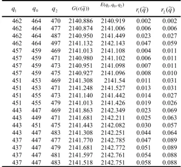
Table IV

For the case

0 ≺

q

₁

≺

q

₀

≤

467 ≺

q

₂

1

q

q₀

2

q

G(c(~q)) E(q1,q0,q2)

r1(~q) r2(~q) 462 464 470 2140.886 2140.919 0.002 0.002 462 464 477 2140.874 2141.006 0.006 0.006 462 464 487 2140.950 2141.449 0.023 0.027 462 464 497 2141.132 2142.143 0.047 0.059 457 459 469 2141.013 2141.108 0.004 0.011 457 459 471 2140.980 2141.102 0.006 0.011 457 459 473 2140.951 2141.098 0.007 0.011 457 459 475 2140.927 2141.096 0.008 0.010 451 453 469 2141.308 2141.54 0.011 0.031 451 453 471 2141.248 2141.527 0.013 0.031 451 455 473 2141.140 2141.442 0.014 0.027 451 455 479 2141.013 2141.426 0.019 0.026 443 447 469 2141.863 2142.349 0.023 0.069 443 449 471 2141.681 2142.211 0.025 0.063 443 451 475 2141.443 2142.082 0.030 0.057 443 447 483 2141.308 2142.251 0.044 0.064 437 447 477 2141.770 2142.785 0.047 0.089 437 447 479 2141.681 2142.772 0.051 0.089 437 447 481 2141.597 2142.761 0.054 0.088 437 447 483 2141.518 2142.751 0.058 0.088

Table V

For the case

0 ≺

q

1

≺

q

0

≺

q

2

≤

467

1

q

q₀

2

q

G(c(~q)) E(q1,q0,q2)

r1(~q) )

~ ( 2 q

r

462 464 466 2140.917 2140.927 0.000 0.003 459 461 465 2141.013 2141.036 0.001 0.008 456 460 462 2141.165 2141.19 0.001 0.015 454 460 462 2141.219 2141.265 0.002 0.018 453 457 463 2141.308 2141.373 0.003 0.023 452 456 458 2141.557 2141.582 0.001 0.033 451 457 463 2141.373 2141.468 0.004 0.028 450 458 464 2141.34 2141.471 0.006 0.028 450 454 460 2141.639 2141.705 0.003 0.039 450 454 458 2141.725 2141.768 0.002 0.042 449 453 461 2141.681 2141.778 0.005 0.042 449 451 459 2141.863 2141.937 0.003 0.050 447 455 463 2141.597 2141.767 0.008 0.042 447 453 461 2141.77 2141.901 0.006 0.048 445 455 463 2141.681 2141.901 0.010 0.048 445 455 459 2141.863 2142.008 0.007 0.053 444 452 460 2142.013 2142.186 0.008 0.061 444 450 458 2142.228 2142.362 0.006 0.070 443 453 461 2141.962 2142.184 0.010 0.061 441 451 459 2142.285 2142.51 0.010 0.077

(6)

V. CONCLUSIONS AND FUTURE RESEARCHES A. Forq~=(q₁,q₀,q₂), compare E(q1,q0,q2)with ))

~ ( (c q

G .

Let q₂−q₀ =Δ₂₀( 0),q₀−q₁ =Δ₀₁( 0)

After computing r1(q~) for different quantity of q1,q0,q2

in tables II-V, we see that when

Δ

₂₀

,

Δ

₀₁ are small, )

, , (q₁ q₀ q₂

E are close toG(c(q~)) and when

Δ

₂₀

,

Δ

₀₁are larger, E(q₁,q₀,q₂)are away fromG(c(q~)).

B. Comparison of the estimate of the total cost in the fuzzy sense

E

(

q

1

,

q

0

,

q

2

)

with the crisp minimal total cost

G

(

q

_*

)

.

From tables II-V and with considering ₍~₎ 2 q

r , we see that

the estimate of the total cost in the fuzzy sense is larger than the crisp minimal total cost G(q_*) and when

Δ

₂₀

,

Δ

₀₁ become larger, E(q₁,q₀,q₂)are away from

G

(

q

_*

)

.

Equation (1) is obtained by assuming the lead times are fixed, and then get the minimal total costG(q_*). But in the reality, usually the time from the ordering point to the delivering point are not fixed and will vary a little. Therefore, we should not use the crisp minimal total costG(q_*), in stead, we should consider the fuzzy case to suit the real situation.

C. Comparison of our article with Mahata et al.’ article

We compare

E

(

q

₁

,

q

₀

,

q

₂

)

of our article with

E

(

q

₁

,

q

₀

,

q

₂

)

of Mahata’ article and we see that the estimate of the total cost in the fuzzy sense in our article is smaller than Mahata’ article.

With this comparison, we conclude that, in fuzzy inventory models, like crisp inventory models, the total cost in models with backorder is smaller than the models without shortage. For the future research, we can solve this model with numerical methods and/or genetic algorithm and get the optimal quantity for the fuzzy total cost.

REFRENCES

[1] S. K. Goyal, "An integrated inventory model for a single supplier single customer problem", International journal of production research 15, 107-111, 1976.

[2] A. Banerjee, "A joint economic lot size model for purchaser and vendor", Decision sciences 17(3), 292-311, 1986. [3] S. K. Goyal, "A joint economic lot size model for purchaser

and vendor:A comment", Decision sciences 19, 236-241, 1988.

[4] L. Lu, "A one vendor multiple buyer integrated inventory model", European journal of operational research 81, 209-210, 1995.

[5] S. K. Goyal, "A one vendor multiple buyer integrated inventory model:A comment", European journal of operational research 82, 209-210, 1995.

[6] L. A. Zadeh, "Fuzzy sets", Information and control 8, 338-353, 1965.

[7] G. Sommer, "Fuzzy inventory scheduling", In Applied Systems and Cybernetics, Volume VI, Edited by G.E.Lasker, pp. 3052 3060, New York, 1981.

[8] K. S. Park, "Fuzzy set theoretic interpretation of economic order quantity", IEEE Transaction on systems,man and cybernetics 17, 1082-1084, 1987.

[9] J. S. Yao, H. M. Lee, "Fuzzy inventory with backorder for fuzzy order quantity", Information Sciences 9, 283-319, 1996. [10] J. S. Yao, H. M. Lee, "Fuzzy inventory with or without

backorder for order quantity with trapezoidal fuzzy number", Fuzzy Sets and Systems 105, 311-337, 1999.

[11] S. C. Chang, J. S. Yao, H. M. Lee, "Economic reorder point for fuzzy backorder quantity", European Journal Of Operation Research 109, 183-202, 1998.

[12] K. Wu, J. S. Yao, "Fuzzy inventory with backorder for fuzzy order quantity and fuzzy shortage quantity", European journal of operational research 150, 320-352, 2003.