Life-cycle earnings role of labor market sorting and job mobility

(1)

A Work Project, presented as part of the requirements for the Award of a Master Degree in Economics from the NOVA - School of Business and Economics.

Life-Cycle Earnings

Role of Labor Market Sorting and Job Mobility

Vicente Sousa Machado de Carvalho e Costa Student N 4199

A Project carried out for the Master in Economics Program, under the supervision of: Professor Pedro Portugal

(2)

Abstract

This paper studies how the underlying factors that determine an individual’s wage changes over their life-cycle, how these factors change at different education levels, and when a worker makes job-to-job moves. Using a longitudinal matched employer-employee data set from the Portuguese Ministry of Labor; I find that human capital accumulation and job mobility play an important role in wage growth during the beginning of an individual’s career. More specifically, I find that after 20 years of work wages increase, on average 41%. A large fraction of the returns to labor market experience is rooted in the returns to general training (25%) but sorting into better paying firms and job/titles is responsible for a significant 19% and 10% of the returns to labor market experience, respectively. Job-to-job mobility also enhances life-cycle earning (14%), as does the ability of the worker (32%).

Keywords: labor market experience, fixed effects, wages, Portugal

1 Introduction

The labor market is one of the most complex but fundamental parts of our economy. As such, a great deal of literature has gone into grasping a better understanding of its mechanisms. At the heart of the field, lies the transaction of a worker’s time for monetary gain, a wage. It is well established that firms pay differing wages to different workers. One of the prevailing explanations is that experience accrued as a worker spends time in the labor market has a large role to play in the matter.

The present study intends to shed some light on the question: ”how the factors that go into determining a worker’s wage change over their life-cycle?”. I am interested in looking into how the underlying factors that determine an individual’s wage change over their life-cycle, at distinct education levels, and when a worker makes job-to-job moves (meaning the worker has no unemployment spells between jobs). These added dimensions will give us a richer insight into the role that these factors play over the life-cycle.

In order to gain the most accurate possible picture of the inner workings of the mech-anisms at work, I intend to apply an approach that has yet to be used in the study of life-cycle wages. This consists of implementing three-way high-dimension fixed effects (an extension of the fixed effects from Abowd et al. (1999)) and a decomposition proposed by Gelbach (2016), producing an unambiguous allocation of wages into its worker, firm, and job-title components. This approach will be applied on a dataset from the Portuguese

(3)

Ministry of Labor, a rich longitudinal matched employer-employee data set, enabling me to adequately tackle the question at hand.

In the Portuguese labor market, on average, the return on experience is 34.5 log points for 20 years of labor market experience (or simply experience), which is equal to a 41% increase1_{. I break down this return into the contributions of firm sorting; job sorting;}

worker’s traits; and human capital, which encompasses on-the-job training. My results also show that as an individual gains experience the main driving force that increases their wage in the first five years of their career is the knowledge they are gaining on-the-job. However, I also show that this effect attenuates significantly after a relatively short period of time. Furthermore, I show that a large part of the returns to experience are accrued in the beginning of an individuals working life. On the education front, my results indicate that the most educated workers have consistently higher returns than the rest. However, if we look at less educated individuals, we can observe that individuals with less than or equal to 4 years of schooling receive higher returns to experience than those with less than or equal to 12 years. Furthermore, I find that the differentiation of the education levels happens before the tenth year of labor market experience, and the benefits of higher levels of schooling is mainly felt early on in the career. With regards to job-to-job mobility, I show that after the third job, the effect of job mobility declines, becoming somewhat constant, meaning that returns to job mobility drop to almost zero. The thesis continues as follows. The following section discusses some of the theoretical foundations that are in the field and relevant existing literature. Sections 3 and 4 go into the model, methodologies and the respective data used. Section 5 presents and discusses the results, and section 6 concludes and suggests further research.

2 Life-Cycle Wages

In this section we will quickly skim over some of the reasons why workers’ wages differ over time, in particular: sorting, job shopping, job matching, human capital accumulation, aggregate effects, and peer effects.

(4)

Beginning with sorting, which entails either the worker or the firm trying to find the best possible employer-employee match, according to their respective expectations. An example in which this may affect the worker’s lifetime wages comes from the fact that whenever an employee quits and is replaced, the firm incurs training, processing, and other turnover costs. As such, the firm wishes to hire applicant with a low propensity to quit. Salop and Salop (1976) outline a way in which a firm may discourage high turnover individuals from applying and encourages low turnover workers to apply for employment. They suggest a firm predictably increase an employees wage with their tenure at the firm. Salop and Salop (1976) argue that, in essence, this causes the applicant to guarantee their longevity with the firm, since they themselves pay the consequences, in terms of foregone higher earnings, if they quit prematurely. In other words, the guarantee enables the firm to trust the applicants protestations that they are a steady and stable worker, at the same time that it makes the firm relatively indifferent to the truth, since the firm no longer bears the onus of being wrong. An employer might find an under-pay-now, over-pay-later compensation plan attractive because of the type of workers likely to sort themselves into their applicant pool.2

Moving on to human capital accumulation. We observe that more productive workers will fetch a higher wage. However, how workers become more productive is a more inter-esting question in and of itself. There are two main ways in which a worker can increase their own productivity through learning. The first is through conventional education, the second is through on-the-job training (itself subdivided into general and job-specific knowledge).2

Topel (1991) offers us two explanations as to how tenure affects wage. His first ex-planation is that productivity rise with seniority, while the other is that tenure merely acts as a proxy for the quality of the job. In contrast, Altonji and Shakotko (1987) pose that if there is growth of quality of jobs because of better matches across time, then this growth causes a downward bias in the estimated returns to tenure. Altonji and Williams (2005) provide a revision of the theory and re-estimate the returns to job seniority. They

(5)

estimate the effect to be 10 years of tenure to be 11 log points. Buchinsky et al. (2010) come to the conclusion that as seniority increases, the cumulative return for the least educated rises by more than for the highly educated. This is because for the less educated individuals who stay in their job, and hence accumulate higher seniority, the main source of human capital is job specific.

On-the-job training can occur through learning by doing, formal training programs at or away from the workplace, or by informally working under the tutelage of a more experienced worker (which we will see later). From the perspective of workers, training depresses wages during the learning period but allows them to rise with enhanced produc-tivity afterward. Thus, workers who opt for jobs that require a training investment are willing to accept lower wages in the short run to get higher pay later on. As with other human capital investments, returns are generally larger when the post-investment period is longer, so we would expect workers’ investments in on-the-job training to be greatest at younger ages and to fall gradually as they grow older.2 _{Bartel and Borjas (1981) show}

that if the worker chooses to invest in on-the-job training, his or her future earnings po-tential can be enhanced. Workers become less willing to invest in human capital as they age and, as such, the yearly increases in potential earnings become smaller and smaller. The acquisition of on-the-job training allows more complex tasks to be performed, or the upward filtering of talented workers as firms discover and promote their ablest workers.

There is a case to be made that ability plays a key role in human capital accumulation, and shapes wages over the life-cycle. Ability to learn rapidly shortens the training period, and fast learners probably also experience lower psychic costs (lower levels of frustration) during training. Thus, people who have the ability to learn quickly are those most likely to seek out and be presented by employers with training opportunities. However, these fast learners are most likely the people who, because of their abilities, were best able to reap benefits from formal schooling. The tendency of better-educated workers to invest more in on-the-job training explains why their age/earnings profiles start low, rise quickly, and keep rising after the profiles of their less-educated counterparts have leveled off. Their earnings rise more quickly because they are investing more heavily in job training, and

(6)

they rise for a longer time for the same reason. In other words, people with the ability to learn quickly select the ultimately high-paying jobs where much learning is required and thus put their abilities to greatest advantage.

As mentioned above, a worker can gain human capital through their peers. Contact between workers enables an environment that fosters the exchange of ideas and learning by doing. This idea sharing is one of the spillovers of education as less educated workers learn from the more educated ones. We see this as, for example, college graduates bring in new knowledge which can benefit other workers (Rauch (1993) was one of the first to empirically study the existence of spillover effects in education). As a worker spends more time in the labor market, there will be more opportunity for them to come into contact with a larger number of more knowledgeable coworkers, and thus gain more from this spillover effect.

Job shopping refers to the search for a suitable job when workers cannot perfectly predict either their performance in (or their liking for) a particular job. From the worker’s point of view, these gaps in their own skill causes an inability to predict job returns -both generally across all jobs, or specific to a particular job. Such theories typically assume that the characteristics of potential offers can be ascertained by the worker by searching (or search good), while Johnson (1978) assumes that some characteristics cannot be known without actual employment experience (or experience good). There exists an educational component important to job shopping, namely the function of education in giving workers information about their abilities. It is plausible to assume that education acts, much like a first job, to narrow the uncertainty a worker feels about their own abilities, which in turn should reduce the role of learning about abilities on-the-job. As such job shopping helps workers find the job in which they will be most productive and have the greatest chance of earning higher wages throughout their lives. Jovanovic (1979) builds a model exploiting this argument. Furthermore, the model also predicts that each workers separation probability is a decreasing function of his job tenure. This is because a mismatch between a worker and his employer is likely to be detected early on rather than late.

(7)

Job search also plays a role in shaping a worker’s wage over their lifetime, as such we will take a closer look into how it does this. Christensen et al. (2005) explain that since job openings occur more or less randomly over time, during any one period in which a worker is on the market, not all potentially attractive openings exist. As time passes, however, jobs open up and workers have a chance to decide whether to apply. Those who have spent more time in the labor market have had more chances to acquire better offers and thus improve upon their initial job matches.

The costs of on-the-job search offers one explanation why we observe that, in general, workers’ wages improve the longer they are active in the labor market. Workers can be viewed as wanting to obtain the best match possible but finding that there is a cost to getting better matches (Shimer and Smith (2000)). Those who see their jobs as a poor match have more incentives to search for other offers than do workers who are lucky enough to already have good matches (high wages). Over time, as the unlucky workers have more opportunity to acquire offers, matches for them should improve. Burdett (1978) puts it succinctly: Older workers in the present study receive higher wage rates, on average, because they have obtained more job offers. And the more job offers a worker receives, the greater the probability a ‘high’ wage rate job will be found.

With all this being said, Lagakos et al. (2018) argue that frictions in the match making process greatly affect the plausibility of some of these theories. If frictions to search and matching lower the incentives or ability of workers to shop for jobs, they are less likely to climb the job ladder and will forgo some of the potential increase in labor productivity over the life cycle. Alternatively, long-lasting frictions may prevent workers from sorting to the jobs that are most suitable to their heterogeneous skills and tastes. Again, the implication would be that workers forgo labor productivity increases as they age.

From some of the already mentioned works, we can see the impact of job mobility on wages. Buchinsky et al. (2010) conclude that the timing of a move in a career matters. Early moves being most beneficial to college educated workers whereas late moves can be very detrimental for workers with lower education. Short spells can sometimes be good, and other times be bad. Mobility through the wage distribution is achieved through

(8)

a combination of wage increases within the firm and across firms. The former is more important for wage growth of high school dropouts because of their lower returns to experience. The latter is more important for college graduates, because both returns to experience and seniority are quite large. Later, Boroviˇckov´a and Shimer (2017) find that the correlation between a worker’s type and their employer’s type is quite high, lying between 0.4 and 0.5 and is reasonably stable over time. One interpretation of the results is that workers gradually sort over the life cycle. At the start of their careers, there is a lot of uncertainty about a workers’ type and so sorting is imperfect. As the worker grows older, the market learns the worker’s type and the best workers sort into the best jobs.

We will now turn to the aggregate effects that change a worker’s wage over their life-cycle. Over a worker’s lifetime there is an advancement in technology this effect is even more accentuated in the last century- making tasks easier and workers more productive. Although this is true across the entire labor market, we can argue that the worker is more productive than a younger version of themselves, and as such will fetch a higher wage.

I will rely in the works of Altonji et al. (2013) as a starting point. Their main results are: first, they conclude that job changes are induced by high outside offers and deterred by the job-specific wage component of the current job, which is consistent with job search theory. Second, wages are highly persistent. This persistence is the combination of the effects of both observed and unobserved heterogeneity, the job-specific wage component, which depends positively on offers in previous jobs, and strong persistence in representing the value of the worker’s general skills. Third, the variance and mean of earnings changes are greatly affected by shocks leading to job changes. Finally, that job-shopping, the accumulation of tenure, and the growth in general skills account for log point wage in-creases of 13, 11, and 61, respectively, over the first 30 years in the labor market. Finally, they find that job mobility plays a key role in the variance of career earnings. Variables determined by the first year of employment, including unobserved heterogeneity, educa-tion, and initial draws of the general skill and job-specific wage components, collectively account for 44.6% of lifetime wages.

(9)

the variation in the prices of goods is due to factors other than marginal cost, the notion that wages differ substantially among equally skilled workers remains highly controversial.

3 Empirical Methodology

A big focus in labor economics is what determines wages, and a large amount of the literature in this subject has focused on the relationship between education and wages. Economists such as Mincer defend a human capital theory of education, in which they argue education raises productivity. Mincer (1974) argues that there are more types of investment in human capital, other than schooling, although schooling is an important stage in the life-cycle of self-investment. Mincer states that we must take into account pre-school (home) and post-pre-school (job) investments in addition to pre-schooling, when we think of the life-cycle stages, or ways in which human capital is built up. The Mincer model was first derived to capture the schooling rate of return on earnings (Mincer (1958)), where individuals decided the education level that maximized the present value of their lifetime earnings. Mincer argues that there are more types of investment in human capital, other than schooling, one such example is vocational training (labor market experience). As such, Mincer added the impact on earnings of investments in human capital throughout working life. Suggesting that the proportion of earnings given to investment in human capital decreases linearly with labor market experience, the base specification is given by:

wit= β0+ β1Sit+ β2LM Xit+ β3LM Xit2 + β4Gi+ εit (1)

where witis the natural logarithm of wage belonging to worker i(i = 1, . . . , N ) in year t(t =

1, . . . , Ti). There are Ti observations for each individual i and a total of N∗ observations.

Sit is the level of schooling for individual i in time t. LM Xitis individual i’s labor market

experience at time t, and Gi is a gender dummy for individual i; εit is an error which

is assumed to be uncorrelated with the covariates. The use of logarithms on earnings is consistent with both the units of investment being in time and not monetary units (Mincer (1975)), and the accurate fit of log-linearity for the major wage distribution of

(10)

Mincers sample. Additionally, it simplifies the interpretation of small coefficients.

Adding more complexity to the model, and as much of the literature, I will use a variation on the additive worker and firm effects wage model proposed by Abowd et al. (1999) also known as AKM, as it has become the benchmark for analysis in matched (or linked) employer-employee data. In their seminal study of the French labor market, Abowd et al. (1999) specified a model for log wages that includes additive fixed effects for workers and firms. Specifically, their model for the log wage of person i in year t takes the form:

wit = Xitβ + θi+ φF (i,t)+ εit (2)

where Xit summarizes the time-varying regressors (quadratic on labor market experience,

tenure and log of firm size), θi is the person effect capturing the (time-invariant) portable

component of earnings ability, β is a vector of coefficients for the observed characteristics of the same individual, and φF (i,t) is the firm effect for the firm in which individual i

is working in at time t (denoted by the function F (i, t) = 1, . . . , F ). Each of the fixed effects captures observed and unobserved individual time-invariant heterogeneity. The innovation in the AKM framework is the presence of the firm effects, which allows for the possibility that some firms pay systematically higher or lower wages than other firms. 3

Expanding on the model I have seen so far, I follow Torres et al. (2018) and allow a flexible specification for the effect of labor market experience, and also add to the AKM model a job-title fixed effect. Job-title effects reflect the distinct set of occupational tasks performed by workers that serve to define occupational boundaries. Their model is as follows:

wit = Xitβ + θi+ φF (i,t)+ λJ (i,t) + ξE(i,t)+ δt+ εit (3)

3_{Another, more technical issue that arises with the AKM model is appropriate specification of the}

effects of age. Following Mincer (1974), it is conventional to include a polynomial in age or potential experience in Xit. However, it is also standard to include a set of year indicators in Xit (for example,

to adjust for changing macroeconomic conditions). This raises an identification problem because age can be computed as calendar year minus birth year. Hence, I face the problem of distinguishing additive age, year, and cohort effects, where cohort effects are understood to load into the person effects. While the firm effects are invariant to how age and time effects are normalized, different normalizations will yield different values of the person effects and the covariate index. An approach to dealing with this problem is to impose a linear restriction on the effects of age or time. Card et al. (2018) suggest substituting age and age2with (age − 40)2. The way in which I intend to get around this issue is to forgo calculating the effects of age on wage, but keying into the effects of labor market experience on wage.

(11)

where I add new variables to equation (2), the first of which is λJ (i,t), this is the job-title

fixed effect for job-title in which individual i occupies at time t (denoted by the function J (i, t) = 1, . . . , J ). ξE(i,t) is the labor market experience fixed effect for each year of labor

market experience individual i has at time t (denoted by the function E(i, t) = 1, . . . , E). Another new addition is δt, which is a calendar year fixed effects included to capture the

macroeconomic environment (business cycle). In summary, there are seven components that explain the wage variability:

1. the workers’ permanent heterogeneity or worker quality, θi;

2. the firms’ permanent heterogeneity or firm sorting, φF (i,t);

3. the job-titles’ permanent heterogeneity or job-title sorting, λJ (i,t);

4. the calendar years’ permanent heterogeneity or calendar year fixed effects, δt;

5. on-the-job training or human capital accumulation, ξE(i,t);

6. the time-varying characteristics, Xitβ (tenure, tenure squared, and log of firm size);

7. an error term component (εit), assumed to follow the conventional assumptions.

I am interested in using these estimates to see how they change over a worker’s life-cycle, as such I must restrict the data set to connected observations for which compara-bility of the estimates of the fixed effects is assured. To do this I will use the algorithm of Weeks and Williams (1964) to identify connected observations. This algorithm identifies a subset of the data in which all workers’ fixed effects are connected. If I restrict analysis to this subset of the data, I assure that the estimates of the fixed effects are comparable. Once I have the model I wish to estimate, in this case equation (3), I must then employ an adequate method for estimation. Abowd et al. (1999) proposed a solution that yielded an approximation to the full least squares solution of a linear regression model with two high-dimensional fixed effects, however, this method would not be optimal as it involves the inversion of a huge matrix. Making it impossible to achieve using standard software routines and present-day computers. In a later paper, Abowd et al. (2002) presented a conjugate gradient algorithm that led to the exact least squares solution, however, they estimate models with only two fixed effects. More recently, Guimar˜aes and Portugal (2010) demonstrated that it is possible to obtain the exact least squares

(12)

solution for linear regression models with two or more high-dimensional fixed effects with a methodology that is based on a partitioned algorithm strategy and follows an iterative procedure that leads to the exact solution of the least squares problem. This approach is computationally intensive but imposes minimum memory requirements (as opposed to the heavy memory constraints imposed in the solution given by Abowd et al. (2002)). As such, I will use the iterative algorithm proposed by Guimar˜aes and Portugal (2010).4

Now, using equation (3) and the iterative algorithm I must show how each fixed effect contributes to wages over a worker’s life-cycle. To this end I will use a similar approach to Cardoso et al. (2016) (in this paper the authors study the gender pay gap) and Addison et al. (2018) (in this paper the authors study the union wage gap). In order to disentangle the contributions of the fixed effects to the passage of time, I will use the decomposition first suggested by Gelbach (2016) (like Cardoso et al. (2016)). Based on the formula for omitted variable bias, Gelbach’s decomposition allows us to us to disentangle the contribution of each excluded variable (each fixed effect) to the variation of the coefficient estimate(s) of the labor market experience variable(s). This then quantifies the impact of each of the fixed effects on the relationship between wages and labor market experience5. In practice, the decomposition is achieved by estimating regressions in which the fixed effects become the dependent variables and the regressors are those of equation (3). Then I can provide a graphical representation of how these fixed effects affect the return to experience.

4 Data

I will be using a longitudinal matched employer-employee data set for Portugal, known as the Quadros de Pessoal for the years 1986 to 2009 (excepting 1990 and 2001) and from its successor survey the Relatrio ´Unico for the years 2010 to 2013. This unique dataset is

4_{To achieve this I will be using the STATA command ”reghdfe” written by Correia (2016)}

5_{The way in which I define labor market experience at time t is as a sum of all the accumulated tenure}

a worker has accrued up to time t - in practice this is the sum of tenure of all past and current jobs of said worker. As a worker ages, their labor market experience will increase accordingly, if they don’t suffer spells of unemployment. Since I am using labor market experience instead of age, what is meant behind life-cycle wages is how wages change as a worker gains more experience.

(13)

administered by the Portuguese Ministry of Labor, and is taken from a mandatory annual survey 6 of all firms with at least one wage earner in the reference month - March of each year until 1993, October thereafter. However, civil servants, self-employed, and household employees are not covered. Furthermore, since the share of wage-earners in agriculture is low, the coverage of this sector is low. Nonetheless, for manufacturing and the services private sector of the economy, the survey covers virtually the entire population of workers and firms. Due to the mandatory nature of the survey, problems commonly associated with panel data sets, such as panel attrition, are considerably attenuated.

Turning to specifics, the data set includes the following information on each worker: social security identifier, gender, age, level of education, occupation, employment status, tenure, monthly earnings, normal and overtime hours, time elapsed since last promotion, and the worker’s job-title (so-called professional category or categoria profissional ). The schooling information refers to the highest completed level of education.7 _{The information}

on earnings includes the base wage (gross pay for normal hours of work), regular benefits, and overtime pay. The data set also includes the following information on the firms: firm identifier, location, industry, legal form, ownership, year of formation, sales, and capital. After some cleaning of the data (which included, removing entries with no social se-curity number, and missing wages), I applied some restrictions to the data set. I began by restricting the analysis to full-time (more than 120 monthly hours) workers with ages between 25 and 54, in hopes to eliminate any selection bias into or out or the work-force (as per Bingley and Cappellari (2018)). I dropped from the analysis workers whose monthly wages were below 75% of the mandatory minimum wage (which corresponds to the minimum wage for apprentices). I further dropped any worker with an experience that suggested they began employment with the age lower than 15. As mentioned in section 4, we must restrict the data to a subset of the data in which all workers’ fixed effects are connected. This largest connected set comprises 5,994,065 unique worker entries and

6_{Each year, around 300 different collective agreements are negotiated. The collective agreement defines}

wage floors for each particular job-title (so-called professional category or categoria profissional ). The main reason why this survey was created was, indeed, to allow the officials from the Ministry of Labor to verify whether the employers were complying with the wage floors established by the collective agreement for the job-title of the worker.

(14)

678,258 unique firm entries, for a total of 38,549,942 observations.

5 Empirical Results

I will be analyzing the results in three section. The first will encompass an overarching view of how wages change as a worker gains experience, on average. The second will provide an educational breakdown of how wages change through the life-cycle. In both of the previous cases, I will use dummy variables for each year of experience in order to analyze to intended mechanisms. The third and final section will look at job changes, and how they affect the factors that go into determining wage. During each of the different breakdowns we must keep in mind that we are dealing with changes in log points of real hourly wage.

5.1 Breakdown of Entire Population

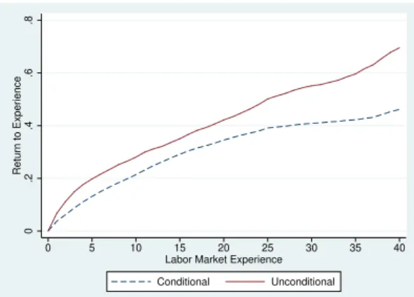
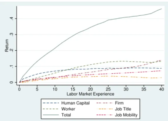
I will start off with the analysis of the population on a broader scale. Figure 1 shows both how wages change as a worker gains experience (Figure 1a), which we can equate to the returns to experience, and the decomposition of said returns(Figure 1b).

0 .2 .4 .6 .8 Return to Experience 0 5 10 15 20 25 30 35 40 Labor Market Experience

Conditional Unconditional 0 .1 .2 .3 .4 Return 0 5 10 15 20 25 30 35 40 Labor Market Experience

Human Capital Firm Worker Job Title Total

(a) Returns to Experience. Both curves are normal-ized to zero. Unconditional, regression of experience on log wages, not controlling for any other factors. Conditional, regression of log wages, controlling for tenure, tenure squared, firm size, gender, education, and calendar year fixed effects (Regression I of Ap-pendix III)

(b) Decomposition of Returns to experience. Gelbach decomposition of the Conditional curve of (a). Curves normalized to zero. Showing firm, job-title, worker, and experience contributions to returns of experience (Regression II of Appendix III)

Source: Quadros de Pessoal

Figure 1: Graph of Returns to Experience and its Decomposition

(15)

regression of wage on experience, and a conditional curve which represents the regression of wage on experience with the added controls of specification (I)8 where I have controlled for education, gender, and the calendar year. This conditional curve of figure 1a is the same as the Total curve in figure 1b. As 23 years is the 90th percentile for experience, I will mostly discuss the values at 20 years of experience. From Figure 1a it can be seen that the return on experience is 34.5 log points (a two fifth increase) for 20 years of experience.9

We can decompose this 34.5 log point return on experience into the respective con-tributions from the firm sorting, worker quality, job-title sorting, and human capital accumulation. Here, it is to our benefit to understand that the returns to experience of, say firm sorting represents the log point increase in real hourly wage that would occur if individuals were equally paid across firms regardless of experience, conditional on all other variables included in the full model.10 _{We can see that firm sorting accounts for 6.6}

log points (approximately one fifth of the return to experience); job-title sorting accounts for 3.6 log points (approximately one tenth of the return to experience); worker quality accounts for 12.1 log points (approximately one third of the return to experience); and, what I am attributing to human capital, which encompasses on-the-job training, accounts for 12.2 log points (approximately one third of the return to experience).

We can observe from Figure 1a that the returns to experience do not increase in a linear fashion. In the first five years of experience an individual has a return to experience of 19.8 log points. In contrast, in the 5 years leading up to the 20th _{year of experience}

the return is 7.1 log points. This indicates that a large part of the returns to experience are accrued in the beginning of an individuals working life. To better understand where these different gains come from we must turn to Figure 1b. In the first five years of experience the model shows that an individual gains 13.1 log points; approximately half of the return to experience comes from human capital accumulation; one sixth of the return to experience comes from the firm sorting; one tenth of the return to experience

8 _{The model specifications can be seen in the Appendix III.}

9_{This comes as a result of calculating the difference of wages at 20 years of experience with that of 0}

years

(16)

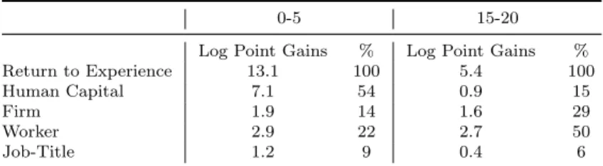
comes from the job-title sorting; and one fifth of the return to experience comes from the worker quality. In the 5 years leading up to the 20th year of experience the model shows that an individual gains 5.4 log points; approximately one sixth of the return to experience comes from human capital accumulation; one third of the return to experience comes from the firm sorting; one tenth of the return to experience comes from the job-title sorting; and half of the return to experience comes from the worker quality. These values are summarized in the following table.

0-5 15-20

Log Point Gains % Log Point Gains %

Return to Experience 13.1 100 5.4 100

Human Capital 7.1 54 0.9 15

Firm 1.9 14 1.6 29

Worker 2.9 22 2.7 50

Job-Title 1.2 9 0.4 6

Note: 0-5 columns show how the returns to experience and its components evolve as a worker gains 5 years of experience, starting with 0 years. 15-20 columns show how the returns to experience and its components evolve as a worker gains 5 years of experience, starting with 15 years. Log point gains column is calculated as the difference of the values of each fixed effect of end of period and beginning of period. % column shows the respective percentage of each fixed effect with regards to the return on experience. Source: Quadros de Pessoal

Table 1: Return on Experience for different time frames

What these results show is that as an individual gains experience the main driving force that increases their wage in the first five years of their career is the knowledge they are gaining on-the-job. This is supported by the theory of human capital accumulation presented in section 3. However, I also show that this effect drops significantly after a relatively short period of time (just from the first to the second year, the yearly contribu-tion to the returns to experience shrink from three quarters to half). This goes to suggest that most of the benefits of on-the-job learning is reaped early in an individual’s career. Which makes sense, since more often than not, an individual starts a job with little to no knowledge of the trade and as such increases their impact considerably in the first year of the job. Furthermore, it makes sense to invest in human capital at the beginning of ones working life, as this allows a larger return on investment. It is interesting to note how the firm sorting varies in these two time frames. This increase in contribution could be representative of some of the compensation plans employed by firms.

(17)

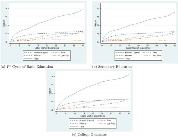
5.2 Breakdown by Education

I will limit the focus to only a few education levels. As we can see from the descriptive statistics the two levels of education with the highest shares are: 1st _{cycle of basic}

edu-cation, 2nd _{cycle of basic education, and secondary education, respectively. Additionally,}

it is interesting to observe college graduates, as it pertains to the most educated segment of the population. Since 1st cycle of basic education and 2nd cycle of basic education only differ in two extra years of education, I will focus on the less educated group. Due to these facts, I will focus a greater part of the analysis to these three levels of education. 11

0 .1 .2 .3 .4 Return 0 5 10 15 20 25 30 35 40 Labor Market Experience

Human Capital Firm Worker Job Title Total 0 .1 .2 .3 .4 Return 0 5 10 15 20 25 30 35 40 Labor Market Experience

(a) 1st_{Cycle of Basic Education} _{(b) Secondary Education}

0 .1 .2 .3 .4 Return 0 5 10 15 20 25 30 35 40 Labor Market Experience

(c) College Graduates

Note: Each figure shows the decomposition of returns to labor market experience for different levels of education. Curves normalized to zero. Showing firm, job-title, worker, and human capital contributions to the returns to experience (Regression IV of Appendix III)

Figure 2: Decomposition of Returns to Experience by Education Levels

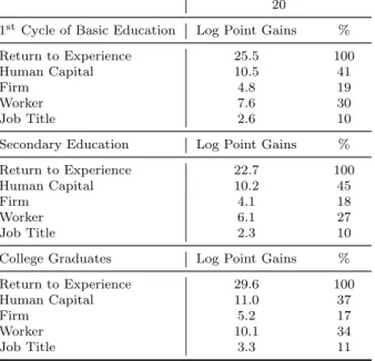
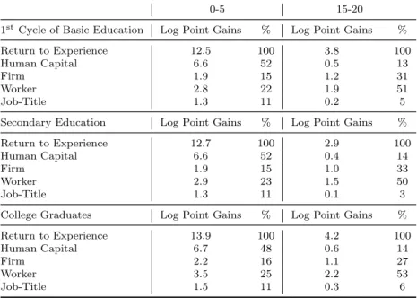
The interpretation of the results is similar to that shown in the section above. I will begin by presenting the return to experience of each level of education at 20 years of experience, and its respective breakdown, shown in the following table:

(18)

20

1stCycle of Basic Education Log Point Gains %

Return to Experience 25.5 100

Human Capital 10.5 41

Firm 4.8 19

Worker 7.6 30

Job Title 2.6 10

Secondary Education Log Point Gains %

Firm 4.1 18

Worker 6.1 27

Job Title 2.3 10

College Graduates Log Point Gains %

Firm 5.2 17

Worker 10.1 34

Job Title 3.3 11

Note: Log point gains column corresponds to the values of the returns to experience and its components at 20 years of experience. % column shows the respective percentage of each component with regards to the return on experience. Source: Quadros de Pessoal

Table 2: Decomposition of Returns by Education Levels at 20 years of Experience

From this we see that college graduates have consistently higher returns than the rest, suggesting that there is some merit to the theory of how ability plays a role on wages (see section 3). We also see that at the 20-year mark, the percentage contributions of the different components do not change much with respect to education levels, human capital accounts for two fifths to half of the return to experience, the firm effect accounts for one fifth of the return to experience, the job-title sorting accounts for a tenth of the return to experience, and the worker quality varies between a fourth and a third of the return to experience. This would suggest that workers of different levels of education gain from the same sources at relatively the same experiences. This will be something that we will analyze further when we observe the curve as a whole.

The following table summarizes the relevant values for the curve at the various edu-cation levels, similarly to the section above.

On a level by level basis the interpretation for the results shown above do not differ much from that of the population as a whole. The results show that as an individual gains experience the main driving force that increases their wage in the first five years of their career is the knowledge they are gaining on-the-job. I also show that this effect

(19)

0-5 15-20

1stCycle of Basic Education Log Point Gains % Log Point Gains %

Firm 1.9 15 1.2 31

Worker 2.8 22 1.9 51

Job-Title 1.3 11 0.2 5

Secondary Education Log Point Gains % Log Point Gains %

Firm 1.9 15 1.0 33

Worker 2.9 23 1.5 50

Job-Title 1.3 11 0.1 3

College Graduates Log Point Gains % Log Point Gains %

Firm 2.2 16 1.1 27

Worker 3.5 25 2.2 53

Job-Title 1.5 11 0.3 6

Note: 0-5 columns show how the returns to experience and its components evolve as a worker gains 5 years of experience, starting with 0 years. 15-20 columns show how the returns to experience and its components evolve as a worker gains 5 years of experience, starting with 15 years. Log point gains column is calculated as the difference of the values of each fixed effect of end of period and beginning of period. % column shows the respective percentage of each fixed effect with regards to the return on experience. Source: Quadros de Pessoal

Table 3: Return on Experience for different time frames by levels of education

drops significantly after a relatively short period of time. This suggests that most of the benefits of on-the-job learning is reaped early in that individual’s career, and through human capital investment. However, we know see that there is a larger decrease in the effect of job-title sorting, on all education levels. This would suggest that the job-title comes to play a larger role as a worker gains experience. This would suggest that as an individual gains experience and climbs the job ladder their wage increases with them.

From the information provided so far, it would seem that workers of differing education levels receive identical returns to experience. This is understandable as we are missing a key piece of information, namely, how the returns fair against one another not being normalized. The following figures will help us understand how the returns to experience change over different education levels.

Figure 3 shows a similar image to figure 1a from the section above. However due to the sheer amount I must separate the uncontrolled and controlled curve into two separate figures (figure 3a and 3b respectively). One of the surprises that we can see from figure 2b is that individuals with 1st _{cycle of basic education have a higher relative return on}

(20)

0 .5 1 1.5 2 Return to Experience 0 5 10 15 20 25 30 35 40 Labor Market Experience

1st Cycle of Basic Education Secondary Education College Graduates 0 .1 .2 .3 .4 Return to Experience 0 5 10 15 20 25 30 35 40 Labor Market Experience

1st Cycle of Basic Education Secondary Education College Graduates

(a) Returns to Experience by different levels of educa-tion. Showing log wages on experience not controlling for any other factor.

(b) Returns to Experience by different levels of educa-tion. Curves normalized to zero. Showing experience on log wages, controlling for tenure, tenure squared, firm size, gender, education, and calendar year fixed effects (Regression III of Appendix III) .

Figure 3: Returns to Experience separated by levels of education

experience than those with higher education (individual with a secondary education). This would suggest that in the Portuguese economy, once we control for factors such as firm, job-title, worker, and calendar fixed effects, individuals with less than or equal to 4 years of schooling receive higher returns to experience than those with less than or equal to 12 years. However, the most educated level (college graduates) receives the highest returns. To clarify, this goes to show that not only do college graduates fair best because they begin their career with higher paying wages, but they also receive higher return on the experience they gain over their life-cycle. As mentioned in section 3, this could be due to the fact that people with the ability to learn quickly select the ultimately high-paying jobs where much learning is required and thus put their abilities to greatest advantage.

Another interesting result that can be seen from figure 2b is the accelerated growth of the returns for college graduates, after which it seems that the growth of all four levels becomes quite similar. after the 10th _{year of experience mark it seems that all four levels}

of education follow parallel growth patterns. This would indicate that the differentiation of the education levels happens before this point, and the benefits of higher levels of schooling is mainly felt early on in the career. From these findings and figure 2a we can conclude that the overall difference between education levels is due to the higher starting salary that individuals from higher education levels attain.

(21)

5.3 Job Change

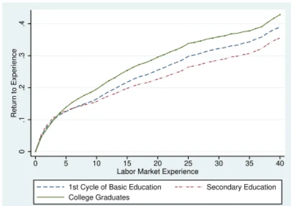
Shifting gears, I will now present how the returns to labor market experience are affected when we take into consideration worker making job-to-job moves. I will only present the findings for individuals with less than 7 jobs, and I define a job as the marriage of one specific individual with a specific firm. Thus, these results will shed some light as to the return of job mobility, and will help us shed light on to the claims made by theories in job shopping, job matching, and sorting.

0

.05

.1

.15

.2

Return on Number of Jobs

1 2 3 4 5 6 Number of Jobs Conditional Unconditional 0 .1 .2 Return 1 2 3 4 5 6 Number of Jobs

Job Mobility Firm Worker Job Title Total

(a) Impact of the Number of Jobs. Both curves nor-malized to zero. Unconditional, regression of number of jobs on log wages, not controlling for any other fac-tors. Conditional, regression of number of jobs on log wages, controlling for tenure, tenure squared, firm size, gender, education, and calendar year fixed effects (Re-gression V of Appendix III)

(b) Decomposition of Returns. Gelbach decomposition of the Conditional curve of (a). Curves normalized to

zero. Showing firm, job-title, and worker

contribu-tions to the impact of number of jobs (Regression VI of Appendix III)

Figure 4: Graph of Impact of the Number of Jobs and its Decomposition

From figure 4a (which has a similar reading as figure 1a) we can see that as an indi-vidual makes job-to-job changes, their impact of the number of jobs increases. From the shape of the overall curve we see that there seems to be some sort of diminishing returns to the number of jobs, as the first job nets about a 6.1 log point increase to hourly wage, while the sixth job nets a 2.4 log point increase to hourly wage. The decomposition of said impact of the number of jobs are shown in figure 4b.

From figure 4b we can see how the impact of the number of jobs is partially driven by firm sorting. The contributions of worker quality and job-title sorting are equal up until the second job, where the job-title sorting seem to follow a linear growth and the worker quality appears to increase substantially. The interpretation of job mobility effects, that is, the impact of the number of jobs after taking sorting into account, suggests that as

(22)

an individual changes job they are entering in a better match, and/or are obtaining a higher salary from their new firm in order to entice the change. As mentioned, after the third job, the effect of job mobility attenuates, becoming somewhat constant, meaning that there returns to job mobility drop to almost zero.

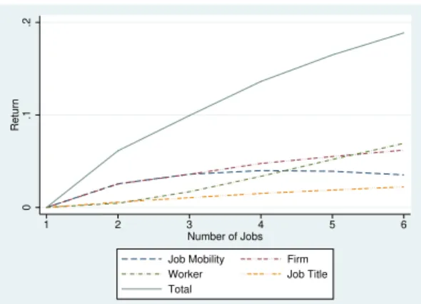
With these result we have a better understanding of how wages change as an individual changes jobs, and what are the driving factors of the wage increases. However, we are lacking information on the role on-the-job training plays when it comes to job mobility. For this we must turn to a different analysis. The following figure is similar to that of figure 1, however, now I am also controlling for the number of jobs. With this added dimension, and comparing both figures 1 and 5, it can be seen what the effect of job mobility have on gains from experience.

0 .2 .4 .6 .8 Log Wage 0 5 10 15 20 25 30 35 40 Labor Market Experience

Conditional Unconditional 0 .1 .2 .3 .4 Return 0 5 10 15 20 25 30 35 40 Labor Market Experience

Human Capital Firm Worker Job Title Total Job Mobility

(a) Returns to Experience. Both curves normalized to zero. Unconditional, regression of log wages on ex-perience, not controlling for any other factors. Con-ditional, regression of log wages on experience, con-trolling for tenure, tenure squared, firm size, gender, education, and calendar year fixed effects (Regression I of Appendix III)

(b) Decomposition of Returns. Gelbach decomposition of the Conditional curve of (a). Curves normalized to zero. Showing firm, job-title, worker, human capital, and number of jobs contributions to the returns to experience (Regression VII of Appendix III)

Figure 5: Graph of Returns to Number of Jobs and Decomposition for whole population

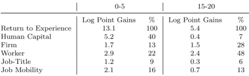
These figures, specifically figure 5b, gives us a richer breakdown of the 34.5 log point return on experience that we found in section 5.1. This is to be expected as I am adding a new variable (previously omitted), job mobility. The main change to the results found in section 5.1 at 20 years of experience is a reduction to 8.5 log point (from 12.2 log points) for human capital, it now accounts for approximately one fourth of the return to experience. the newly added dimension, job mobility accounts for 4.9 log point (approximately one tenth of the return to experience).

(23)

0-5 15-20

Log Point Gains % Log Point Gains %

Return to Experience 13.1 100 5.4 100 Human Capital 5.2 40 0.4 7 Firm 1.7 13 1.5 28 Worker 2.9 22 2.4 48 Job-Title 1.2 9 0.3 6 Job Mobility 2.1 16 0.7 13

Note: 0-5 columns show how the returns to experience evolve and its components as a worker gains 5 years of experience, starting with 0 years. 15-20 columns show how the returns to experience and its components evolve as a worker gains 5 years of experience, starting with 15 years. Log point gains column is calculated as the difference of the values of each fixed effect of end of period and beginning of period. % column shows the respective percentage of each fixed effect with regards to the return on experience. Source: Quadros de Pessoal

Table 4: Return on Experience for different time frames

Comparing table 1 and the table 4 we can see that when adding this new dimension, most of the already calculated returns suffer very minor changes. This cannot be said for the returns of human capital, these reduce significantly, this suggests that there is quite a bit of human capital accumulation that arrives from job changing, which falls in line with some of the theories of human capital accumulation. From the new result we can see that the returns from job mobility stay relatively constant, percentage wise, as an individual gains experience. This would imply that finding a better job match has the same relative benefits for any experience level.

6 Conclusion

I used a combination of high-dimensional fixed effects regression model, the decomposition proposed by Gelbach (2016) on a rich longitudinal matched employer-employee data set from the Portuguese Ministry of Labor, in order to study the underlying factors that determine an individual’s wage change over their life-cycle, how these factors differ at different education levels, and how they differ when a worker makes job-to-job moves.

I find that on average, the return on experience is 34.5 log points for 20 years of experience. I break down this return into: where an individual works; what title an individual holds; the worker’s traits; and human capital, which encompasses on-the-job training. More specifically, I find that after 20 years of work wages increase, on average 41%. A large fraction of the returns to labor market experience is rooted in the returns

(24)

to general training (25%) but sorting into better paying firms and job/titles is responsible for a significant 19% and 10% of the returns to labor market experience, respectively. Job-to-job mobility also enhances life-cycle earning (14%), as does the ability of the worker (32%). My results also show that as an individual gains experience, the main driving force that increases their wage in the first five years of their career is the knowledge they are gaining on-the-job. However, I also show that this effect drops significantly after a relatively short period of time. Furthermore, I show that a large part of the returns to experience are accrued in the beginning of an individuals working life.

On the education front, my results indicate that the most educated workers have consistently higher returns than the rest. However, if we look at less educated individuals, we can observe that individuals with less than or equal to 4 years of schooling receive higher returns to experience than those with less than or equal to 12 years. Furthermore, I find that the differentiation of the education levels happens before the tenth year of labor market experience, and the benefits of higher levels of schooling is mainly felt early on in the career. On job-to-job mobility, I show that after the third job, the effect of job mobility declines, becoming somewhat constant, meaning that there returns to job mobility drop to almost zero.

Further research on life-cycle wages is left open after this result. Firstly, it would be interesting to approach this subject from an age perspective, as opposed to experience. As mentioned earlier this would run into an age-cohort-year problem in the worker fixed effect, but applying a correct specification on age could solve this problem. This was the approach I initially took, but quickly came to the conclusion that I would not be fruitful. Perhaps with greater resources this approach would result in interesting findings. This would be a research which would be interesting to see not only because of its results, but also because it could provide further robustness to the results of this thesis.

Another possible avenue further research could use this study as a starting point would be to flesh out some of the job mobility dimensions presented, I did not include the plethora of complexity that this area requires, and as such am not able to pinpoint the root of the effects of job mobility to one concrete theory (job shopping, job matching

(25)

or sorting). It would be interesting to see the results of such a study to see how it would farther the knowledge of the field. Hopefully, the findings of this thesis will stimulate in other researchers the motivation to carry this research.

7 References

Abowd, John M., Robert H Creecy, Francis Kramarz, et al. (2002). Computing person and firm effects using linked longitudinal employer-employee data. Technical report, Center for Economic Studies, US Census Bureau.

Abowd, John M., Francis Kramarz, and David N Margolis (1999). High wage workers and high wage firms. Econometrica 67 (2), 251–333.

Addison, John T., Pedro Portugal, and Hugo Vilares (2018). The sources of the union wage gap: The role of worker, firm, match, and job-title heterogeneity.

Altonji, Joseph G. and Robert A Shakotko (1987). Do wages rise with job seniority? The Review of Economic Studies 54 (3), 437–459.

Altonji, Joseph G., Anthony A Smith Jr, and Ivan Vidangos (2013). Modeling earnings dynamics. Econometrica 81 (4), 1395–1454.

Altonji, Joseph G. and Nicolas Williams (2005). Do wages rise with job seniority? a reassessment. ILR Review 58 (3), 370–397.

Bartel, Ann P. and George J Borjas (1981). Wage growth and job turnover: An empirical analysis. In Studies in labor markets, pp. 65–90. University of Chicago Press.

Bingley, Paul. and Lorenzo Cappellari (2018). Workers, firms and life-cycle wage dynamics. IZA Discus-sion Paper 11402.

Boroviˇckov´a, Katar´ına. and Robert Shimer (2017). High wage workers work for high wage firms. Technical report, National Bureau of Economic Research.

Buchinsky, Moshe., Denis Fougere, Francis Kramarz, and Rusty Tchernis (2010). Interfirm mobility, wages and the returns to seniority and experience in the united states. The Review of economic studies 77 (3), 972–1001.

Burdett, Kenneth. (1978). A theory of employee job search and quit rates. The American Economic Review , 212–220.

Card, David., Ana Rute Cardoso, J¨org Heining, and Patrick Kline (2018). Firms and labor market inequality: Evidence and some theory. Journal of Labor Economics 36 (S1), S13–S70.

Cardoso, Ana Rute., Paulo Guimar˜aes, and Pedro Portugal (2016). What drives the gender wage gap? a look at the role of firm and job-title heterogeneity. Oxford Economic Papers 68 (2), 506–524.

(26)

Christensen, Bent Jesper., Rasmus Lentz, Dale T Mortensen, George R Neumann, and Axel Werwatz (2005). On-the-job search and the wage distribution. Journal of Labor Economics 23 (1), 31–58. Correia, Sergio. (2016). Linear models with high-dimensional fixed effects: An efficient and feasible

estimator. Technical report. Working Paper.

Ehrenberg, Ronald G., Robert S Smith, et al. (2016). Modern labor economics: Theory and public policy. Routledge.

Gelbach, Jonah B. (2016). When do covariates matter? and which ones, and how much? Journal of Labor Economics 34 (2), 509–543.

Guimar˜aes, Paulo. and Pedro Portugal (2010). A simple feasible procedure to fit models with high-dimensional fixed effects. Stata Journal 10 (4), 628.

Johnson, William R. (1978). A theory of job shopping. The Quarterly Journal of Economics, 261–278. Jovanovic, Boyan. (1979). Job matching and the theory of turnover. Journal of political economy 87 (5,

Part 1), 972–990.

Lagakos, David., Benjamin Moll, Tommaso Porzio, Nancy Qian, and Todd Schoellman (2018). Life cycle wage growth across countries. Journal of Political Economy 126 (2), 797–849.

Mincer, Jacob. (1958). Investment in human capital and personal income distribution. Journal of political economy 66 (4), 281–302.

Mincer, Jacob. (1974). Schooling, experience, and earnings. human behavior & social institutions no. 2. Mincer, Jacob. (1975). Education, experience, and the distribution of earnings and employment: an

overview. In Education, income, and human behavior, pp. 71–94. NBER.

Rauch, James E. (1993). Productivity gains from geographic concentration of human capital: evidence from the cities. Journal of urban economics 34 (3), 380–400.

Salop, Joanne. and Steven Salop (1976). Self-selection and turnover in the labor market. The Quarterly Journal of Economics, 619–627.

Shimer, Robert. and Lones Smith (2000). Assortative matching and search. Econometrica 68 (2), 343–369. Topel, Robert. (1991). Specific capital, mobility, and wages: Wages rise with job seniority. Journal of

political Economy 99 (1), 145–176.

Torres, S´onia., Pedro Portugal, John T Addison, and Paulo Guimar˜aes (2018). The sources of wage variation and the direction of assortative matching: Evidence from a three-way high-dimensional fixed effects regression model. Labour Economics 54, 47–60.

Weeks, David L. and Donald R Williams (1964). A note on the determination of connectedness in an n-way cross classification. Technometrics 6 (3), 319–324.

(27)

8 Appendices

Appendix I: Levels of Education Distinguished in Data Set

Level Def inition

1 0 years of schooling [Illiterate]

2 Less than or equal to 4 years of schooling [1st_{Cycle of Basic Education]}

3 Less than or equal to 6 years of schooling [2ndCycle of Basic Education]

4 Less than or equal to 9 years of schooling [3rd _{Cycle of Basic Education]}

5 Less than or equal to 12 years of schooling [Secondary Education]

6 Less than or equal to 14 years of schooling

7 More than 14 years of schooling [College graduate (bachelor, master or PhD)]

Appendix II: Descriptive Statistics

Descriptive Statistics

I II

Labor Market Experience (years) 10.6254

(standard dev) 8.39699

Percentile 10 1

Median 9

Percentile 90 23

Mean Schooling (level) 3.783

(standard dev)

Share Schooling Level 1 1.85 1.85

Share Schooling Level 7 10.69 100

Mean Number of Jobs 1.69444

(standard dev) 1.0681

Share With Number of Jobs = 1 59.08 59.08

Share With Number of Jobs ≥10 0.01 100

This table reports the summary statistics from Quadros de Pessoal (1994-2013). Column II shows cu-mulative percentages when available. Source: Quadros de Pessoal

(28)

Appendix III: Regressions

Regressions (Log) Real Hourly Wages

I II III IV V VI VII

tenure 0.0038 0.0066 0.0023 0.0068 0.0148 0.0087 0.0087

(0.0000) (0.0001) (0.0001) (0.0000) (0.0001) (0.0000) (0.0001)

tenure sq. 0.0000 -0.0002 0.0001 -0.0002 -0.0001 -0.0002 -0.0002

(0.0000) (0.0000) (0.0000) (0.0000) (0.0000) (0.0000) (0.0000)

firm size (in logs) 0.0654 0.0391 0.0653 0.0389 0.0648 0.0391 0.0391

(0.0001) (0.0004) (0.0001) (0.0003) (0.0001) (0.0004) (0.0002)

gender (male=1) 0.2784 - 0.2776 - 0.2751 -

-(0.0004) - (0.0004) - (0.0004) -