Application of ionospheric corrections in the equatorial region for L1 GPS users
Paulo de Oliveria Camargo1, Jo˜ao Francisco Galera Monico1, and Luiz Danilo Damasceno Ferreira2
1Department of Cartography, S˜ao Paulo State University, Rua Roberto Simonsen, 305 Centro Educacional,
19060-900 Presidente Prudente, SP, Brazil
2Department of Geomatic, Paran´a Federal University, Centro Polit´ecnico - Jardim das Am´ericas, 81531-990 Curitiba, PR, Brazil (Received January 7, 2000; Revised September 21, 2000; Accepted September 21, 2000)
In the absence of the selective availability, which was turned off on May 1, 2000, the ionosphere can be the largest source of error in GPS positioning and navigation. Its effects on GPS observable cause a code delays and phase advances. The magnitude of this error is affected by the local time of the day, season, solar cycle, geographical location of the receiver and Earth’s magnetic field. As it is well known, the ionosphere is the main drawback for high accuracy positioning, when using single frequency receivers, either for point positioning or relative positioning of medium and long baselines. The ionosphere effects were investigated in the determination of point positioning and relative positioning using single frequency data. A model represented by a Fourier series type was implemented and the parameters were estimated from data collected at the active stations of RBMC (Brazilian Network for Continuous Monitoring of GPS satellites). The data input were the pseudorange observables filtered by the carrier phase. Quality control was implemented in order to analyse the adjustment and to validate the significance of the estimated parameters. Experiments were carried out in the equatorial region, using data collected from dual frequency receivers. In order to validate the model, the estimated values were compared with “ground truth”. For point and relative positioning of baselines of approximately 100 km, the values of the discrepancies indicated an error reduction better than 80% and 50% respectively, compared to the processing without the ionospheric model. These results give an indication that more research has to be done in order to provide support to the L1 GPS users in the Equatorial region.
1.
Introduction
The main sources of systematic errors that affect the posi-tioning with Global Posiposi-tioning System (GPS) are associated to the satellite (orbit error, clock bias, relativity, group delay), to the propagation of the sign (troposphere and ionosphere refraction, cycle slips, multipath), to the receiver/antenna (clock bias, interchannel bias, antenna phase center) and to the station (coordinates, earth body tides, polar motion, ocean tide loading, atmosphere pressure loading) (Monico, 1995). These errors can be modeled or reduced if appropriate track-ing and processtrack-ing techniques are adopted.
In the absence of the limitation imposed to the civil users by the United State Department of Defense (DoD), through the adoption of the Selective Availability (SA), implemented intentionally in the system during the period of July 4, 1994 to May 1, 2000, the ionosphere can be the largest source of error in the positioning with single frequency GPS receivers. It affects directly the point positioning technique, while in the relative positioning of short baselines, such effects are practically eliminated. The error due to the temporary iono-sphere behavior depends on several variables, such as time of the day, season, solar cycle, geographical location of the observer and Earth’s magnetic field, and is difficult to be cor-rected. During the maximum solar activity and for satellite
Copy right c The Society of Geomagnetism and Earth, Planetary and Space Sciences (SGEPSS); The Seismological Society of Japan; The Volcanological Society of Japan; The Geodetic Society of Japan; The Japanese Society for Planetary Sciences.
close to the horizon, it can be larger than 100 meters (Newby and Langley, 1992).
Dual frequency GPS receivers allow correction of the iono-spheric refraction effects, providing results that are practi-cally free of such effects, for data collected during time pe-riod of minimum solar activity. However, as such receivers are very expensive, the single frequencies ones are used ex-tensively in the determination of baselines, even in condi-tions, which are not totally appropriate. When using these receivers, however, the ionospheric systematic effect deteri-orates surveying results for medium and long baselines. The same can be said for point positioning. However, for short baselines, with distances smaller than 10 km, the relative positioning can be mostly accurate (Wells et al., 1986).
The navigation messages transmitted by the GPS satel-lites contain information that allows correcting single fre-quency GPS receiver observables by using the Klobuchar model (Klobuchar, 1987). Several studies showed this model can remove just around 50% of the total effect (Newby and Langley, 1992). Therefore, it is necessary to have a more effective way of eliminating such effects, which can be in-vestigated from the use of regional and local ionospheric models.
Studies related to the use of GPS in the south of Brazil and in the equatorial region showed that in Central America and in South America the GPS observables are affected by severe ionospheric conditions (Wanninger et al., 1991, 1993; Campos et al., 1993). These conclusions were obtained from
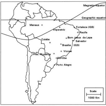
Fig. 1. RBMC stations - Brazil.
results of two campaigns, called GPS BRASION’91 (Brasil-Ionosphere) and BRASION’92. The regions of highest iono-spheric delay are located, on average, approximately±15◦ to±20◦ on either side of the earth’s geomagnetic equator (Klobuchar, 1991).
With the establishment of the Brazilian Network for Con-tinuous Monitoring of GPS satellites (RBMC) by the Funda¸c˜ao Instituto Brasileiro de Geografia e Estat´ıstica (IBGE), a very large data base becomes available to accom-plish studies related to the ionosphere in Brazilian conditions. Nowadays, RBMC is composed of 12 stations, collecting GPS data continuously. Two of these stations, in Bras´ılia and in Fortaleza, make part of IGS (International GPS Service) network. One of the main objectives of RBMC is its use as a reference for relative positioning. The network operates with dual frequency GPS receivers, except in the Fortaleza station, where a Rogue SNR-8000 receiver operates, the other sta-tions are equipped with Trimble 4000 SSI. They are located in Bom Jesus da Lapa/BA (BOMJ), Bras´ılia/DF (BRAZ), Cuiab´a/MT (CUIB), Curitiba/PR (PARA), Fortaleza/CE (FORT), Imperatriz/MA (IMPZ), Manaus/AM (MANA), Presidente Prudente/SP (UEPP) and Vi¸cosa/MG (VICO), Porto Alegre/RS (PORT), Recife/PE (RECF) and Salvador/BA (SALV) (Fig. 1).
The aim of this work is to define and establish a mathe-matical model that represents the Brazilian ionospheric con-ditions in order to provide capability to the single frequency GPS users to correct theirs observables from such effects. Data from RBMC provide the input to the model.
2.
Ionosphere
Considering the propagation aspects of the GPS signals, it is convenient to subdivide the atmosphere in troposphere and ionosphere, because the conditions of signal propaga-tion are different for each one. The layers closer to the earth atmosphere are called troposphere, which extends from the earth’s surface to about 50 km above the earth. It constitutes
molecules called ions. In this region the signal propagation depends on the frequency.
The GPS signals, on their path between satellites and re-ceivers, propagate through the dynamic atmosphere, and thus experience different kinds of influences. Variations may oc-cur in the direction of propagation, in the velocity of propaga-tion and in the signal strength. The ionosphere is a dispersive medium, meaning that the modulation on the carrier and the carrier phase are affected differently and that this effect is a function of carrier frequency. Therefore, these effects cause an increase and a decrease in the distances obtained from the code and carrier phase, but of the equal magnitude. Since the ionospheric effect depends on the frequency, consequently it depends on the refraction index as well. It is proportional to the total electron content (TEC), the number of electrons present along the path of the signal between the satellite and the receiver. The main problem is that TEC varies in time and space.
The refraction index of the phase (+) and group (−), con-sidering only the first order effects, is given by:
nf =1± 40.3ne
f2 , (1)
where neis the electron density, which is given in units of electrons per cubic meter and f is the frequency of the signal. For group delay of GPS signal arriving at station (r ) from satellite (s), the ionospheric refraction(Is
r)is given by (Leick, 1995):
Irs= 40.3
f2 TEC. (2)
3.
Ionospheric Correction for Positioning with
Single Receivers
Some methods have been used to determine the systematic effect due to ionospheric refraction in the L1 carrier of single frequency GPS receivers. The quantification of this effect can be evaluated by:
• Coefficients transmitted in the navigation messages— Klobuchar model;
• Observables collected with single frequency GPS re-ceivers;
• Observables collected with dual frequency GPS re-ceivers.
In this work the method that uses data from dual frequency, especially the pseudorange filtered by the carrier phase will be focused. In the derivation of the model, errors due to non-synchronism of the satellite and receiver clocks, ephemerides and the tropospheric refraction will be neglected, since their effects contaminate both frequencies in the same way and do not affect the validity of the results. The model is based on the difference between pseudoranges(Ps
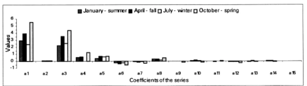
Fig. 2. Estimated average coefficients of the model.
and L1. It is given by (Georgiadiou, 1994):
P2rs−P1rs =I2rs −I1rs +(Sp2s −Ssp1)+(Rp2−Rp1)+ǫp21. (3)
Using Eq. (2) gives:
I2rs −I1rs =40.3TECs f 2 1 − f22
f12f22
=I1rs f
2 1 − f
2 2
f2 2
=I1rs 1
F, (4)
thus:
F(P2rs −P1rs)= I1rs +F [(Ssp2−Ssp1)+(Rp2−Rp1)] +Fǫp21. (5)
This equation is used to estimate the ionospheric slant delay(I1rs)in the L1 carrier, based on pseudorange observ-ables. The differences(Ssp2−Ssp1)and(Rp2−Rp1)represent, respectively, L1-L2 satellite and receivers interfrequency bi-ases, andǫp21represents another differential errors.
The model developed by Georgiadiou (1994) for model-ing the ionosphere was a contribution towards the develop-ment of a regional model based on GPS for the area cov-ered by the Active GPS Reference System (AGRS) of the Netherlands. It consists of a modification of the model de-veloped by Georgiadiou and Kleusberg (1988), to calculate the ionospheric L1 delay:
I1rs = I
v
1
cos(z′s), (6)
where Iv
1 represents the vertical ionospheric delay and z′s the zenital angle of the signal path from the satellite (s) to a point (ionospheric point) in an ionospheric layer of 400 km of height. Thus:
F(P2rs −P1rs)= I
v
1
cos(z′s)+F [(S s p2−S
s
p1)+(Rp2−Rp1)] +Fǫp21. (7)
The term on the left side of this equation represents the ionospheric delay in the L1 carrier, obtained from the mea-surements of the pseudoranges in both frequencies. Georgiadiou (1994) used the following series to represent the diurnal behavior of vertical ionospheric delay:
I1v =a1+a2Bs+ n
i=1 j=2i+1
{ajcos(i hs)+aj+1sin(i hs)}
+an∗2+3Bshs, (8)
Fig. 3. L1-L2 interfrequency bias average due to the receivers.
where the value of n depends on the significance of the pa-rameter.
The variable Bsis the difference between the receiver lat-itude and the latlat-itude of the subionospheric point (projection of a point on ionospheric layer upon the earth surface). The variable hsis given as:
hs= 2π
T (t−14
h), (9)
where T represents the period of 24 hours and t is the local time in hours, of the subionospheric point.
In the Georgiadiou (1994) experiments, only one receiver was used and the groups L1-L2 of the interfrequency biases (Cs = F [(Ss
p2−S s
p1)+(Rp2−Rp1)])were estimated for each satellite. In our experiment, where several receivers of RBMC were involved, the interfrequency biases of the satellite and the receivers were estimated separately. The total number of unknown parameters are 15+r+s, where
15 represent the coefficients of the series, r corresponds to the L1-L2 receivers interfrequency biases, which is equal to the number of network stations and s corresponds to the L1-L2 satellite interfrequency biases, being equal to the num-ber of tracked satellites. The numnum-ber of equations avail-able is greater than the number of unknown parameters, en-abling to apply the least-squares method. The design matrix A presents rank deficiency, equal to one (Camargo, 1999). Therefore, the L1-L2 receivers or satellites interfrequency biases have to be determined in relation to one of them.
4.
Experiments
anal-Fig. 4. L1-L2 interfrequency bias average due to the satellites.
ysis (Teunissen, 1985), as well as a test for the significance of the parameters used in the model (Zhong, 1997). The software allows estimating the coefficients of the model and can provide corrections to the L1 carrier observables. The observation files used to calculate the coefficients, as well as the ones corrected must be in the RINEX format. Therefore, the data processing can be carried out by any ordinary GPS software that accepts such a format.
In the experiments, data from 9 RBMC stations were used, with 30 seconds data rate. The ionosphere layer adopted was 400 km, and the observables used were the pseudorange fil-tered by the carrier phase, using the algorithm presented by Jin (1996). The filtering was used with the aim of handling the multipath error and the noise presented in the pseudor-anges observations. Only data collected above 15 degrees of elevation were used.
Tests with point positioning and relative positioning were accomplished. For the former, the data were processed with the software GPSPACE Version 3.2, developed by the Geode-tic Survey Division, Natural Resources Canada (NRCan, 1997). The baselines data used in the analysis were pro-cessed using the software GPSurvey Version 2.2 of Trimble.
4.1 Model parameter analysis
An analysis of the parameters of the model will be pre-sented in this section. The data used refer to four months of 1998, enclosing one-month of each four seasons.
In order to remove the L1 systematic effects of the ref-erence station, the average of the interfrequency biases of the satellites was calculated (F(Ss
p2−S s
p1)) and it was subtracted from the individual daily value of each satellite, because the average variation reflects the variation of the reference station (Sardon and Zarraoa, 1997). The interfre-quency biases of each satellite relative to the average are given by:
F(Ssp2−Ssp1)m=F(Ssp2−Ssp1)− F(Sp2s −Ssp1). (10)
Therefore, the interfrequency bias due to the receivers, relative to the average, is calculated as:
F(Rp2−Rp1)rm=F(Rp2−Rp1)r− F(Ssp2−S s
p1). (11)
This procedure, according to Sardon and Zarraoa (1997), removes the effect of the interfrequency bias of the reference station, but it does not make possible to obtain the absolute interfrequency biases of the satellites or the receivers in L1. Such values, related to the satellites, are transmitted in the broadcast messages. From April 1999, they are providing by JPL (Jet Propulsion Laboratory), since the values supplied
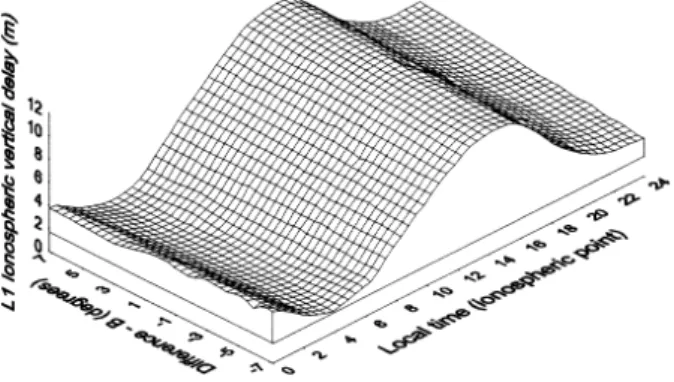
Fig. 5. Estimated Ionospheric vertical delays - UEPP station (274/1998).
by the satellite maker presented some problems (Wilson et
al., 1999).
Figures 2, 3 and 4 show, respectively, the coefficient aver-ages estimated from the model, the systematic L1 error due to the receivers and due to the satellites. These values represent the average estimated for each month.
The coefficients shown in Fig. 2, mainly a1and a3, provide an idea of the ionosphere seasonal behavior. There is a high ionosphere activity in the months of April (fall) and Octo-ber (spring), soon after the equinoxes, while it is smaller in January (summer) and July (winter), after the solstices. The precisions (1σ) of the daily coefficients averages were better than 0.019 m and for the monthly coefficients averages were better than 0.753 m. In the accomplished experiments, the order of the series given by Eq. (8), with n=6, was appro-priated. The significance test of the parameters showed that in 61% of the experiments the coefficients a13 and a14were not significant.
The maximum value of the receivers interfrequency biases occurred in January and October and the minimum in April and July (Fig. 3). The precisions of the daily and monthly averages were better than 0.027 m and 0.848 m. Concerning the systematic error of the satellites (Fig. 4), the individual average of each satellite showed a random behavior. The largest discrepancies mainly occurred in October. The daily and monthly precisions averages for L1-L2 satellites inter-frequency biases were, respectively, better than 0.061 m and 0.662 m.
4.2 Ionospheric vertical delay
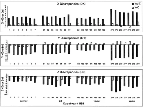
Fig. 6. Discrepancies between the “true” and the estimated cartesian coordinates of UEPP station (WoIC and WIC refer to the solution without and with ionospheric corrections).
ionospheric vertical delay resulting from the adopted model, as a function of the local time of the ionospheric point and of the difference (B) between the station latitude and the latitude of the sub-ionospheric point.
From Fig. 5 it can be observed that the daily maximum ionosphere activity occurs close to the 14:00 local time, as expected. The ionospheric quality model can be verified with a residual analysis, applying the GOM (Global Overall Model) (Teunissen, 1985). They presented average close to zero and standard deviation of 1.5 m, except in October, when the standard deviation was about 2.2 m. Based on the GOM statistic, the model was accepted with significance levelα equal to 5%.
4.3 Point positioning test
The quality of the implemented model can be analysed by comparing the results obtained with the adopted model, against a considered “ground truth”. As “ground truth”, the SIRGAS (Geocentric System of Reference to South America) coordinates of the UEPP station were considered. It is worth to mention that the UEPP station did not partic-ipate in the group of stations that provided data to estimate the parameters of the model. Therefore, it provides an inde-pendent result.
For point positioning from pseudorange observables (C/A), the data of the UEPP station during 1998 were used, enclosing one week of each seasons. The values estimated for the cartesian coordinates (X,Y,Z ) were daily compared
with corresponding the “ground truth”. It was considered the cases without ionospheric correction (WoIC) and with ionospheric correction (WIC).
The precise ephemerides and clock corrections of the satel-lites produced by GSD/NRCan were used. The objective was to eliminate the effects of SA that is the largest error source in the point positioning. In order to avoid estimated positions
with poor geometry, only GDOP (geometric dilution preci-sion) equal or smaller than 7 was used. In the processing, only pseudorange collected above 15 elevation degrees was considered, and the precision adopted was of 3.0 m. The meteorological data used for tropospheric corrections were collected in the FCT/Unesp meteorological station, close to the UEPP station.
Figure 6 shows the discrepancies among the considered “true” cartesian coordinates of the UEPP station and the es-timated ones (WoIC and WIC) for a 24-hour period.
The mean discrepancies for the processing WIC indicated discrepancies with respect to the ground truth better than a meter. Considering the resulting error ((D X2+DY2+D Z2), there was an error reduction of about 80%. It represents a mean error reduction from 8.44 m to 1.61 m. While the maximum error WoIC was 14.21 m, it was reduced to 5.33 m in the WIC processing. Considering the minimum error, the reduction was from 2.96 m (WoIC) to 0.55 m (WIC).
The discrepancies in the results obtained in an epoch per epoch solution for the first day of October are shown in Fig. 7. In the epoch per epoch solution, the results present the diurnal behavior of ionospheric delay (WoIC) and the im-proved results (WIC) for a 24-hour period. The maximum ionosphere effects occur, as expected, at 17 hours GPS time (∼=14 hours local time).
4.4 Relative positioning test
Further experiments were carried out in order to analyze the implemented model, considering now relative position-ing. Baselines of approximately 100 km were processed in relation to the UEPP station. All RBMC stations participated in the estimation of the parameters of the model.
Fig. 7. An epoch per epoch solution (274/1998)—discrepancies between the “true” and the estimated cartesian coordinates of UEPP station (WoIC and WIC refer to the solution without and with ionospheric corrections).
Fig. 8. Discrepancies between the “true” and the estimated distances (WoIC and WIC refer to the solution without and with ionospheric corrections).
For such cases, the double difference ionospheric free linear combination (ion free) was used as basic observable. The processing was carried out using the GPSurvey Software.
Again, two kinds of processing were carried out: WoIC and WIC. In both cases, IGS precise ephemerides and the Hopfield tropospheric model were used. Only observables with elevation angle larger than 15 degrees were used.
Figure 8 shows the discrepancies in distances between the baselines processed with ion free and L1 WoIC and L1 WIC. From Fig. 8 one may conclude that there was an error reduction of the order of 50% after corrections were applied.
5.
Conclusion and Future Work
A model for computing the effects of the ionosphere was presented. The experiments showed that this model provides an error reduction of 80%, in relation to the point positioning carried out without correction. Metric accuracy was achieved for most cases. Considering an epoch per epoch solution, the results showed that the model improves the results even during the daily ionosphere maximum (17 hours GPS time ≈14 hours local time).
For relative positioning the improvement was 50% for baselines of approximately 100 km. Further studies related to improvement of L1 relative positioning should be performed, trying to identify the main drawbacks in such cases.
Additionally, new functions to model the ionospheric de-lay should be tested, such as spherical harmonic and polyno-mial. Besides this, tests will be accomplished considering the variation of the ionospheric shell height, taking into account both the temporal and spatial variability of the ionosphere in the equatorial region. Also, tests with data that will be collected during the period of maximum solar activity, iono-spheric scintillation and magnetosphere substorm event will be accomplished. It is also our aim to produce ionospheric maps representing the ionospheric L1 carrier delay or TEC, for South America Region.
Considering the variability of the ionosphere in the equato-rial region, it is recommended to study other zenith mapping functions to project the line-of-sight ionosphere delay into the vertical and to analyze the impact of ionospheric map-ping function used in the proposed approach.
Acknowledgments. This work was developed with financial sup-port of FAPESP (contract 95/08775-1) and CAPES/PICD.
References
Camargo, P. O., Modelo Regional da Ionosfera para uso em Posicionamento com Receptores de uma Freq¨uˆencia, Ph.D. Thesis, Universidade Federal do Paran´a, 191 pp., 1999.
Campos, M. A., L. Wanninger, and G. Seeber, Condi¸c˜oes ionosf´ericas per-turbadas e os sinais GPS, 3o. Congresso Internacional da Sociedade Brasileira de Geof´ısica, Rio de Janeiro, pp. 601–604, 1993.
Georgiadiou, Y., Modeling the ionosphere for an active control network of GPS stations, in LGR-Series - Publications of the Delft Geodetic
Com-puting Centre, Delft University of Technology, n. 7, 1994.
1998.
Jin, X. X., Theory of carrier adjusted DGPS positioning approach and some experimental results, Ph.D. Thesis, Delft University of Technol-ogy, 162 pp., 1996.
Klobuchar, J. A., Ionospheric time-delay algorithm for single-frequency GPS users, IEEE Transactions on Aerospace and Electronic Systems, AES-23(3), 325–331, 1987.
Klobuchar, J. A., Ionospheric effects on GPS, GPS World, April, 48–50, 1991.
Leick, A., GPS Satellite Surveying, 560 pp., John Wiley & Sons, New York, 1995.
Monico, J. F. G., High Precision GPS Inter-continental Networks, Ph.D. Thesis, University of Nottingham, 205 pp., 1995.
Newby, S. P. and R. B. Langley, Three alternative empirical ionospheric models—are they better than GPS broadcast model?, in Proceedings
of the Sixth International Geodetic Symposium on Satellite Positioning,
pp. 240–244, Columbus, 1992.
NRCan, User’s Guide—GPSPACE (GPS Positioning from ACS Clocks and
Ephemerides—Version 3.2), Canadian Active Control System
Opera-tions, Geodetic Survey Division, Geomatics Canada, Natural Resources Canada, 1997.
Sardon, E. and N. Zarraoa, Estimation of total electron content using GPS data: how stable are the differential satellite and receiver instrumental
biases, Radio Sci., 32, 1899–1910, 1997.
Teunissen, P. J., Quality control in geodetic networks, in Optimization and
Design of Geodetic Networks, pp. 526–547, Berlin, 1985.
Wanninger, L., G. Seeber, and M. A. Campos, Use of GPS in the south of Brazil under severe ionospheric conditions, in IAG Symposium III, 10 pp., Heidelberg, 1991.
Wanninger, L., G. Seeber, and M. A. Campos, Limitations of GPS in equa-torial regions due to the ionosphere, VII Simp´osio Brasileiro de Sensori-amento Remoto, 14 pp., Curitiba, 1993.
Wells, D., N. Beck, D. Delikaraoglou, A. Kleusberg, E. J. Krakiwsky, G. Lachapelle, R. B. Langley, M. Nakiboglu, K. P. Schwarz, J. M. Tranquilla, and P. Vanicek, Guide to GPS Positioning, Canadian GPS Associates, Fredericton, New Brunswick, Canada, 1986.
Wilson, B. D., C. H. Yinger, W. A. Feess, and C. Shank, New and improved the broadcast interfrequency biases, GPS World, September, 56–66, 1999. Zhong, D., Robust estimation and optimal selection of polynomial parameter for the interpolation of GPS heights, Journal of Geodesy, 9(71), 552–561, 1997.