Analysis of groundwater drought using a variant of the Standardised Precipitation Index

(1)

HESSD

10, 7537–7574, 2013

Analysis of groundwater drought using a variant of SPI

J. P. Bloomfield and B. P. Marchant

Title Page

Abstract Introduction

Conclusions References

Tables Figures

◭ ◮

Back Close

Full Screen / Esc

Printer-friendly Version Interactive Discussion

Discussion

P

a

per

|

Di

scussion

P

a

per

|

Discussion

P

a

per

|

Discussi

on

P

a

per

|

Hydrol. Earth Syst. Sci. Discuss., 10, 7537–7574, 2013 www.hydrol-earth-syst-sci-discuss.net/10/7537/2013/ doi:10.5194/hessd-10-7537-2013

Geoscientiic Geoscientiic

Hydrology and Earth System

Sciences

Open Access

Discussions

This discussion paper is/has been under review for the journal Hydrology and Earth System Sciences (HESS). Please refer to the corresponding final paper in HESS if available.

Analysis of groundwater drought using a

variant of the Standardised Precipitation

Index

J. P. Bloomfield1and B. P. Marchant2

1

British Geological Survey, Maclean Building, Crowmarsh Gifford, Wallingford, Oxfordshire, OX10 8BB, UK

2

British Geological Survey, Environmental Science Centre, Keyworth, Nottingham, NG12 5GG, UK

Received: 21 May 2013 – Accepted: 3 June 2013 – Published: 14 June 2013 Correspondence to: J. P. Bloomfield (jpb@bgs.ac.uk)

(2)

HESSD

10, 7537–7574, 2013

Title Page

Tables Figures

◭ ◮

Back Close

Full Screen / Esc

Discussion

P

a

per

|

Di

scussion

P

a

per

|

Discussion

P

a

per

|

Discussi

on

P

a

per

|

Abstract

A new index for standardising groundwater level time series and characterising ground-water droughts, the Standardised Groundground-water level Index (SGI), is described. The SGI

is a modification of the Standardised Precipitation Index (SPI) that accounts for di_ff

er-ences in the form and characteristics of precipitation and groundwater level time series. 5

The SGI is estimated using a non-parametric normal scores transform of groundwater level data for each calendar month. These monthly estimates are then merged to form a continuous index. The SGI has been calculated for 14 relatively long, up to 103 yr, groundwater level hydrographs from a variety of aquifers and compared with SPI for the same sites. The SPI accumulation period which leads to the strongest correlation 10

between SPI and SGI,qmax, varies between sites. There is a positive linear correlation

betweenqmaxand a measure of the range of significant autocorrelation in the SGI

se-ries,mmax. For each site the strongest correlation between SPI and SGI is in the range

0.7 to 0.87, and periods of low values of SGI coincide with previously independently documented droughts. Hence SGI is taken to be a robust and meaningful index of 15

groundwater drought. The maximum length of groundwater droughts defined by SGI is

an increasing function ofmmax, meaning that relatively long groundwater droughts are

generally more prevalent at sites where SGI has a relatively long autocorrelation range.

Based on correlations betweenmmax, average unsaturated zone thickness and aquifer

hydraulic diffusivity, the source of autocorrelation in SGI is inferred to be dependent on

20

aquifer flow and storage characteristics. For fractured aquifers, such as the Cretaceous Chalk, autocorrelation in SGI is inferred to be primarily related to autocorrelation in the recharge time series, while in granular aquifers, such as the Permo-Triassic Sand-stones, autocorrelation in SGI is inferred to be primarily a function of intrinsic aquifer characteristics. These results highlight the need to take into account the hydrogeologi-25

(3)

HESSD

10, 7537–7574, 2013

Title Page

Tables Figures

◭ ◮

Back Close

Full Screen / Esc

Discussion

P

a

per

|

Di

scussion

P

a

per

|

Discussion

P

a

per

|

Discussi

on

P

a

per

|

1 Introduction

Drought is a costly natural hazard affecting socio-economic activity and agricultural

livelihoods as well as adversely impacting public health, and threatening the

sustain-ability of many natural environments (Wilhite, 2000; Fink et al., 2004; She_ffield and

Wood, 2008; Calow et al., 2010; Mishra and Singh, 2010). Droughts typically develop 5

slowly and can last from months to a few years (Santos, 1983; Lloyd-Hughes and Saun-ders, 2002; Tallaksen and van Lanen, 2004; Tallaksen et al., 2009). As highlighted in a recent review of drought concepts by Mishra and Singh (2010), groundwater droughts are of particular interest due to the manner in which drought propagates through hy-drological systems. During the early stages of a drought, as deficits are developing in 10

surface water and unsaturated zone stores, groundwater sources can provide relatively resilient water supplies and will sustain surface flows through groundwater baseflow (Hughes et al., 2012). Conversely, groundwater may be highly susceptible to relatively persistent or prolonged droughts, because, compared with surface water resources, groundwater storage may take significantly longer to be replenished and recover as 15

a drought begins to break.

A number of studies have sought to develop a better understanding of groundwater droughts in the context of meteorological drivers and, in particular, how droughts prop-agate through hydrological systems (Eltahir and Yeh, 1999; Peters et al., 2003, 2005, 2006; Tallaksen et al., 2006, 2009; van Lanen and Tallaksen, 2007; Leblanc et al., 20

2009). These studies have usually focussed on the catchment scale and have brought process understanding to bear on the evolution of groundwater droughts. Fewer studies have concentrated on regional characterisation of groundwater droughts, emphasis-ing monitoremphasis-ing, characterisation of longer-term trends and the development of drought warning systems (Chang and Teoh, 1995; Bhuiyan et al., 2006; Mendicino et al., 2008; 25

Fiorillo and Guadagno, 2010, 2012). A common feature of these latter studies is the need to develop relatively simple but consistent measures or indices of the status of

(4)

HESSD

10, 7537–7574, 2013

Title Page

Tables Figures

◭ ◮

Back Close

Full Screen / Esc

Discussion

P

a

per

|

Di

scussion

P

a

per

|

Discussion

P

a

per

|

Discussi

on

P

a

per

|

aquifers and catchments at the regional scale, as well as that enable groundwater drought to be compared with other hydro-meteorological aspects of drought. Despite the previous work, there are still no commonly accepted indices to quantify

groundwa-ter droughts, so making it difficult to incorporate groundwater drought phenomena into

wider drought assessments. To address this shortcoming, here we present for the first 5

time a systematic assessment of how one of the most commonly used hydrological drought indices, the Standardised Precipitation Index (SPI), can be applied to ground-water level data in order to define a new groundground-water level index for use in groundground-water drought monitoring and analysis.

Context for development of the SGI

10

Many drought indices have been developed in recent decades to enable drought sever-ity, duration and spatial extent to be characterised and compared in a standardised manner (Panu and Sharma, 2000; Mishra and Singh, 2010). Mishra and Singh (2010) provide a commentary on the strengths and weaknesses of a number of these indices as well as on their comparative performance. One of the most widely used indices is 15

the SPI, (McKee et al., 1993; Edwards and McKee, 1997). The SPI was originally de-veloped as a simple method for characterising meteorological drought. It consists of a normalised index obtained by fitting a parametric distribution function to long-term precipitation records and is calculated for a range of rainfall accumulation periods or time scales. As noted by McKee et al. (1993), it is potentially applicable to any hydro-20

metric series, including groundwater levels, which reflects changes in the state of water resources. Consequently, variants of the SPI methodology have been applied to other aspects of the hydrological system such as surface flows, reservoir storage and soil moisture (e.g. Vincente-Serrano and Lopez-Moreno, 2005; Shukla and Wood, 2008; Nalbantis and Tsakiris, 2009;) as well as studies of groundwater droughts (Bhuiyan 25

(5)

HESSD

10, 7537–7574, 2013

Title Page

Tables Figures

◭ ◮

Back Close

Full Screen / Esc

Discussion

P

a

per

|

Di

scussion

P

a

per

|

Discussion

P

a

per

|

Discussi

on

P

a

per

|

Deployable output from water supply boreholes is a function of groundwater level. Hence, if an appropriate standardised index can be applied, groundwater levels at ob-servation boreholes are a useful measure of the quantitative status of groundwater

resources during a regional drought. As will be shown, differences in the form and

characteristics of the different types of hydrometric time series require modifications

5

to be made to the SPI methodology of McKee (McKee et al., 1993; Edwards and Mc-Kee, 1997) if the methodology is to be applied to groundwater level hydrographs and so to the analysis of groundwater droughts. In this paper issues related to the applica-tion of the SPI to groundwater level time series are addressed, and a modificaapplica-tion to the SPI methodology is presented that enables monthly groundwater level time series 10

to be used as the basis for estimating a new Standardised Groundwater level Index (SGI). The SGI is calculated for groundwater level hydrographs from 14 sites across the United Kingdom (UK), where sites have been selected from a range of aquifer types and to exhibit a range of hydrograph characteristics. The relationships between SPI and SGI at the study sites are investigated and quantified using correlation anal-15

ysis. Groundwater droughts at the study sites are then identified and described using the SGI time series and the influence of some possible hydrogeological explanatory factors on SGI is explored.

2 Study sites and data

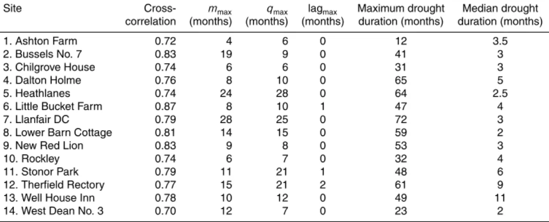
Groundwater level hydrographs from 14 sites across the UK have been used in the 20

study. The sites are part of the UKs long-term observation borehole network, consist of a broad range of unconfined consolidated aquifers types and are not significantly

a_ffected by pumping (Bloomfield et al., 2009). The sites include those located on the

Lincolnshire Limestone, a fractured limestone aquifer (Allen et al., 1997); the Chalk aquifer, a dual porosity, dual permeability carbonate aquifer with local karstic devel-25

(6)

inter-HESSD

10, 7537–7574, 2013

Title Page

Tables Figures

◭ ◮

Back Close

Full Screen / Esc

Discussion

P

a

per

|

Di

scussion

P

a

per

|

Discussion

P

a

per

|

Discussi

on

P

a

per

|

grannular flow predominates. Figure 1 shows the location of the observation boreholes in relation to the major aquifers in the UK, and summary information about the sites and groundwater hydrographs is given in Table 1, where all groundwater levels in Table 1 and subsequent figures is reported as metres above mean sea level.

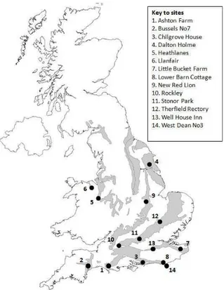
Monthly groundwater level data for the study sites has been taken from the UK Na-5

tional Groundwater Level Archive (National Groundwater Level Archive, 2013). The monthly groundwater level records range in length from 29 to 103 yr. Figure 2 is a plot of the monthly groundwater level hydrographs for the 14 sites, where all hydrographs are drawn to the same scale. Precipitation data has been derived from two sources. For 1961 to the end of 2005 precipitation data is taken from the Centre for Ecology and 10

Hydrology’s CERF 1 km gridded precipitation dataset (Keller et al., 2005). Pre-1961

monthly precipitation data has been taken from the Meteorological Office Integrated

Data Archive System, MIDAS (BADC, 2013). The rainfall records are combined to give a continuous precipitation record at each site. An example of a precipitation time se-ries is given in Fig. 3. It shows one month accumulated precipitation for Dalton Holme 15

plotted with the corresponding monthly groundwater level. Average annual precipitation varies between sites from 580 to 1100 mm (Table 1).

3 Statistical methods

3.1 Development of a new Standardized Groundwater Index (SGI)

The SPI was proposed by McKee et al. (1993) as an objective precipitation-based 20

measure of the severity and duration of droughts. McKee et al. (1993) suggested that drought status could be described by a normally distributed index. The index was fit-ted to a time series of the recorded precipitation at a site for accumulation periods of 3, 6, 12, 24 and 48 months. The calculation of the SPI requires three steps. First a gamma distribution is fitted to the time series of accumulated precipitation observed 25

(7)

HESSD

10, 7537–7574, 2013

Title Page

Tables Figures

◭ ◮

Back Close

Full Screen / Esc

Discussion

P

a

per

|

Di

scussion

P

a

per

|

Discussion

P

a

per

|

Discussi

on

P

a

per

|

i is the number of months since the start of the time series andnis the total number

of observations. For eachi =1, 2,. . .,n, McKee et al. (1993) then used the fitted

dis-tribution to determinep_i, the probability that a value drawn at random from the fitted

distribution was less than or equal tozi. Finally McKee et al. (1993) applied the inverse

normal cumulative distribution function (with mean zero and variance one) to thesepi

5

to yield a lengthn time series of SPI values denoted here as SPI_q(i), whereq is the

number of months over which rainfall is accumulated. The resulting SPI is a contin-uous variable, however, McKee et al. (1993) also arbitrarily defined drought intensity

according to the SPI where they denoted SPI≤ −2 corresponding to extreme drought,

−1.5≥SPI>−2 corresponding to severe drought, −1.0≥SPI>−1.5 corresponding

10

to moderate drought, 0_≥SPI>−1 corresponding to minor drought and SPI>0

corre-sponding to no drought.

It would be possible to calculate a Standardized Groundwater Index (SGI) by exactly the same method using monthly groundwater levels instead of accumulated

precipita-tion. However, some differences between observed groundwater level hydrographs and

15

precipitation time series should be borne in mind. Firstly, groundwater level is a con-tinuous variable and there is no need to accumulate it over a specified time period. Secondly, a much stronger seasonal pattern of variation is evident in UK groundwater levels than is seen in accumulated precipitation values (Fig. 3). If the SPI methodology were naively followed using such strongly seasonal data then the resultant SGI may 20

appear to include regular droughts each summer and therefore this seasonal trend must be removed from the data prior to calculation of a meaningful SGI. This could be achieved by fitting a periodic model of the annual variation in groundwater levels. The SGI, however, may still be unduly influenced by deviations of the data from a simple

periodic model and a more effective way to remove the seasonal effect is to estimate

25

(8)

HESSD

10, 7537–7574, 2013

Title Page

Tables Figures

◭ ◮

Back Close

Full Screen / Esc

Discussion

P

a

per

|

Di

scussion

P

a

per

|

Discussion

P

a

per

|

Discussi

on

P

a

per

|

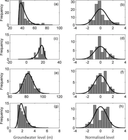
months at four of the study sites – (a) Chilgrove House in November, (c) New Red Lion in April, (e) Therfield Rectory in May and (g) West Dean No. 3 in June. The four

histograms differ in the sign and magnitude of their skewness. Therefore distribution

functions which can represent more general behaviour than the gamma distribution are required to model variations in the form of monthly distributions of groundwater 5

levels.

We initially fitted normal, log-normal, gamma and extreme-value distributions to the monthly groundwater levels at each site by maximum likelihood (MATLAB, 2012). These distributions were selected because they can accommodate all magnitudes of non-negative skewness from zero to severe. Negative skewness was accommodated 10

by applying a shift z∗_i =c−zi for constant c to the data prior to fitting the

distribu-tion. Figure 4 (left panels) shows the best-fitting distribution functions according to the Akaike information criterion (Akaike, 1973) for the four example histograms and the corresponding plots on the right show the SGI which results. The best-fitting

distri-bution function is different in each case. For Chilgrove House in November it is the

15

gamma distribution. For New Red Lion in April it is the negatively skewed extreme value distribution and for Therfield Rectory in May and West Dean No. 3 in June it is the log-normal and extreme value distributions respectively. Figure 4 (right panels) shows that the quality of the computed SGIs also appears to vary in regards to how well the estimated values of SGI correspond to the normal distribution of zero mean 20

and standard deviation of one. The quality of the estimated values of SGI for all months at all 14 sites have been estimated by applying the Kolmogorv–Smirnov test for nor-mality (Everitt, 2002). The results are highly variable, with one distribution of SGI, for

Chilgrove House in November, failing the K–S test at thep=0.05 level. Given the

vari-ation in the degree to which these SGI estimated from parametric models conform to 25

the normal distribution it is doubtful whether they can be objectively compared.

(9)

HESSD

10, 7537–7574, 2013

Title Page

Tables Figures

◭ ◮

Back Close

Full Screen / Esc

Discussion

P

a

per

|

Di

scussion

P

a

per

|

Discussion

P

a

per

|

Discussi

on

P

a

per

|

their rank within a dataset, in this case groundwater levels for a given month from a given hydrograph. We note that a related non-parametric method, the plotting posi-tion method, has previously been used by Osit et al. (2008) to estimate standardised precipitation for comparison with SPI. The normal scores transform is undertaken by

applying the inverse normal cumulative distribution function tonequally spacedpi

val-5

ues ranging from 1/2nto 1−1/2n. The values that result are the SGI values. They

are then re-ordered such that the largest SGI value is assigned to thei for whichp_i is

largest, the second largest SGI value is assigned to thei for whichpi is second largest

and so on. The SGI distribution which results from this transform will always pass the K–S normality test.

10

In some statistical applications it is undesirable to use a normal scores transform because the model is over-fitted. This means that the model matches the particular intricacies of the existing observed data to a degree that will not be achieved on in-dependently gathered observations of the same property. This could mean that the uncertainty of a prediction of the property at a time when it was not measured is 15

under-estimated. However, we wish to use the normal scores data to describe existing observations rather than to predict values. Therefore we need not be concerned by over-fitting even if it is present for some of the normal scores transforms.

In summary, for each of the 14 study sites, normalized indices are estimated from the groundwater level data for each calendar month using the normal scores transform. 20

These normalized indices are then merged to form a continuous SGI. The SPI is es-timated directly for the entire time series rather than splitting the series into calendar

months. At each site SPI is estimated with accumulation periods of 1, 2,. . ., 24 months.

To ensure consistency between groundwater and precipitation indices SPIs are also estimated using the normal scores transform.

(10)

HESSD

10, 7537–7574, 2013

Title Page

Tables Figures

◭ ◮

Back Close

Full Screen / Esc

Discussion

P

a

per

|

Di

scussion

P

a

per

|

Discussion

P

a

per

|

Discussi

on

P

a

per

|

3.2 Methods used to analyse SGI, correlations with SPI and hydrogeological factors influencing the drought indices

In order to quantify groundwater droughts using the SGI, we are interested in charac-terising the autocorrelation in SGI time series. Autocorrelation can be quantified using a correlogram (Diggle, 1990). If we denote the mean SGI for the borehole by SGI then 5

thek-th sample autocovariance coefficient is defined to be

g_k=_n1 n X

i=k+1

n

SGI(i)−SGIo nSGI(i−k)−SGIo (1)

and thek-th sample autocorrelation coefficient is

rk=

g_k g0

. (2)

The correlogram is a plot ofr_k againstk. If there is no correlation between the SGI(i)

10

observed k months apart and if the SGI values are normally distributed then rk is

approximately normally distributed with mean zero and variance 1/n. Therefore values

ofr_kwith magnitude greater than 2/√nsuggest significant correlation at approximately

the 5 % level. We define the range of significant temporal correlation for a SGI to be the largestm,mmax, for whichrk>2/

√

nfor allk≤m. The threshold on the autocorrelation

15

coefficients which signifies significant correlation will vary according to the length of the

time series. Since we wish to use a common threshold for all of our SGI series to enable comparison between sites we have selected 0.11 as the SGI autocorrelation threshold,

tSGI, since this is the significant threshold (p=0.05) for our shortest SGI time series

(for Lower Barn Cottage with a record length of 29 yr). 20

In addition, linear correlation coefficients have also been calculated to quantify the

strength of relationships between SPI and SGI, and betweenmmax and possible

ex-planatory variables. These exex-planatory variables, including unsaturated zone

(11)

HESSD

10, 7537–7574, 2013

Title Page

Tables Figures

◭ ◮

Back Close

Full Screen / Esc

Discussion

P

a

per

|

Di

scussion

P

a

per

|

Discussion

P

a

per

|

Discussi

on

P

a

per

|

(T/S) have been estimated for each site and are listed in Table 1. Note that no

pump-ing test data is available for any of the study sites, soT and S values are estimates

based on mean values derived from pumping tests for a given region and aquifer com-bination as reported by Allen et al. (1997). An exception is that unconfined storage

coefficients for sites on the Permo-Trias sandstone aquifer are estimated to be 0.1

5

(also after Allen et al., 1997). This is because, as Allen et al. (1997) note, estimates

ofS from short-term pumping tests on this aquifer typically significantly underestimate

long-term storage and a value of 0.1 for S has been taken as the optimal value for

long-term storage.

4 Results

10

4.1 Estimated SGI and SPI

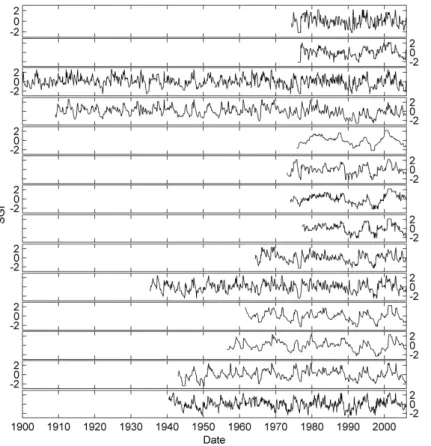
Estimated monthly SGI for each of the 14 study sites are given in Fig. 5. In the present

study SPI has been estimated forq=1, 2,. . ., 24 months. However, SPI is usually only

calculated and reported for selected periods. So for simplicity and to illustrate how SPI

varies withqat one of the study sites, Fig. 6 shows SPI for Dalton Holme forq=1, 3,

15

6, 12 and 24 months. Figure 6 also includes the SGI time series for Dalton Holme for comparison with the SPI time series.

Compared with the raw groundwater level data, Fig. 2, the SGI data does not con-tain a strong seasonal component, Fig. 5, and unlike the groundwater level time series, the SGI time series show many similar broad-scale structures across all the sites. For 20

example, all sites show generally low values of SGI in the early 1990s, with SGI increas-ing in the mid-1990s and then decreasincreas-ing again in the later 1990s. There are, however,

differences in the short-range variation in SGI between sites. For example, the SGI for

Ashton Farm, Chilgrove House and West Dean No. 3 appear to be considerably

nois-ier than Therfield Rectory, Stonor Park or Llanfair DC. This reflects differences in the

25

(12)

HESSD

10, 7537–7574, 2013

Title Page

Tables Figures

◭ ◮

Back Close

Full Screen / Esc

Discussion

P

a

per

|

Di

scussion

P

a

per

|

Discussion

P

a

per

|

Discussi

on

P

a

per

|

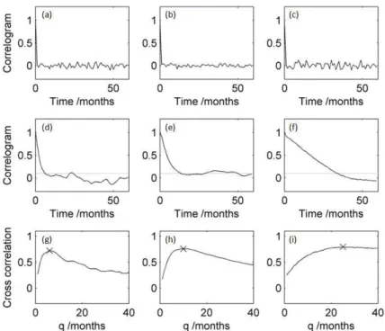
plots of SGI autocorrelation as a function of lag in months (solid lines) for three exam-ple sites, Ashton Farm, Dalton Holme and Llanfair DC, with contrasting autocorrelation.

Using the SGI autocorrelation threshold, tSGI, of 0.11 (the dashed line in the figure),

the SGI autocorrelation range (mmax) for each of the sites has been estimated and is

given in Table 2. Table 2 shows that significant temporal autocorrelation in SGI,mmax,

5

varies between sites, from as little as 4 months at Ashton Farm up to 28 months at Llanfair DC.

As has been noted by McKee et al. (1993) and in previous studies (Vincente-Serrano and Lopez-Moreno, 2005), the degree of noise or short-range variation in SPI varies as a function of the precipitation accumulation period. This is also seen in the present 10

study. For example, the SPI for Dalton Holme is relatively noisy whenq=1 compared

with SGI Fig. 6, and Fig. 7 (middle panels) shows the very short autocorrelation range

for SPI (q=1) at the three example sites. However, SPI becomes smoother and less

noisy and long-range correlations become more prominent as precipitation accumula-tion periods increase, Fig. 6.

15

4.2 Correlation between SPI and SGI

The cross-correlation between SPI and SGI for SPI accumulation periods of q=

1, 2,. . ., 24 has been computed and is shown for three representative sites in Fig. 7

(bottom panels). At each site a maximum correlation associated with an optimum SPI

accumulation period can be identified and is denoted by anX on each of the

cross-20

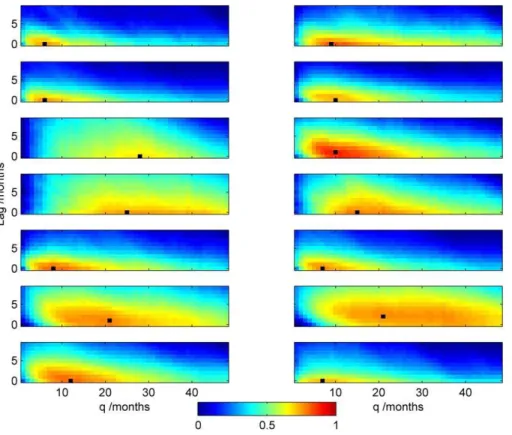
correlation curves. However, investigation of the cross-correlation co-e_fficients for

a range of lags between SPI and SGI shows that the maximum correlation may not nec-essarily occur at a lag of zero months. So for all sites the cross-correlation between SPI

and SGI has been estimated for SPI accumulation periods ofq=1, 2,. . ., 24 months

and for lags of one month increments up to 24 months. The resulting cross-correlations 25

(13)

as-HESSD

10, 7537–7574, 2013

Title Page

Tables Figures

◭ ◮

Back Close

Full Screen / Esc

Discussion

P

a

per

|

Di

scussion

P

a

per

|

Discussion

P

a

per

|

Discussi

on

P

a

per

|

sociated with lag zero, however, at Little Bucket Farm, Therfield Rectory and Stonor, the maximum correlation is associated with lags of 1, 1, and 2 months respectively. Table 2 lists the values of the maximum cross-correlation between SPI and SGI, as

well as associated the accumulation period (qmax) and associated lag. The maximum

cross-correlations between SPI and SGI are generally strong with coefficients typically

5

in the range 0.7 to 0.87, Table 2, with the highest coefficient of 0.87 associated with the

site at Little Bucket Farm and the lowest coefficients of 0.7 associated with the site at

West Dean No. 3 – both sites being on the Chalk aquifer. Plots of SGI as a function of

SPIqmax show that for all sites there is a linear relationship between the two drought

indices, Fig. 9. 10

The SPI accumulation period associated with the maximum cross-correlations,qmax,

and the SGI autocorrelation range,mmax, both vary between sites and broadly increase

in the same order for the study sites. Whenqmaxis plotted againstmmax, Fig. 10, there

is an approximate one-to-one relationship with correlation coe_fficient of 0.79 that is

significant forp <0.001. 15

4.3 Groundwater droughts as defined by SGI

Cole and Marsh (2006) and Marsh et al. (2007) identified seven episodes of major droughts in England and Wales during the period covered by the groundwater level records investigated in the present study. They noted that all the droughts had large geographical footprints extending over much of England and Wales and in some cases 20

a_ffecting the whole of the UK, but that regional variations in drought intensities are

present within and between the major drought events. Of these major droughts, they estimated that all but one had sustained and or severe impacts on groundwater levels. Marsh et al. (2007) also noted that a number of the droughts were characterised by transitions from initial surface water stress to lowered groundwater heads at the na-25

(14)

HESSD

10, 7537–7574, 2013

Title Page

Tables Figures

◭ ◮

Back Close

Full Screen / Esc

Discussion

P

a

per

|

Di

scussion

P

a

per

|

Discussion

P

a

per

|

Discussi

on

P

a

per

|

and includes a brief commentary after Marsh et al. (2007) on the individual drought characteristics.

Figure 11 is a re-presentation of the SGI data from Fig. 5 as a heat map, where

non-drought periods, SGI>0, are shown in grey, and drought periods, SGI<0, are

shown in shades of yellow through to red with decreasing SGI, i.e. with increasing 5

drought intensity. Figure 11 is consistent with the observations of Marsh et al. (2007) that the UK has experienced a number of major groundwater droughts. In particular, the droughts of 1976, 1990 to1992, and 1995 to 1997 are clearly expressed by the SGI records at the majority of sites. Groundwater droughts prior to the early 1970’s are less easy to discern as there are fewer records. In addition, the following specific 10

observations can be made:

– There is no evidence in the SGI data to support a significant groundwater

compo-nent to the 1959 drought episode, however, this is consistent with the observation of Marsh et al. (2007) that this drought had modest groundwater impact.

– The 1933–1934 drought episode appears prominently in the SGI records at

15

Chilgrove House, but is absent from the record at Dalton Holme suggesting that it may have been less significant in the northern part of the region.

– The 1921–1922 drought episodes appear in the SGI records at both Chilgrove

House, and Dalton Holme.

– There is some evidence from the Chilgrove House record for short drought

20

episodes between 1900 and 1910 as part of the 1890–1910 “Long Drought”.

– In addition, the SGI records indicate that groundwater drought conditions not

pre-viously identified by Marsh et al. (2007) were experienced at a number of sites during the mid-1960s, and the mid- and late 1940s.

Based on these observations, SGI appears to record groundwater drought response to 25

(15)

HESSD

10, 7537–7574, 2013

Title Page

Tables Figures

◭ ◮

Back Close

Full Screen / Esc

Discussion

P

a

per

|

Di

scussion

P

a

per

|

Discussion

P

a

per

|

Discussi

on

P

a

per

|

as adding apparent refinements to the drought history. Figure 11 is also consistent with the assertion of Marsh et al. (2007) that many of the hydrometric droughts in England and Wales have a wide geographic impact. Sites at the geographical extent of the study area, such as Dalton Holme in the northeast, Llanfair DC in the northwest, Bussels No. 7 in the southwest, and Little Bucket Farm in the southeast, all record 5

drought events in the form of anomalously low SGI values for the droughts of 1976, 1990 to 1992 and 1995 to 1997.

5 Discussion

The SGI autocorrelation varies significantly between sites, but given that one of the purposes of developing a groundwater drought index is to compare standardised mea-10

sures of drought between sites, what are the implications, if any, of this observation? For example, it may be expected that the autocorrelation structure of SGI will influence the length of groundwater droughts recorded at a given site, where sites with relatively long significant SGI autocorrelations might experience a limited number of relatively long droughts and sites with relatively short significant SGI autocorrelations may expe-15

rience more numerous but briefer episodes of groundwater drought. How doesm_max

influence temporal patterns of groundwater drought at a site, and if mmax influences

groundwater drought response, what are the possible causes of or controls onmmax?

5.1 The relationship betweenmmaxand drought duration

To investigate the effect of autocorrelation in SGI on groundwater drought, here we

as-20

sume that, as a first-order approximation, the broad meteorological drought history of the study sites is spatially homogeneous and investigate how drought duration defined

by SGI varies between sites as a function ofm_max. This assumption means that any

comparative differences in drought characteristics between sites would need to be

ex-plained in terms of intrinsic differences in the SGI time series, rather than differences in

(16)

HESSD

10, 7537–7574, 2013

Title Page

Tables Figures

◭ ◮

Back Close

Full Screen / Esc

Discussion

P

a

per

|

Di

scussion

P

a

per

|

Discussion

P

a

per

|

Discussi

on

P

a

per

|

the drought climatology. This assumption has been justified on the grounds that Marsh et al. (2007) noted that all the major hydrological drought episodes in England and

Wales affected “almost all of the UK”, i.e. covering an area significantly greater than

that defined by the sites used in the current study. In addition, recent studies of the spatial coherence of hydrological droughts in the UK (Hannaford et al., 2010; Fleig 5

et al., 2011) indicate that the current study sites fall within a homogeneous drought region (“region 4” of Hannaford et al., 2010, and “region GB3” of Fleig et al., 2012). Notwithstanding the assumption of drought homogeneity, it is noted that any compari-son between sites will be at best semi-quantitative due to the varying lengths of records. Wu et al., 2005 have previously cautioned against quantitative comparisons of SPI se-10

ries for di_fferent sites that are based on di_fferent length records. Consequently, using

the SGI time series presented in Fig. 11, only simple measures of drought duration, i.e. median and maximum duration, have been estimated for each site, rather than un-dertaking a complete frequency analysis of drought durations. Here drought duration is taken to be a period where monthly SGI is continuously negative at a site.

15

Median and maximum drought durations are given in Table 2. Median durations range from 2 months at Lower Barn Farm and West Dean No. 3 to 11 months at Well House Inn, and maximum durations range from 12 months at Ashton Farm to 71 months at Llanfair DC respectively. The median drought duration appears to be

insensitive tommax, however, as postulated, maximum drought duration is broadly

pos-20

itively correlated with mmax, Fig. 12 (left panel). It should be noted though that

al-though the converse is true, that sites with shortmmaxgenerally have shorter maximum

drought durations, such sites may still respond to and record major drought episodes.

For example, Ashton Farm and Chilgrove House which have two of the shortestmmax

(4 and 6 months respectively) both had low values of SGI during the 1976 drought 25

and had an increased frequency of low values of SGI during the 1990–1992 drought event, Fig. 11, though in the case of this latter drought low monthly SGI values were interspersed with months of positive non-drought SGI. The positive correlation of

(17)

HESSD

10, 7537–7574, 2013

Title Page

Tables Figures

◭ ◮

Back Close

Full Screen / Esc

Discussion

P

a

per

|

Di

scussion

P

a

per

|

Discussion

P

a

per

|

Discussi

on

P

a

per

|

aquifer sites, Bussels No. 7, Heathlanes and Llanfair DC, which havemmax values of

19, 24 and 28 months and maximum drought durations of 40, 64 and 71 months re-spectively despite being some of the shortest SGI records, Fig. 12 (left panel). The longest droughts at these sites are associated with but extend beyond the 1990–1992 drought event, Fig. 11. There appears to be some association between aquifer type 5

and the relationship between maximum drought duration andmmax, Fig. 12 (left panel).

For a given maximum drought length, the Chalk sites tend to have slightly lowerm_max

compared with the sites on the Permo-Trias sandstone and it can be inferred from this observation that aquifer specific factors may influence both SGI autocorrelation and drought histories at a given site.

10

5.2 Evidence for hydrogeological controls onmmax

In order to use SGI to characterise groundwater droughts, given the apparent

associa-tion between drought duraassocia-tion andmmax, it would be helpful to understand the potential

controls on SGI autocorrelation. Here two basic potential sources of SGI autocorrela-tion have been investigated. The first potential source of autocorrelaautocorrela-tion in SGI is that it 15

arises primarily from autocorrelation in the recharge signal. Precipitation has relatively short significant autocorrelation, as reflected in the comparative SPI and SGI autocor-relation plots, Fig. 7 (top panel). When the precipitation signal passes through the un-saturated zone higher frequency components of the signal may be degraded or filtered out so that when recharge occurs at the groundwater table the recharge signal may 20

have a longer autocorrelation. The second possible cause of autocorrelation in SGI may be associated with saturated storage, drainage and flow processes in the aquifer. It can be postulated that aquifers that are relatively transmissive and/or have relatively low storage may dissipate pulses of recharge more quickly than those with relatively low transmissivity and/or high storage and so may be expected exhibit relatively short 25

SGI autocorrelations and vice versa.

(18)

HESSD

10, 7537–7574, 2013

Title Page

Tables Figures

◭ ◮

Back Close

Full Screen / Esc

Discussion

P

a

per

|

Di

scussion

P

a

per

|

Discussion

P

a

per

|

Discussi

on

P

a

per

|

mmaxand two different possible explanatory variables. Estimates of mean unsaturated

zone thickness,U, is taken as a surrogate for the potential influence of recharge-related

process onmmax. In addition, estimates of aquifer properties transmissivity (T),

stora-tivity (S) have been used to estimate hydraulic diffusivity,D(T/S), at each site, whereD

is taken to be a surrogate for the potential influence of intrinsic saturated aquifer proper-5

ties onmmax. Plots ofU and logDagainstmmaxare given in Fig. 12b and c respectively.

For the Chalk and Lincolnshire Limestone aquifers, there appears to be a systematic

positive relationship between mean unsaturated zone thickness andmmax, but no such

relationship appears to hold for the other two aquifers, Fig. 12b. This appears to sup-port the hypothesis that, on the Chalk and Lincolnshire Limestone aquifers at least, 10

the origin of relatively long SGI autocorrelation is associated with recharge process, whether it is by piston flow, by-pass flow or some combination of recharge mechanisms (Price et al., 1993). However, this does not explain why the Permo-Triassic sandstone sites, each with relatively thin unsaturated zones (all less than 10 m), exhibit such long SGI autocorrelations. Another factor must be influencing the SGI autocorrelations at 15

these sites. A plot of log hydraulic diffusivity, logD, against mmax, Fig. 12c, shows that

for all aquifers logD is negatively linearly related tommax. This relationship is

particu-larly pronounced for the granular aquifers such as the Permo-Triassic sandstone and Lower Greensand, but is not evident if just the Chalk and Lincolnshire Limestone sites are considered. These observations appear to support the second hypothesis that, at 20

least for the granular aquifers, longer SGI autocorrelations are associated with aquifers

where the hydraulic diffusivity is relatively low.

In summary, it is inferred from Fig. 12 that autocorrelation in SGI and hence ground-water drought phenomena are an aquifer dependent consequence of both

autocorre-lation in groundwater recharge and of the effect of intrinsic aquifer characteristics on

25

(19)

HESSD

10, 7537–7574, 2013

Title Page

Tables Figures

◭ ◮

Back Close

Full Screen / Esc

Discussion

P

a

per

|

Di

scussion

P

a

per

|

Discussion

P

a

per

|

Discussi

on

P

a

per

|

6 Conclusions

– The SPI methodology can be applied to groundwater level data to produce a

Stan-dardised Groundwater level Index (SGI) if the SPI methodology is suitably modi-fied to take in to account the form and nature of groundwater level time series.

– Given strong correlations established between SPI and SGI and good agreement

5

of SGI time series with previously independently documented droughts, SGI pro-vides a robust quantification of groundwater drought.

– Maximum cross-correlations between SPI and SGI are associated with a range of

SPI accumulations periods that are a function of SGI autocorrelation. In addition, groundwater drought durations defined by SGI time series are also a function of 10

SGI autocorrelation.

– Autocorrelation in SGI appears to be an aquifer dependent function of

autocorrela-tion in groundwater recharge signal and of the effects of intrinsic aquifer properties

on saturated groundwater flow and storage.

Acknowledgements. The work described has been funded by the British Geological Survey

15

(Natural Environment Research Council), and this paper is published with the permission of the Executive Director of the British Geological Survey (Natural Environment Research Council).

References

Akaike, H.: Information theory and an extension of the maximum likelihood principle, in: Sec-ond International Symposium on Information Theory, edited by: Petrov, B. N. and Csáki, F.,

20

Akadémiai Kiadó, Budapest, 267–281, 1973.

(20)

HESSD

10, 7537–7574, 2013

Title Page

Tables Figures

◭ ◮

Back Close

Full Screen / Esc

Discussion

P

a

per

|

Di

scussion

P

a

per

|

Discussion

P

a

per

|

Discussi

on

P

a

per

|

BADC: Met Office Integrated Data Archive System (MIDAS) Land and Marine Surface Stations Data (1853–current), http://badc.nerc.ac.uk/view/badc.nerc.ac.uk__ATOM__dataent_ukmo-midas, last access: 21 May 2013.

Bloomfield, J. P.: Characterization of hydrogeologically significant fracture distributions in the Chalk: an example from the Upper Chalk of SE England, J. Hydrol., 184, 355–379, 1996.

5

Bloomfield, J. P., Gooddy, D. C., Bright, M. I., and Williams, P. J.: Pore-throat size distributions in Permo-Triassic sandstones from the United Kingdom and some implications for contaminant hydrogeology, Hydrogeol. J., 9, 219–230, 2001.

Bloomfield, J. P., Allen, D. J., and Griffiths, K. J.: Examining geological controls on baseflow index (BFI) using regression analysis: an illustration from the Thames Basin, UK, J. Hydrol.,

10

373, 164–176, 2009.

Bhuiyan, C., Singh, R. P., and Kogan, F. N.: Monitoring drought dynamics in the Aravalli region (India) using di_fferent indices based on ground and remote sensing data, Int. J. Appl. Earth Obs., 8, 289–302, 2006.

Chang, T. J. and Teoh, C. B.: Use of the kriging method for studying characteristics of ground

15

water droughts, J. Am. Water Resour. As., 31, 1001–1007, 1995.

Cole, G. A. and Marsh, T. J.: An historical analysis of drought in England and Wales, in: Climate Variability and Change: Hydrological Impacts, edited by: Demuth, S., Gustard, A., Planos, E., Scatena, F., and Servat, E., International Association of Hydrological Sciences (IAHS) 5th FRIEND World Conference Havana, Cuba, November, 2006, IAHS Publication

20

no. 308, Wallingford, UK, 483–489, 2006.

Diggle, P. J.: Time Series: A Biostatistical Introduction, 1st Edn., Oxford Science Publica-tions/Clarendon Press, Oxford, 1990.

Edwards, D. C. and McKee, T. B.: Characteristics of 20th Century Drought in the United States at Multiple Time Scales, Colorado State University, Climatology Report No. 97–2, Colorado,

25

1997.

Eltahir, E. A. B. and Yeh, P.J- F.: On the asymmetric response of aquifer water level to floods and droughts in Illinois, Water Resour. Res., 35, 1199–1217, 1999.

Everitt, B. S.: The Cambridge Dictionary of Statistics, 2nd Edn., Cambridge University Press, Cambridge, 2002.

30

(21)

HESSD

10, 7537–7574, 2013

Title Page

Tables Figures

◭ ◮

Back Close

Full Screen / Esc

Discussion

P

a

per

|

Di

scussion

P

a

per

|

Discussion

P

a

per

|

Discussi

on

P

a

per

|

Fiorillo, F. and Guadagno, F. M.: Karst spring discharge analysis in relation to drought periods, using SPI, Water Resour. Manage., 24, 1864–1884, 2010.

Fiorillo, F. and Guadagno, F. M.: Long karst spring discharge time series and drought occur-rence in Southern Italy, Environ. Earth Sci., 65, 2273–2283, 2012.

Fleig, A. K., Tallaksen, L. M., Hisdal, H., and Hannah, D. M.: Regional hydrological drought in

5

north-western Europe: linking a new regional drought area index with weather types, Hydrol. Process., 25, 1163–1179, 2011.

Hannaford. J., Lloyd-Hughes, B., Keef, C., Parry, S., and Prudhomme, C.: Examining the large-scale spatial coherence of European drought using regional indicators of precipitation and streamflow deficit, Hydrol. Process., 25, 1146–1162, 2010.

10

Hughes, J. D., Petrne, K. C., and Silberstein, R. P.: Drought, groundwater storage and stream flow decline in southwestern Australia, Geophys. Res. Lett., 39, L03408, doi:10.1029.2011GL050797, 2012.

Keller, V., Young, A. R., Morris, D., and Davies, H.: Continuous Estimation of River Flows (CERF), Technical Report: Estimation of Precipitation Inputs, Environment Agency R&D

15

Project Report WD-101, Centre for Ecology and Hydrology, Wallingford, 2005.

Leblanc, M. J., Tregoning, P., Ramillien, G., Tweed, S. O., and Fakes, A.: Basin-scale, inte-grated observations of the early 21st century multiyear drought in southeast Australia, Water Resour. Res., 45, W04408, doi:10.1029.2008WR007333 2009.

Lloyd-Hughes, B. and Saunders, M. A.: A drought climatology for Europe, Int. J. Climatol., 22,

20

1571–1592, 2002.

Marsh, T. J., Cole, G., and Wilby, R.: Major droughts in England and Wales, 1800–2006, Weather, 62, 87–93, 2007.

MATLAB: MATLAB and Statistics Toolbox Release 2012b, The MathWorks, Inc., Natick, Mas-sachusetts, United States, 2012.

25

Maurice, L. D., Atkinson, T. C., Barker, J. A., Bloomfield, J. P., Farrant, A. R., and Williams, A. T.: Karstic behaviour of groundwater in the English Chalk, J. Hydrol., 330, 63–70, 2006. McEvoy, D. J., Huntington, J. L., Abatzoglou, J. T., and Edwards, L. M.: An evaluation of

multiscalar drought indices in Nevada and eastern California, Earth Interact., 16, 1–8, doi:10.1175/2012EI000447.1, 2012.

30

(22)

HESSD

10, 7537–7574, 2013

Title Page

Tables Figures

◭ ◮

Back Close

Full Screen / Esc

Discussion

P

a

per

|

Di

scussion

P

a

per

|

Discussion

P

a

per

|

Discussi

on

P

a

per

|

Mendicino, G., Senatore, A., and Versace, P.: A Groundwater Resource Index (GRI) from drought monitoring and forecasting in a Mediterranean climate, J. Hydrol., 357, 282–302, 2008.

Mishra, A. K. and Singh, V. P.: A review of drought concepts, J. Hydrol., 391, 202–216, 2010. Nalbantis, I. and Tsakiris, G.: Assessment of hydrological drought revisited, Water Resour.

5

Manage., 23, 881–897, 2009.

National Groundwater Level Archive: http://www.ceh.ac.uk/data/nrfa/data/ngla.html, last ac-cess: 21 May 2013.

National River Flow Archive: The 2004–2006 Drought – and outlook for 2007, http://www.nwl. ac.uk/ih/nrfa/water_watch/dr2004_06/index.html, last access: 21 May 2013.

10

Osti, A. L., Lambert, M. F., and Metcalfe, A. V.: On spatiotemporal drought classificationin New South Wales: development and evaluation of alternative techniques, Aust. J. Water Resour., 12, 21–34, 2008.

Panu, U. S. and Sharma, T. A.: Challenges in drought research: some perspectives and future directions, Hydrolog. Sci. J., 47, S19–S30, 2000.

15

Peters, E., Torfs, P. J. J. F., van Lanen, H. A. J., and Bier, G.: Propagation of drought through groundwater – a new approach using linear reservoir theory, Hydrol. Process., 17, 3023– 3040, 2003.

Peters, E., van Lanen, H. A. J., Torfs, P. J. J. F., and Bier, G.: Drought in groundwater – drought distribution and performance indicators, J. Hydrol., 306, 302–317, 2005.

20

Peters, E., Bier, G., van Lanen, H. A. J., and Torfs, P. J. J. F.: Propagation and spatial distribution of drought in a groundwater catchment, J. Hydrol., 321, 257–275, 2006.

Price, M., Downing, R. A., and Edmunds, W. M.: The Chalk as an aquifer, in: The Hydrogeology of the Chalk of North-West Europe, edited by: Downing, R. A., Price, M., and Jones, G. P., Clarendon Press, Oxford, UK, 14–34, 1993.

25

Santos, M. A.: Regional droughts: a stochastic characterisation, J. Hydrol., 66, 183–211, 1983. Sheffield, J. and Wood, E. F.: Global trends and variability in soil moisture and drought

charac-teristics, 1950–2000, from observation – driven simulations of the terrestrial hydrologic cycle, J. Climate, 21, 432–458, 2008.

Shulka, S. and Wood, A. W.: Use of a standardized runoffindex for characterizing hydrologic

30

(23)

HESSD

10, 7537–7574, 2013

Title Page

Tables Figures

◭ ◮

Back Close

Full Screen / Esc

Discussion

P

a

per

|

Di

scussion

P

a

per

|

Discussion

P

a

per

|

Discussi

on

P

a

per

|

Tallaksen, L. M. and van Lanen, H. A. J.: Hydrological drought. Processes and Estimation Methods for Streamflow and Groundwater, Developments in Water Sciences 48, Elsevier, the Netherlands, 2004.

Tallaksen, L. M., Hisdal, H., and van Lanen, H. A. J.: Propagation of Drought in a Groundwater Fed Catchment, the pang in the UK in Climate Variability and Change: Hydrological Impacts,

5

edited by: Demuth, S., Gustard, A., Planos, E., Scatena. F., and Servat, E., International Association of Hydrological Sciences (IAHS) 5th FRIEND World Conference Havana, Cuba, November 2006, IAHS Publication no. 308, Wallingford, UK, 128–133, 2006.

Tallaksen, L. M., Hisdal, H., and van Lanen, H. A. J.: Space-time modelling of catchment scale drought characteristics, J. Hydrol., 375, 363–372, 2009.

10

Thompson, N., Barrie, I. A., and Ayles, M.: The Meteorological Office Rainfall and Evaporation Calculation System (MORECS), Hydrological Memorandum 45, Met. Office, Bracknell, UK, 1981.

van Lanen, H. A. J. and Tallaksen, L. M.: Hydrological drought, climate variability and change, in: Climate and Water, edited by: Heinonen, M., Proceedings of the Third International

Con-15

ference on Climate and Water, Helsinki, Finland, 3–6 September, Finnish Environment Insti-tute (SYKE), 488–493, 2007.

Vincente-Serrano, S. M. and Lopez-Moreno, J. I.: Hydrologic response to different time scales of climatological drought: an evaluation of the standardized precipitation index in a mountainous Mediterranean basin, Hydrogeol. Earth Syst. Sci., 9, 523–533, 2005.

20

Vincente-Serrano, S. M., Begueria, S., and Lopez-Moreno, J. I.: A multiscalar drought index sensitive to global warming: the standardized precipitation evapotranspiration index, J. Cli-mate, 23, 1696–1718, 2010.

Wilhite, D. A.: Drought as a natural hazard: concepts and definitions, in: Drought: A Global Assessment, edited by: Wilhite, D. A., Natural Hazards and Disasters Series, Routledge

25

Publishers, London, 3–18, 2000.

(24)

HESSD

10, 7537–7574, 2013

Title Page

Tables Figures

◭ ◮

Back Close

Full Screen / Esc

Discussion

P

a

per

|

Di

scussion

P

a

per

|

Discussion

P

a

per

|

Discussi

on

P

a

per

|

Table 1.Summary information for the 14 groundwater level hydrographs and associated rainfall

data for each site.

Site Aquifer Start of End of Mean Well Groundwater level (m a.s.l.) Mean Trans- Storage Log10

record record annual depth Min. Max. Mean unsaturated missivity coefficient Hydraulic

precipita- (m) zone (m) (m2_day−1₎ _Di

ffusivity tion (mm)

1. Ashton Farm Chalk 1 Mar 1974 1 Jan 2006 1010 11.70 63.13 71.46 67.55 4.57 210 0.003 4.85

2. Bussels No. 7 Permo-Trias Sandstone 1 Dec 1971 1 Jan 2006 800 91.44 22.91 25.28 23.89 3.07 95 0.1 2.98

3. Chilgrove House Chalk 1 Jan 1900 1 Jan 2006 950 62.03 33.46 76.24 48.89 28.28 500 0.002 5.40

4. Dalton Holme Chalk 1 Feb 1909 1 Jan 2006 740 28.50 10.19 23.76 17.15 17.38 1260 0.007 5.24

5. Heathlanes Permo-Trias Sandstone 1 Aug 1970 1 Jan 2006 660 8.74 60.25 64.45 62.01 6.60 200 0.1 3.30

6. Little Bucket Farm Chalk 1 Jan 1973 1 Jan 2006 820 31.33 56.77 86.94 68.35 18.94 720 0.003 5.38

7. Llanfair DC Permo-Trias Sandstone 1 Feb 1972 1 Jan 2006 820 121.90 78.67 81.18 79.83 3.23 130 0.1 3.11

8. Lower Barn Cottage Lower Greensand 1 Apr 1977 1 Jan 2006 840 8.25 10.14 13.49 11.06 6.95 1000 0.02 4.70

9. New Red Lion Lincolnshire Limestone 1 Sep 1964 1 Jan 2006 610 50.00 3.37 23.35 14.08 19.39 2750 0.05 4.74

10. Rockley Chalk 1 Mar 1935 1 Jan 2006 810 17.60 128.65 143.87 134.52 12.06 620 0.006 5.01

11. Stonor Park Chalk 1 Jun 1961 1 Jan 2006 800 87.50 61.55 92.05 75.51 45.91 820 0.004 5.31

12. Therfield Rectory Chalk 1 Jun 1956 1 Jan 2006 580 83.23 71.50 96.53 80.37 74.55 670 0.004 5.22

13. Well House Inn Chalk 1 Nov 1942 1 Jan 2006 820 50.60 83.54 104.19 95.36 37.00 720 0.003 5.38

(25)

HESSD

10, 7537–7574, 2013

Title Page

Tables Figures

◭ ◮

Back Close

Full Screen / Esc

Discussion

P

a

per

|

Di

scussion

P

a

per

|

Discussion

P

a

per

|

Discussi

on

P

a

per

|

Table 2.Value of the maximum cross-correlation between SPI and SGI, SGI autocorrelation

range (m_max), the accumulation period associated with maximum cross-correlation between SPI and SGI (q_max), the lag associated with maximum cross-correlation between SPI and SGI (lag_max), and maximum and median drought duration at each site.

Site Cross- mmax qmax lagmax Maximum drought Median drought

correlation (months) (months) (months) duration (months) duration (months)

1. Ashton Farm 0.72 4 6 0 12 3.5

2. Bussels No. 7 0.83 19 9 0 41 3

3. Chilgrove House 0.74 6 6 0 31 3

4. Dalton Holme 0.76 8 10 0 65 5

5. Heathlanes 0.74 24 28 0 64 2.5

6. Little Bucket Farm 0.87 8 10 1 47 4

7. Llanfair DC 0.79 28 25 0 72 3

8. Lower Barn Cottage 0.81 14 15 0 59 2

9. New Red Lion 0.83 9 8 0 53 3

10. Rockley 0.74 6 7 0 32 4

11. Stonor Park 0.79 11 21 1 48 6

12. Therfield Rectory 0.77 15 21 2 61 9

13. Well House Inn 0.78 10 12 0 49 11

(26)

HESSD

10, 7537–7574, 2013

Title Page

Tables Figures

◭ ◮

Back Close

Full Screen / Esc

Discussion

P

a

per

|

Di

scussion

P

a

per

|

Discussion

P

a

per

|

Discussi

on

P

a

per

|

Table 3.Summary of the major droughts in England from 1900 to the 2006 (after Marsh et al.,

2007 and National River Flow Archive, 2011). Period Drought characteristics

1890 to 1910 Known as the “Long drought”. A major drought with major and sustained groundwater impacts including more intense phases in 1902 and 1905.

1921 to 1922 Severe drought across East Anglia and SE England, but only episodic in NW England.

1933 to 1934 Intense drought across southern England. Major surface water impacts in 1933 with groundwater impacts in 1934.

1959 Three season drought that was most severe in eastern, central and NE England, but only modest groundwater impacts.

1976 Benchmark drought in UK. Severe impacts on river flow and groundwater across UK.

1990 to 1992 Major drought leading to exceptionally low groundwater levels in summer 1992, with probably lowest for at least 90 yr.

(27)

HESSD

10, 7537–7574, 2013

Title Page

Tables Figures

◭ ◮

Back Close

Full Screen / Esc

Discussion

P

a

per

|

Di

scussion

P

a

per

|

Discussion

P

a

per

|

Discussi

on

P

a

per

|

(28)

HESSD

10, 7537–7574, 2013

Title Page

Tables Figures

◭ ◮

Back Close

Full Screen / Esc

Discussion

P

a

per

|

Di

scussion

P

a

per

|

Discussion

P

a

per

|

Discussi

on

P

a

per

|

Fig. 2.Groundwater level hydrographs for the 14 study sites. Plots are for sites listed in Table 1

(29)

HESSD

10, 7537–7574, 2013

Title Page

Tables Figures

◭ ◮

Back Close

Full Screen / Esc

Discussion

P

a

per

|

Di

scussion

P

a

per

|

Discussion

P

a

per

|

Discussi

on

P

a

per

|

Fig. 3.Time series showing monthly precipitation totals (one month aggregation) and

(30)

HESSD

10, 7537–7574, 2013

Title Page

Tables Figures

◭ ◮

Back Close

Full Screen / Esc

Discussion

P

a

per

|

Di

scussion

P

a

per

|

Discussion

P

a

per

|

Discussi

on

P

a

per

|

Fig. 4.Examples of histograms of groundwater levels and best fitting parametric distributions

(31)

HESSD

10, 7537–7574, 2013

Title Page

Tables Figures

◭ ◮

Back Close

Full Screen / Esc

Discussion

P

a

per

|

Di

scussion

P

a

per

|

Discussion

P

a

per

|

Discussi

on

P

a

per

|

Fig. 5.Calculated time series of SGI for the 14 sites. Plots are for sites listed in Table 1 in

(32)

HESSD

10, 7537–7574, 2013

Title Page

Tables Figures

◭ ◮

Back Close

Full Screen / Esc

Discussion

P

a

per

|

Di

scussion

P

a

per

|

Discussion

P

a

per

|

Discussi

on

P

a

per

|

Fig. 6.SPI for Dalton Holme for accumulation periodsq=1, 3, 6, 12 and 24 and corresponding