*e-mail: [email protected]
A Characterization for the Constitutive Relationships of 42CrMo High Strength Steel by
Artificial Neural Network and its Application In Isothermal Deformation
Guo-zheng Quan*, Jian-ting Liang, Wen-quan Lv, Dong-sen Wu, Ying-ying Liu,
Gui-chang Luo, Jie Zhou
School of Material Science and Engineering, Chongqing University, Chongqing 400044, China
Received: June 6, 2013; Revised: July 8, 2014
In hot working process, the prediction of material constitutive relationship can improve the optimization design process. Recently, the artificial neural network models are considered as a powerful tool to describe the elevated temperature deformation behavior of materials.Based on the experimental data from the isothermal compressions of 42CrMo high strength steel, an artificial neural network (ANN) was trained with standard back-propagation learning algorithm to predict the elevated temperature deformation behavior of 42CrMo steel. The inputs of the ANN model are strain, strain rate and temperature, whereas flow stress is the output. According to the predicted and experimental results, it indicates that the developed ANN model shows a good capacity of modeling complex hot deformation behavior and can accurately tracks the experimental data in a wide temperature range and strain rate range. In addition, the predicted data outside of experimental conditions were obtained, indicating good prediction potentiality of the developed ANN model. The q - s curves outside of experimental conditions indicate that the predicted strain-stress curves exhibit a typical dynamic recrystallization softening characteristic of high temperature deformation behavior. Through the coupling of the ANN model and finite element model, the hot compression simulations at the temperature of 1273 K and strain rates of 0.01~10 s–1 were conducted. The results show that the predicted constitutive data outside the experimental conditions successfully improved the prediction accuracy of forming load during the FEM simulation.
Keywords: artificial neural network, 42CrMo high strength steel, dynamic recrystallization, prediction potentiality, FEM simulation
1. Introduction
42CrMo (American grade: AISI 4140) is one of the representative medium carbon and low alloy steels. Due to its good balance of strength, toughness and wear resistance, 42CrMo high strength steel is widely used for many general purpose parts including automotive crankshaft, rams, spindles etc. The understanding of metals and alloys flow behavior at hot deformation condition has a great importance for designers of hot metal forming processes (hot rolling, forging and extrusion). It is well known that the hot deformation behavior is sensitively dependent on many factors such as strain, strain rate, temperature, etc. It is a difficult task to understand their effects due to their complex nature1. The flow stress of 42CrMo steel shows a complex nonlinear intrinsic relationship with strain, strain rate and temperature, meanwhile the strain-softening behavior articulates dynamic recrystallization (DRX) mechanism, which controls microstructure and mechanical properties2. The occurrence of DRX brings about grain refinement and deformation resistance reduction, due to which the evaluation of the rate and progress of DRX in terms of deformation conditions is important3,4.
In the past, many investigations have been carried out to describe the plastic flow properties of metals and alloys.
A number of constitutive models have been proposed to describe hot deformation behavior. Generally, these models are mainly divided into three categories: phenomenological5,6, physical-based constitutive model7,8 and artificial neural network model9. The phenomenological models consist of some mathematical functions which lack of physical background. Comparing with the phenomenological models, the physical-based constitutive models take into account the thermal deformation mechanism of materials. The above two models can be determined by the regression analysis method. Generally, the hot deformation behavior of metals is described by the phenomenological or physical-based constitutive model. However, the accuracy of the flow stress predicted by the regression method is lower due to the fact that the stress-strain behavior is highly nonlinear. Recently, artificial neural network (ANN) has been applied for solving highly nonlinear problems10-13. The main advantage of ANN model is that it needs not any well-defined mathematical model but a collection of input and output samples for training. The ANN model provides a novel way to learn the nonlinear relationship between input and output samples14,15.
In this study, a feed-forward neural network unlike the regression method has been adopted to understand, memorise and generalize the highly nonlinear hot deformation behavior characteristics. The necessary work to develop an ANN model is selecting suitable training samples and test samples, and then adopting the optimal configuration of the ANN model structure16,17. The experimental data are divided into two datasets as following: a training dataset to train ANN model and a testing dataset to evaluate the capability of the well-trained ANN model18,19. The significant advantage of ANN is that it can approximate the target output as closely as possible. Sabokpa et al. have established the artificial neural network to predict the high temperature flow behavior of an AZ81 magnesium alloy20. Haghdadi et al. have established the network with one hidden layer consisting of 20 neurons which was found to be a robust tool to describe and predict the high temperature flow behavior of A356 aluminum alloy21. Lin et al. have established the ANN model with conventional back propagation to predict the elevated temperature flow behavior of 42CrMo steel22. The conventional back propagation was created by generalizing the Widrow–Hoff learning rule to multiple-layer networks and nonlinear differentiable transfer functions. The conventional back propagation learning algorithm uses the gradient descent algorithm to reduce the error between output and target. However, the drawbacks of the conventional back propagation learning algorithm are slower convergence or lower generalization ability. In the paper, the ANN model was trained with the ‘trainbr’ optimization algorithm to improve network generalization ability. During network training process, the ‘trainbr’ function takes the methods of Levenberg-Marquardt optimization method and Bayesian regularization method to realize the neural network optimization. The results reveal that the network model with optimization algorithm can accurately tracks the experimental data in a wide temperature range and strain rate range, and it is an effective tool to predict the complex nonlinear deformation behaviors by self-training to be adaptable to the material characteristics23-25.
Moreover, in hot working process of metallic materials, the accurate constitutive model becomes critical for the correct finite element model of numerical simulation and the correct optimization of deformation processes6,11,12. In the study, the BP-ANN model with two hidden layers was developed to describe the hot deformation behavior of 42CrMo steel. As a result, higher accuracy was obtained comparing with the model constructed by Lin et al22. Furthermore, the developed BP-ANN model gave a wider range of description of flow stress curves outside of experimental conditions26,27. The predicted constitutive data outside of experimental conditions were used to determine the deformation load and successfully improve the prediction accuracy in FEM simulation.
2. Materials and Experimental Procedure
The chemical composition (wt.%) of as-extruded 42CrMo high-strength steel used in this study is as follows: C-0.450, Si-0.280, Cr-0.960, Mn-0.630, Mo-0.190, P-0.016, Cu-0.014, S-0.012, and the rest Fe. The original
microstructure of 42CrMo high-strength steel is shown in Figure 1. It is found that the average grain size of the as–received billet is 53.1µm. The following experimental procedures are according to ASTM Standard: E209-00. The extruded rod with diameter 10mm was homogenized under temperature 1123 K for twelve hours. Then the rod was scalped to height 12mm with grooves on both sides filled with machine oil mingled with graphite powder as lubricant to reduce friction between the anvils and specimen, and seventeen such cylindrical specimens were prepared.
A computer-controlled, servo-hydraulic Gleeble-1500 machine was used for compression testing. The specimens were resistance heated to the deformation temperature at a heating rate of 30 K/s and held at that temperature for 180 s by thermo-coupled-feedback-controlled AC current. One specimen was considered as the as-received specimen, which was not heated and compressed for the observation of original microstructure. Sixteen specimens were compressed with a height reduction of 60% at four different temperatures of 1123 K, 1198 K, 1273 K, 1348 K and four different strain rates of 0.01 s–1, 0.1 s–1, 1 s–1, 10 s–1. After each compression, the deformed specimens were rapidly quenched with water to retain the recrystallized microstructures. Then all the samples were sectioned perpendicular to the longitudinal compression axis for metallographic examination. The sections were polished and etched in an abluent solution of saturated picric acid. The optical microstructures in the center region of the section plane were examined.
During the compression process, the variations of stress and strain were monitored continuously by a personal computer equipped with an automatic data acquisition system. The true stress and true strain were derived from the measurement of nominal stress-strain relationship according to the following formula: sT = sN(1+εN), εT = ln(1+εN), where
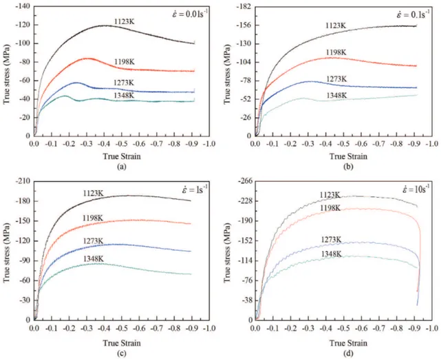
sT is the true stress, sN is the nominal stress, εT is the true strain and εN is the nominal strain1,2. The true compressive stress-strain curves of as-extruded 42CrMo high-strength steel deformed at four temperatures and four strain rates are shown as Figure 2a~d, which in turn would be used to compute the ANN model.
3. Experimental Results
The true compressive stress-strain curves obtained from the hot compression tests of 42CrMo steel are depicted in Figure 2. The flow stress as well as the shape of the flow curves is sensitively dependent on temperature and strain rate. From the stress-strain curves, three types of curve variation tendency can be generalized. Firstly, the exceptional case that the flow stress increases monotonically from beginning to end with significant dynamic work-hardening (WH) (1123 K & 0.1 s–1). The flow stress at temperature of 1123K and strain rate of 0.1 s–1 increases monotonically from beginning to end, which is a special case responding with significant dynamic work-hardening (WH). Such is due to the fact that dislocation multiplication with deformation increasing. Meanwhile, at lower temperature, the flow stress increasing which is attributed to the fact that lower mobilities at boundaries and sliding of dislocation is much difficult; Secondly, the flow stress gradually increases to a peak (initial working hardening) and then decreases slowly to a steady state indicating DRX softening (1123~1348 K & 0.01 s–1, 1198~1348 K & 0.1 s–1, 1273~1348 K & 1 s–1); Thirdly, the flow stress curves have no apparent peak stress with the softening mechanism dynamic recovery (DRV)
characterizing (1123~1198 K & 1 s–1, 1123~1348 K & 10 s–1). Therefore, the analysis of true compressive stress-strain curves reveals that the hot deformation behavior of 42CrMo steel is very complex and highly nonlinear with various metallurgical phenomena like work hardening, dynamic recovery and dynamic recrystallization.
4. Development of the ANN Model for
42CrMo Steel
4.1.
Artificial neural model
Artificial neural network (ANN) is a relatively new artificial intelligence technique that emulates the behavior of biological neural systems in digital software or hardware. The ANN model consists of an interconnected group of processing elements which are called artificial neurons. Some neurons receiving input signals were called the input layer; while other neurons generating output signals were called the output layer. Besides, rest of the neurons as the hidden layers to mimic the complex nonlinear relationships between input signals and output signals. In this study, a multilayer neural network based feed-forward network with back-propagation (BP) algorithm has been adopted, since
the multilayer neural network is a quite efficient tool to understand, memorise and generalize the highly nonlinear characteristics. A typical ANN model consists of an input layer, one or more hidden layers and one output layer. The ANN model can learn from examples and recognize patterns in a series of input and output data using the back-propagation learning algorithm. BP algorithm learns the constitutive relationships between the selected inputs and outputs, and it adjusts the weights and biases to minimize the target error by utilizing gradient descent during training procedure. Hence, a feed forward network trained with the back propagation algorithm was developed, as shown in Figure 3.
In the ANN model, the input variables are deformation temperature (T), strain rate (ε) and strain (ε), while the output variable is flow stress (s). The experimental data (total of 720 experimental data points) obtained from the compression test were used to train and test the model. All the data were divided into two sets: 82% data points were selected as training dataset for training the ANN model and the remaining 18% data points (as shown in Table 1) were used as testing dataset for evaluating the performance of the ANN model. As can be seen, the input strain was varies from 0.02 to 0.9 (interval 0.02), the temperature was varies from 1123 K to1348 K and the strain rate was varies from 0.01 to 10 s–1. The output flow stress was varies from 3.86 Mpa to 237.53 Mpa. Therefore, the input and output data were measured in different units, before training, all the data need to be normalized into the dimensionless units to remove the arbitrary effect of similarity between the different data28,29. The temperature, strain and flow stress were normalized within the range from 0 to 0.25 using the relation given by Equation 1, the strain rate was normalized within the range from 0.05 to 0.3 using the relation given by Equation 2.
min n max min 0.95 0.25 * 1.05 0.95 x x x x x
-= - (1)
min n
max min
0.95 0.05 0.25 *
1.05 0.95
x x
x
x x
= + - - (2)
where xn is the normalized value of x, x is the experimental data, xmax and xmin are the maximum and minimum value of
x respectively.
As stated above, the optimal configuration of the ANN model structure should be adopted ensuring a high training accuracy. Architecture selection requires choosing
an appropriate transfer function, training function and an appropriate neuron number for each hidden layer26,27. In the present model, two hidden layers are adopted, the transfer function is determined as ‘tan sigmoid’ for each hidden layer, ‘pure linear’ for output layer30. In order to improve network generalization ability, the ANN model was optimized by the training function with neural network optimization algorithms. ‘Trainbr’ is a network training function that updates the weight and bias values according to Levenberg-Marquardt optimization. It minimizes a combination of squared errors and weights, and then determines the correct combination so as to produce a network that generalizes well. The process is called Bayesian regularization method. The method involves modifying the performance function by adding a term that consists of the mean of the sum of squares of the network weights and biases (msereg), which was shown in Equation 3. Using this performance function causes the network to have smaller weights and biases, and it forces the network response to be smoother and less likely to overfit.
(
) ( )
1 2 2
2 1 1 1 2 1 1 1 n n
i i j
i j
msereg t a
n == n
= g ⋅ ⋅∑ - + - g ⋅ ⋅ ω∑ (3)
Where g is the performance ratio, ti is the target value,
ai is the output value, n1 is the number of training sample,
n2 is the number of network weights.
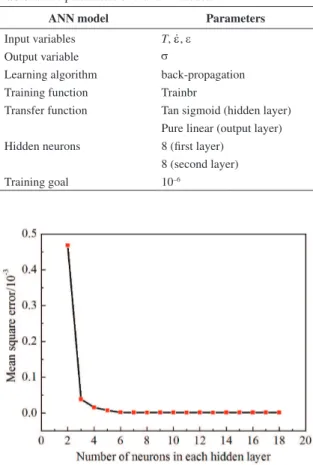
The neuron number for each hidden layer is often settled by a trail-and-error procedure according to the experience of designers. If the neuron number of each hidden layer in the ANN model is too much, the neural network would be complex and too more neurons may slow the convergence rates or overfit the data. Otherwise, the trained network may not learn the process sufficiently. The value of mean square error (MSE) obtained from Equation 4 is used to check the ability of the trained network.
(
)
2 11 N
i i
i
MSE E P
N =
= ∑ - (4)
Where E is the sample of experimental value, P is the sample of predicted value by ANN model, N is the number of strain-stress samples.
As a series of ANN models with different neuron number had been trained well, the MSE values which show the influence of neuron number for each hidden layer on the network performance were calculated. As shown in Figure 4, the mean square error (MSE) is relatively constant with the increasing of neuron number; it indicates that the algorithm has converged. It can be seen that the MSE value decreases to the minimum value when the neuron number was increased to eight in each hidden layer, respectively. It indicates that the ANN model with eight neurons in each hidden layer provides the best performance.
4.2.
The evaluation of the ANN model
The ANN model for predicting the flow stress of 42CrMo steel was developed by the unified training datasets corresponding to true strains of 0.02~0.9, temperatures of 1123 K, 1198 K, 1273 K, 1348 K, and strain rates of 0.01 s–1, 0.1 s–1, 1 s–1, 10 s–1 respectively. Table 1 shows
the experimental and predicted flow stress along with the associated absolute error and relative percentage error for the testing data. The absolute error is the deviation between the predicted and experimental values which expressed by Equation 5. The relative percentage error is introduced which expressed by Equation 6. Relative percentage error is used to compare different measurements because, being a percent, it compare each error in terms of 100.
= i i
Absolute err Eor -P (5)
( )
% = i i 100%i
Relative r E P E
erro - × (6)
where E is the sample of experimental value, P is the sample of predicted value by one model, N is the number of strain-stress samples.
It is found that the absolute error obtained from ANN model varies from –3.69 to 3.67 (Mpa), whereas the relative percentage error is in the range from –5.72% to 4.45%. As shown in Figure 5a, the absolute errors are within ±4 (Mpa), the maximum absolute error between the predicted and experimental values is 3.69 (Mpa). As shown in Figure 5b, the relative percentage errors are within ±6%, the maximum relative percentage error between the predicted and experimental values is 5.72%, which reveals the high accuracy of the developed ANN model. In addition, in order to evaluate the predictability of the ANN model, two evaluators, correlation coefficient (R) and average absolute relative error (AARE) are introduced, and it is expressed by Equation 7 and Equation 8, respectively. R is commonly used to represent the strength of linear relationship between experimental values and predicted values. AARE is very similar to the relative squared error in the sense that it is also relative to a simple predictor, which is just the average of the actual values. In this case, though, the error is just the total absolute error instead of the total squared error. Thus, the relative absolute error takes the total absolute error and normalizes it by dividing by the total number of strain-stress samples.
2 2
1
)( )
) ( )
N
i i
i 1
N N
i i
i 1 i
(E E P P R
(E E P P
=
==
-
-=
-
-∑
∑ ∑ (7)
1
(%) 100
N
i i
i i
E P 1 AARE
N = E
-=× ∑ (8)
where E is the sample of experimental value, P is the sample of predicted value by ANN model, E and P are the mean value of E and P respectively, N is the number of strain-stress samples.
Table 1. The parameters of the ANN model.
ANN model Parameters
Input variables T, ε, ε
Output variable s
Learning algorithm back-propagation
Training function Trainbr
Transfer function Tan sigmoid (hidden layer)
Pure linear (output layer)
Hidden neurons 8 (first layer)
8 (second layer)
Training goal 10–6
Figure 4. The influence of neuron number for each hidden layer on the network performance.
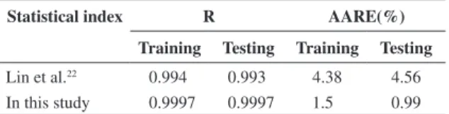
Comparisons of the ANN predicted flow stress with the experimental flow stress during training and testing are shown in Figure 6a and b respectively. Table 2 shows the
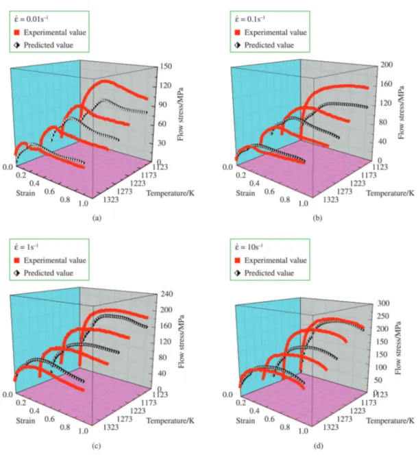
R-values and AARE-values of the ANN models constructed by Lin et al.22 and in this study respectively. It can be seen that the higher R-value and lower AARE-value were obtained from the ANN model constructed in this study. Observations indicate the developed ANN model for 42CrMo steel has good prediction ability. After the ANN model is evaluated, the predicted flow stress from the ANN model and the corresponding experimental flow stress at different deformation temperatures and strain rates were compared. As shown in Figure 7, the constitutive data predicted by the ANN model are fit with the experimental results well not only at the hardening stage but also at softening stage (whatever it is DRX or DRV softening mechanism). Therefore, it can be concluded that the ANN model is an effective tool to predict the complex nonlinear high temperature deformation behavior of 42CrMo steel.
5. The Application of ANN Model in
Isothermal Compression Deformation
5.1.
Prediction potentiality of the ANN model
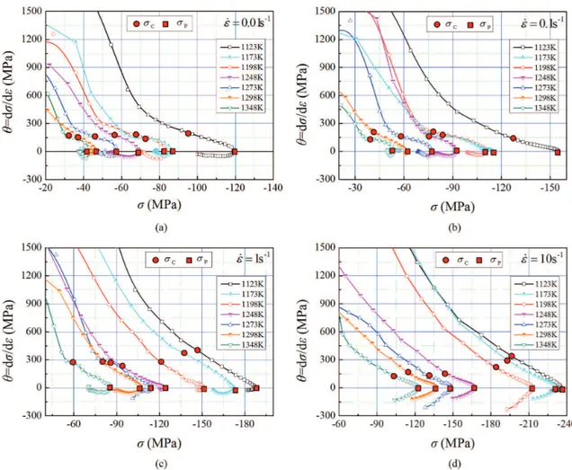
The developed ANN model is applied to simulate the deformation behavior of 42CrMo steel. For obtaining more constitutive information of 42CrMo steel, the developed ANN model was extended to predict the constitutive data at supposed temperatures of 1173K, 1248 K, 1298 K and strain rates of 0.01 s–1, 0.1 s–1, 1 s–1, 10 s–1, which were not included in the compression tests. The constitutive data are shown in Figure 8a~d, in which each solid line represents
the 3D response plot of experimental stresses to strain and temperature under a fixed strain rate, meanwhile each dash line composed of a rhombus matrix represents the 3D response plot of predicted stresses outside of experimental conditions. As expected, the obtained constitutive data from the ANN model show the same variation with temperature, strain rate and strain as experimental data. From the predicted stress-strain curves, it can be concluded that the work-hardening effect is pronounced at higher strain rate and lower temperature. For the higher temperature and lower strain rate, the stress-strain curves show transient flow softening behavior. Here, the experimental and the predicted stress-strain data (Figure 8a~d) was analyzed by fitting each curve with a polynomial expression and taking its derivative with respect to strain in order to obtain the work hardening rate. As shown in Figure 9a~d, the WH rate (q = ds/dε) is the derivative of stress with respect to strain (ε), which corresponds to the tangent at this value of strain. The q – s curves outside of experimental conditions, as well as the q – s curves under experimental conditions, gradually decrease to a lower slope and then drop towards
q = 0 at peak stress, sP, from the inflection at critical stress,
sC indicating the occurrence of DRX.
It can be seen that the predicted stress evolution with strain exhibits three types of curve variation tendency. Firstly, the exceptional case that the flow stress increases monotonically from beginning to end showing dynamic work-hardening (WH) (1173 K & 0.1 s–1); Secondly, the flow stress decreases gradually to a steady state indicating DRX softening (1173~1298 K & 0.01 s–1, 1248~1298 K & 0.1 s–1, 1173~1298 K & 1 s–1); Thirdly, the flow stress maintains a steady state flow with higher stress level with the softening mechanism DRV characterizing without significant softening and work-hardening (1173~1298 K & 10 s–1). It can be summarized that the typical form of flow curve with DRX softening, including a single peak followed by a steady state flow as a plateau, is more recognizable at high temperatures and low strain rates. It is found that the predicted stress-strain curves outside the experimental conditions articulate the similar relationships with experimental stress-strain curves. Therefore, it can conclude that the developed ANN model has good prediction
Table 2. Comparison between the models constructed by
Lin et al.22 and in this study.
Statistical index R AARE(%)
Training Testing Training Testing
Lin et al.22 0.994 0.993 4.38 4.56
In this study 0.9997 0.9997 1.5 0.99
potentiality to predict the highly nonlinear deformation behavior.
5.2.
Model application in isothermal
compression deformation
In this section, the predicted constitutive data were used as the basic data in the finite element method (FEM) analysis software DEFORM-2D. To evaluate the accuracy of the constitutive data obtained by ANN model, the hot compression simulations at the deformation temperature of 1273 K and strain rate of 0.01~10 s–1, as a comparison, was performed. The meshed finite element model for initial billet is shown in Figure 10a. The dimensions of the initial billet are diameter 10mm and height 12mm. The deformed block with deformation degree of 60% (reduction in height) is shown in Figure 10b. According to the lubricated conditions that graphite lubricants were used to coat the top and bottom surfaces of specimen during compression test, the friction at the deformed block-tooling interfaces was assumed to be of shear type and friction factor was assumed to be 0.3. In order to approximate the actual condition of hot isothermal compression test, thermal radiation and heat exchange between billet, dies and surrounding atmosphere were ignored.
During the simulation, the billet was deformed at the constant strain rate of 0.01~10 s–1, the bottom die was set to be the fixed, the movement of the top die was set by displacement control mode according to the Equation 9:
(
)
0 1 exp( )
L=L - -εt (9)
Where, L is the compression amount of workpiece, which also equates with the displacement of the top die, while L0 is the original height of workpiece. ε is the expected constant strain rate in the heart of workpiece under the above displacement control mode. t is the corresponding compression time at the compression amount of L.
During isothermal compression tests, the load-stroke data of 42CrMo steel were recorded by the Gleeble-1500 thermal-mechanical simulator. Therefore, the forming loads (1273 K & 0.01s–1~10s–1) which were acquired using the load-stroke data obtained from the isothermal compression tests were used as the experimental values. However, when the experimental material data (1123 K, 1198 K, 1348 K & 0.01s–1~10s–1) were used as the constitutive data in the FEM simulation process, the forming load (1273 K & 0.01s–1~10s–1) obtained from the FEM simulation results were used as the validation values. While when the experimental material data (1123 K, 1198
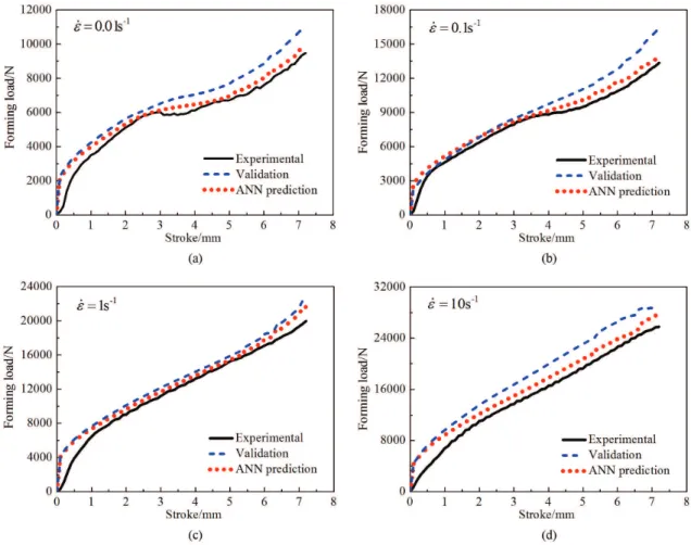
K, 1348 K & 0.01s–1~10s–1) and the ANN predicted data (1173 K, 1248 K, 1298 K & 0.01s–1~10s–1) were used as the constitutive data in the FEM simulation process, the forming load (1273 K & 0.01s–1~10s–1) obtained from the FEM simulation results were used as the predicted values. The experimental and simulation results were shown in Figure 11. Basically, the constitutive data which were used in the simulation are discontinuous, the simulation process was conducted through interpolation method. Therefore, when the ANN predicted constitutive data were applied in the FEM simulation, it is found that the predicted values can well track the upsetting experiment results on thermal physics simulator Gleeble-1500. As shown in Figure 12, the maximum forming load relative errors between the experimental results and the FEM simulation results are introduced which expressed by Equation 5, during which
E is the sample of experimental value, P is the sample of
validation values or the ANN predicted value respectively. The validation relative errors between the validation values and experimental values with the deformation degree of 60% are found to be –18.06%, –23.30%, –12.51%, –13.07% under the strain rates of 0.01 s–1, 0.1 s–1, 1 s–1, 10 s–1 respectively. While the predicted relative errors between the predicted values and experimental values with the deformation degree of 60% are found to be –4.82%, –3.92%, –8.48%, –7.95% under the strain rates of 0.01 s–1, 0.1 s–1, 1 s–1, 10 s–1 respectively. The results show that the predicted data obtained by ANN model outside the experimental conditions successfully improved the prediction accuracy of the forming load in the FEM simulation. Therefore, it can concluded that the predicted data obtained by ANN model outside the experimental conditions are effective and helpful for FEM simulation.
Figure 9. q = ds/dε versus plots under different deformation temperatures with strain rates (a) 0.01 s–1, (b) 0.1 s–1, (c) 1 s–1, (d) 10 s–1.
5.3.
Microstructural evolution
Optical microstructures of 42CrMo high-strength steel at a fix true strain of 0.9, a fix temperature of 1273 K and different strain rates were shown in Figure 13. It found that the initial equiaxed grains (as shown in Figure 1) with a
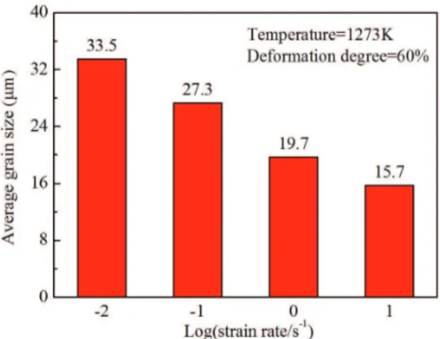
large quantity of twin boundaries transform to recrystallized grains with wavy or corrugated grain boundaries. In fact, the dislocation density tends to accumulate as the strain rate increase thereby the flow stress increases and the DRX softening decreases correspondingly. Therefore, the forming load increases with the increase of strain rate due to the fact that the stress increase with the increase of strain rate, which in turn requires large forming load. Furthermore, in Figure 14, as deformation strain rate (in log scale) increases, the initial microstructure with average grain size of 53.1µm becomes more and more refined due to the fact that there is no enough time for DRX.
6. Conclusions
The constitutive relationship of 42CrMo steel was established using the ANN model, the optimal architecture of ANN model is 3-8-8-1, the inputs are deformation temperature, strain rate and strain, whereas flow stress is the output. The conclusions are as following:
(1) The R-value and AARE-value for the training data are found to be 0.9997 and 1.50% respectively, meanwhile, the R-value and AARE-value for the testing data are found to be 0.9997 and 0.99% respectively, indicating that the ANN model has higher predictability.
Figure 11. Comparisons among validation, ANN prediction and experimental values with deformation degree of 60% and strain rates (a) 0.01 s–1, (b) 0.1 s–1, (c) 1 s–1, (d) 10 s–1.
Figure 13. Optical microstructures of as-extruded 42CrMo high-strength steel at a fix true strain of 0.9, a fix temperature of 1273 K and different strain rates: (a) 0.01 s–1, (b) 0.1 s–1, (c) 1 s–1, (d) 10 s–1.
Figure 14. Average grain size of 42CrMo high-strength steel at a fix temperature of 1273 K and different strain rates.
(2) The predicted stress-strain curves outside the experimental conditions articulate the similar relationships with experimental stress-strain curves. Meanwhile, the q – s curves indicate that the predicted constitutive data exhibit a typical dynamic recrystallization softening characteristic of high temperature deformation behavior.
(3) The predicted constitutive data outside the experimental conditions successfully improved the prediction accuracy of forming load in the FEM simulation. It is found that the ANN model is an effective tool which was applied in the FEM simulation.
Acknowledgements
References
1. Quan GZ, Tong Y, Luo G. and Zhou J. A characterization for the flow behavior of 42CrMo steel [J]. Computational Materials Science. 2010; 50(1):167-171. http://dx.doi.org/10.1016/j. commatsci.2010.07.021
2. Lin YC, Chen MS and Zheng J. Microstructural evolution in 42CrMo steel during compression at elevated temperatures [J]. Materials Letters. 2008; 62(14):2132-2135. http://dx.doi. org/10.1016/j.matlet.2007.11.032
3. Quan GZ, Li GS, Chen T, Wang YX, Zhang YW and Zhou J. Dynamic recrystallization kinetics of 42CrMo steel during compression at different temperatures and strain rates [J].
Materials Science and Engineering: A. 2011; 528(13-14):4643-4651. http://dx.doi.org/10.1016/j.msea.2011.02.090
4. Chen MS and Lin XS. The kinetics of dynamic recrystallization of 42CrMo steel [J]. Materials Science and Engineering: A. 2012; 556:260-266. http://dx.doi.org/10.1016/j. msea.2012.06.084
5. Haghdadi N, Zarei-Hanzaki A and Abedi HR. The flow behavior modeling of cast A356 aluminum alloy at elevated temperatures considering the effect of strain [J]. Materials Science and Engineering: A. 2012; 535:252-257. http://dx.doi. org/10.1016/j.msea.2011.12.076
6. Marandi A, Zarei-Hanzaki A, Haghdadi N and Eskandari M. The prediction of hot deformation behavior in Fe–21Mn– 2.5Si–1.5Al transformation-twinning induced plasticity steel [J]. Materials Science and Engineering: A. 2012; 554:72-78. http://dx.doi.org/10.1016/j.msea.2012.06.014
7. Zhang HJ, Wen WD, Cui HT and Xu Y. A modified Zerilli–Armstrong model for alloy IC10 over a wide range of temperatures and strain rates[J]. Materials Science and Engineering: A. 2009; 527:328-333. http://dx.doi. org/10.1016/j.msea.2009.08.008
8. Voyiadjis GZ and Almasri AH. A physically based constitutive model for fcc metals with applications to dynamic hardness[J].
Mechanics of Materials. 2008; 40: 549-563. http://dx.doi. org/10.1016/j.mechmat.2007.11.008
9. Lin YC and Chen XM. A critical review of experimental results and constitutive descriptions for metals and alloys in hot working [J]. Materials & Design. 2011; 32(4):1733-1759. http://dx.doi.org/10.1016/j.matdes.2010.11.048
10. Ji GL, Li FG, Li QH, Li HQ and Li Z. A comparative study on Arrhenius-type constitutive model and artificial neural network model to predict high-temperature deformation behaviour in Aermet100 steel [J]. Materials Science and Engineering: A. 2011; 528(13-14):4774-4782. http://dx.doi.org/10.1016/j. msea.2011.03.017
11. Serajzadeh S. Prediction of thermo-mechanical behavior during hot upsetting using neural networks [J]. Materials Science and Engineering: A. 2008; 472(1-2):140-147. http://dx.doi. org/10.1016/j.msea.2007.03.037
12. Phaniraj MP and Lahiri AK. The applicability of neural network model to predict flow stress for carbon steels [J]. Journal of Materials Processing Technology. 2003; 141(2):219-227. http://dx.doi.org/10.1016/S0924-0136(02)01123-8
13. Ramanujam J and Sadayappan P. Mapping combinatorial optimization problems onto neural networks[J]. Information Sciences. 1995, 82(3):239-255. http://dx.doi.org/10.1016/0020-0255(94)00052-D
14. Wu W, Dandy GC and Maier HR. Protocol for developing ANN models and its application to the assessment of the quality of the ANN model development process in drinking water quality
modelling[J]. Environmental Modelling & Software. 2014; 54:108-127. http://dx.doi.org/10.1016/j.envsoft.2013.12.016
15. Werbos PJ. Backpropagation through time: what it does and how to do it[J]. Proceedings of the IEEE. 1990; 78(10):1550-1560. http://dx.doi.org/10.1109/5.58337
16. Lu ZL, Pan QL, Liu XY, Qin YJ, He YB and Cao S. Artificial neural network prediction to the hot compressive deformation behavior of Al–Cu–Mg–Ag heat-resistant aluminum alloy [J].
Mechanics Research Communications. 2011; 38(3):192-197. http://dx.doi.org/10.1016/j.mechrescom.2011.02.015
17. Li HY, Li DD, Li YH and Wang XF. Application of artificial neural network and constitutive equations to describe the hot compressive behavior of 28CrMnMoV steel [J]. Materials & Design. 2012; 35:557-562. http://dx.doi.org/10.1016/j. matdes.2011.08.049
18. Ji GL, Li FG, Li QH, Li HQ and Li Z. Prediction of the hot deformation behavior for Aermet100 steel using an artificial neural network [J]. Computational Materials Science. 2010; 48(3):626-632. http://dx.doi.org/10.1016/j. commatsci.2010.02.031
19. Zhu YC, Zeng WD, Sun Y, Feng F and Zhou YG. Artificial neural network approach to predict the flow stress in the isothermal compression of as-cast TC21 titanium alloy [J].
Computational Materials Science. 2011; 50(5):1785-1790. http://dx.doi.org/10.1016/j.commatsci.2011.01.015
20. Sabokpa O, Zarei-Hanzaki A, Abedi HR and Haghdadi N. Artificial neural network modeling to predict the high temperature flow behavior of an AZ81 magnesium alloy [J]. Materials & Design. 2012; 39:390-396. http://dx.doi. org/10.1016/j.matdes.2012.03.002
21. Haghdadi N, Zarei-Hanzaki A, Khalesian AR and Abedi HR. Artificial neural network modeling to predict the hot deformation behavior of an A356 aluminum alloy [J]. Materials Science and Engineering: A. 2013; 49:386-391.
22. Lin YC, Zhang J and Zhong J. Application of neural networks to predict the elevated temperature flow behavior of a low alloy steel [J]. Computational Materials Science. 2008; 43(4):752-758. http://dx.doi.org/10.1016/j.commatsci.2008.01.039 23. Sheikh H. and Serajzadeh S. Estimation of flow stress behavior
of AA5083 using artificial neural networks with regard to dynamic strain ageing effect [J]. Journal of Materials Processing Technology. 2008; 196(1-3):115-119. http://dx.doi. org/10.1016/j.jmatprotec.2007.05.027
24. He YB, Pan QL, Chen Q, Zhang ZY, Liu XY and Li WB. Modeling of strain hardening and dynamic recrystallization of ZK60 magnesium alloy during hot deformation [J].
Transactions of Nonferrous Metals Society of China. 2012; 22(2):246-254. http://dx.doi.org/10.1016/S1003-6326(11)61167-9
25. Hecht-Nielsen R. Theory of the backpropagation neural network [J]. International Joint Conference on. 1989:593-605.
26. Reddy NS, Lee YH, Park CH and Lee CS. Prediction of flow stress in Ti–6Al–4V alloy with an equiaxed microstructure by artificial neural networks [J]. Materials Science and Engineering: A. 2008; 492:276-282. http://dx.doi. org/10.1016/j.msea.2008.03.030
27. Quan GZ, Lv WQ, Mao YP, Zhang YW and Zhou J. Prediction of flow stress in a wide temperature range involving phase transformation for as-cast Ti–6Al–2Zr–1Mo–1V alloy by artificial neural network[J]. Materials Science and Engineering: A. 2013; 50:51-61.
hot torsion [J]. Applied Soft Computing. 2009; 9(1):237-244. http://dx.doi.org/10.1016/j.asoc.2008.03.016
29. Li HY, Wang XF, Wei DD, Hu JD and Li YH. A comparative study on modified Zerilli–Armstrong, Arrhenius-type and artificial neural network models to predict high-temperature deformation behavior in T24 steel. Materials Science
and Engineering: A. 2012; 536:216-222. http://dx.doi. org/10.1016/j.msea.2011.12.108
30. Holthausen K and Breidbach O. Analytical description of the evolution of neural networks: learning rules and complexity[J].