Implementation of multiple 3D scans for error calculation on object digital reconstruction

Implementation of multiple 3D scans for error calculation on

object digital reconstruction

Sidiropoulos Andreas*, Lakakis Konstantinos**

*Department of Civil Engineering, Aristotle University of Thessaloniki, Greece

ABSTRACT

Laser scanning is a widespread methodology of visualizing the natural environment and the manmade structures that exist in it. Laser scanners accomplish to digitalize our reality by making highly acc urate measurements. Using these measurements they create a set of points in 3D space which is called point cloud and depicts an entire area or object or parts of them. Triangulation laser scanners use the triangle theories and they main ly are used to visualize handheld objects at a very close range fro m them. In many cases, users of such devices take for granted the accuracy specifications provided by laser scanner manufacturers and respective software and for many applications this is enough. In this paper we use point clouds, collected by a triangulation laser scanner under a repetition method, of two cubes that are geometrically similar to each other but differ in material. At first, the data of each repetition are being compared to each other to examine the consistency of the scanner under multip le measurements of the same scene. Then, the reconstruction of the objects‟ geometry is achieved and the results are being compared to the data derived by a digital caliper. The errors of calcu lated dimensions were estimated by the use of error propagation law.

Keywords:

I.

INTRODUCTION

Laser scanners measure very dense point clouds in a very short period of time. The data consist of thousands, millions or even billions of points that the user must process and extract only the useful information. In this paper we use the measurements on two geometrically similar objects, acquired by a triangulation laser scanner, to digitally reconstruct their geometry. In most cases of geometric docu mentation the data that a laser scanner captures after one measurement are considered reliable for the purpose of the application they are being used. In the current case, we do not make measurements of the objects of interest just once. We use multip le measurements so we can assess the reliability of the scanner in data collection. The objects that were used are two cubes of theoretically same dimensions that differ in material and color. The first one is wooden and the second is metallic. Each measurement was made ten times and each time the scene was remained exactly the same. In this way we collected the data that would be used to examine the reliability of the scanner on repeating the exactly same measurement. Ne xt, we used the data derived by the multiple scans to calculate the errors of the objects‟ vertices coordinates and we implemented the error propagation law to estimate the errors of the calculated edges. The final dimensions that were extracted using the multiple 3D scans were compared to the measurements that were made by the use of a digital caliper.

The technique of measurements under

applications. Especially for total stations and GPS, repetitions are mandatory for acquiring more reliable and accurate results. Concerning laser scanners, repetition is not widely used. A very common case is to compare data collected from the same scene at different time mo ments to detect differences and changes but the case of measuring the exact same scene more than once to evaluate the scanner as a metric device is not that common. Efforts to this direction are very welcomed, because there is no much information available to the users for the accuracy and reliability of such instruments. An important experiment to investigate the laser scanner accuracy was made by [1]. The authors tested different laser scanning systems to evaluate their range, angle accuracy and the errors that occur because of different construction material and the different shape of the objects and finally, the errors that are being produced at the edges of the objects. The authors concluded that laser scanners show considerable errors under certain conditions even for applications that accuracy is not that important. The results of the project were availab le to the manufacturers so they can compare the performance of their instrument to other devices and also, the publication of the project can aid users to select the most suitable equipment for their applications. A low-cost triangulation laser scanner was tested by [2] for its evaluation of uncertainty and repeatability. The authors used a wooden birdhouse and scanned it 20 times in macro and 20 times in wide mode that are being provided as

data were compared to the data collected by the use of a caliper and the repeated scans were co mpared to each other. The results for the uncertainty evaluation are ±0.81 mm in macro and ±1.66 mm in wide mode. Repeatability evaluation resulted in ±0.84 mm in macro and ±1.82 mm in wide mode. Finally, authors in [3] presented an analysis of the positional errors of terrestrial laser scanning (TLS) using spherical statistics. As they claim, they preferred spherical statistics because of the 3D vectorial nature of the spatial error and they highlight that their project did not focus on the error sources of TLS but on the advantages of the spherical graphics and statistical analysis over conventional analysis.

II.

Materials and methods

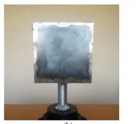
In this paper we make use of repeated scans made by a triangulation laser scanner to accurately reconstruct geometry of two objects. The objects are two theoretically same in geo metry cubes that differ in color and material. Their sides‟ nominal dimensions are 120 mm, one of them is wooden light colored and the other is metallic dark colored. Coded names were given to the cubes so as it is easier to refer to them. The wooden cube was named as the „B‟ object and the metallic as the „G‟ object. Each one of their side was coded using a number and their edges were named by the pair of sides which create them as their intersection. So, object „B‟ contains the sides B1 to B6 and the edges B1-B2, B2-B3 and so on. Coding object „G‟ followed the same rules. The side number 5 corresponds to the top side of the object, number 6 to the bottom and sides 1-4 to the remain ing sides for both objects (Fig. 1).

The structure of the paper is being divided into two main sections. At first we make use of the data measured under repetition and describe the relation among them using as metrics the coordinates of characteristic points of the objects. The second section of this paper focuses on the calculation of the objects‟ edges accompanied by their errors which were estimated using the error propagation law. The final calculated dimensions are being co mpared to the measurements of a digital caliper (±0.01 mm measurement accuracy) which are being considered as the „real‟ dimensions of the objects.

(a)

(b)

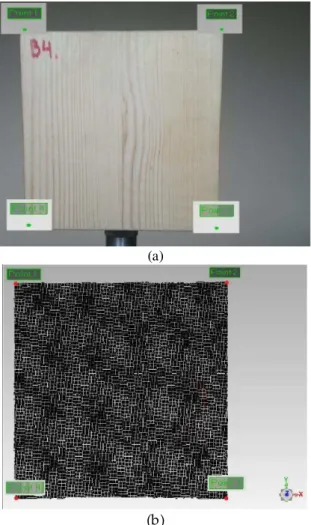
Figure 1. The two objects of edge dimension 120mm: (a) Cube „B‟ (side 1); (b) Cube „G‟ (side

1).

2.1. Data ac quisition

As mentioned previously, the data were collected using two different methods and thus they are being divided into two sets: the „real‟ data and the „test‟ data. The „real‟ data are the measurements made using the digital caliper and the „test‟ data are the repeated scans made by the triangulation laser scanner. The dimensions of the objects were measured thirty times using the digital caliper in order to acquire as accurate as possible value for each one of them.

The „test‟ data were collected by the triangulation laser scanner NextEngine in Wide Mode. This type of laser scanner provides two modes of measuring. The first one is called Macro Mode with a limited field of view (~129x97 mm) and the second is called Wide Mode (343x257 mm) [4]. Because of the fact that we wanted to measure each side of our 120 mm cubes at once and we did not want to create overlapped point clouds we used the Wide Mode whose field of view is big enough to include the whole side size of our cubes (Fig. 2).

(b)

Figure 2. Point clouds of the sides: (a) B1; (b) G1 fro m Figure 1. The point clouds present the measurements of first repetition for each side.

As has already been mentioned we made the laser scanning measurements under a repetition method of ten repetitions for each side. At first, we placed the objects on the base provided by the scanner and then we collected data for ten successive times. It is important to notice that there was no movement of the object or the scanner among none of the ten measurements of each side. Both scanner and object remained stable during the whole procedure of measuring the ten repetitions. After the completion of the ten repetitions we turned the objects at an exactly 90o angle rotation using the mechanism of the laser scanner‟s base and we started a new circle of ten measurements for the next side. Continuing to rotate the objects we covered the sides 1-4. There was no need to measure the sides 5-6 because all of the edges could be calculated using the sides 1-4.

2.2. Eval uation of re peatability

Before using the 3D scans to make the reconstruction of the objects we made some tests to evaluate the ability of the scanner to measure the exact same scene from the same view mo re than once. The tests that took place were two and they focused on two different parameters. The first and simp lest test was to compare the number of points that were contained to each one of the point clouds that were collected during the different repetitions. This test does not provide any sophisticated information about the point clouds. It is just a check of the point population among the repetitions of the same measurement.

The second test to evaluate the repeatability of the scanner focused on the coordinates denoted to some characteristic points. If these points are considered as check points it is very important that their coordinates are very close among the ten repetitions. The first check point was calculated as the mean value of the whole point cloud at each repetition. The determination of this point aids to acquire a general conception and

knowledge about the distribution of the points across the point cloud. If there is high consistency to the measurements that are being provided by the scanner, this point‟s coordinates should be very close to each other of the ten repetitions. The rest check points were not calculated but they were located from the graphical presentation of the point clouds using an appropriate software (Fig. 3).

(a)

(b)

Figure 3. The four vertices of side B4: (a) Photograph of side B4 showing the positions of vertices (green dots); (b) Po int cloud (Repetition 1)

and the location of vertices in it (red dots)

These points are the four vertices of the sides at each repetition. The fact that these points are being selected visually leads to a conclusion of how the measurements of the scanner among the repetitions are similar to each other and help the user to define a point accurately without high affection of the user‟s subjectivity. The check on these points dealt with both of their coordinates separately and also, as their 3D distances from their mean values.

2.3. Eval uation of accur ac y

the vertices‟ location and the standard deviations of the mean that each one of their coordinates was calculated gave us the ability to estimate the values of the cubes‟ edges and their respective error. To accomplish that, we imp lemented the error propagation law on the calculation of distance using coordinates [5], [6] (Equation 1):

(1)

where is the 3D distance between point 1 and point 2, x1, y1, z1 are the 3D coordinates of point 1 and x2, y2, z2 are the 3D coord inates of point 2.

The error propagation law indicates that to calculate the error of distance d (σd) we first have to calculate the partial derivatives of Equation 1 according to Equation 2:

(2)

where σx1, σx2, σy1, σy2, σz1, σz2 are the standard deviations of the mean of the points‟ 1 and 2 coordinates.

Breaking Equation 2 in simp lest parts and in 3D space is given by Equation 3 [7]:

(3)

The calculated distances, with their errors, were co mpared to the respective that were measured using the digital caliper. The differences between these two data sets describe the ability of the laser scanner to digitalize objects in 3D space and as it turned out they describe the scanner‟s difficulty to measure objects‟ edges.

III.

RESULTS

The acquisition of the „real‟ dimensions of the cubes was achieved using a digital caliper. The „real‟ dimensions are those values that were compared to the dimensions extracted by the measurements of the scanner and aided in their evaluation.

Table 1 shows the „real‟ values of two of

the objects‟ dimensions with their standard

deviations of the mean. The measurements were made using the same caliper across the whole procedure and by the same user.

Table 1. The values of two „real‟ dimensions for objects „B‟ and „G‟ with their standard deviations

of the mean.

Side ‘Real’ value (mm)

St. De v. of the Mean (mm)

B2-B6 120.06 0.01

B1-B4 119.35 0.01

G1-G6 119.13 0.01

G1-G4 119.54 0.00

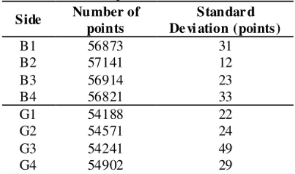
The term repeatability refers to the ability of the scanner to measure the same points and locate them at the same positions among mu ltiple measurements of the same unchangeable and stable scene. It is important to comment that during the ten repetitions that we made for each side of our objects neither the object nor the scanner was moved. The first test that was made to check the repeatability was to count the points of each repetition‟s point cloud and find the differences among them. The point clouds of object „B‟ numbered around 57000 points and the respective of object „G‟ more than 54000. Table 2 shows the mean value of the points‟ number for each object‟s sides and the respective standard deviation, all rounded to the integer unit.

Table 2. Mean number of points for each object‟s sides and the respective standard deviations

Side Number of points

Standar d De vi ation (points)

B1 56873 31

B2 57141 12

B3 56914 23

B4 56821 33

G1 54188 22

G2 54571 24

G3 54241 49

G4 54902 29

It is obvious that the number of points that are being captured during the measurements is very close among the ten repetitions. This test does not provide any statistical analysis for the level of the scanner‟s repeatability but it is an indication of the low randomness among multip le measurements of the exact same scene.

made during the second part of the second test which includes the localization of the vertices of our objects (check points).

The calculation of the mean points for each side and for the ten repetitions gave very satisfying results close to 0.01 mm. Fo r object B the maximu m standard deviation of the mean was calculated for the B4 and for the x-coordinate and its value was ~0.02 mm. The min imu m standard deviation of the mean was that of the side‟s B4 y -coordinate and its value was ~0.01 mm. The maximu m and minimu m standard deviations of the mean for the distances among the mean points of the cube B were ~0.01 mm (side B3) and ~0.00 mm (side B1). For object G the maximu m standard deviation of the mean was found for the side G3 (x-coordinate) and its value was ~0.02 mm and the minimu m was found for the side G4 (z-coordinate) and its value was ~0.00 mm. The distances maximu m standard deviation of the mean among the mean point for cube G was ~0.01 mm (side G3) and the min imu m was ~0.00 mm (side G2).

The test for the remain ing check points (four vertices of each side) required their manually positioning using the graphical environment of a point cloud processing software. We used Geomagic software and we located the cubes‟ vertices at each side and each repetition. In this way we acquired ten sets of data that contain the coordinates of the four vertices. The results of the calculation of the mean values for each vertex using the whole ten repetitions data were very satisfying. Table 3 and Table 4 show the maximu m and minimu m standard deviations of the mean of the vertices of all sides of our objects with respect to their coordinates. Table 5 and Table 6 show the maximu m and minimu m standard deviations of the mean of the vertices‟ distances from their mean value for each vertex.

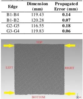
Once we have calculated the coordinates of the four vertices for each side of our objects we were able to calculate the dimensions of their edges and propagating their error (Equation 3) to calculate the dimensions‟ errors based on the observations that made using the multip le point clouds (Table 7). The values of the edges (Equation 1) were co mpared to the respective values that were calculated by the digital caliper. This comparison evaluated the ability of the laser scanner to reconstruct the geometry of objects according to the provided by the manufacturer dimensional accuracy (~0.38 mm) for the Wide Mode. The results are very interesting and can be categorized in two groups. For better understanding, if we consider a rando m side of our objects (Fig. 4) it is obvious that exist four dimensions, two horizontal (top and bottom) and two vertical (left and right). The horizontal distances (intersection of sides 1 to 4 with 5 and 6) have large errors and especially the intersection with side 6 (bottom).

Table 3. Maximu m standard deviations of the mean of objects‟ „B‟ and „G‟ vertices with respect

to their coordinates.

Side Verte x

Coor dinate of max de viation

St. De v. of the Mean

(mm) B1 Point 4 y- 0.11 B2 Point 3 x- 0.10 B3 Point 4 y- 0.09 B4 Point 1 y- 0.10 G1 Point 4 y- 0.10 G2 Point 1 x- 0.17 G3 Point 3 x- 0.15 G4 Point 4 x- 0.11

Table 4. Minimu m standard deviations of the mean of objects‟ „B‟ and „G‟ vertices with respect to their

coordinates.

Side Verte x

Coor dinate of mi n de viation

St. De v. of the Mean

(mm)

B1 Point 3 z- 0.04

B2 Point 4 z- 0.05

B3 Point 2 x- 0.01

B4 Point 4 y- 0.00

G1 Point 3 z- 0.03

G2 Point 3 z- 0.06

G3 Point 1 z- 0.02

G4 Point 1 z- 0.02

Table 5. Maximu m standard deviations of the mean of objects‟ „B‟ and „G‟ vertices with respect

to the distance from their mean value.

Side Verte x of max de viation

St. De v. of the Mean (mm)

B1 Point 1 0.06

B2 Point 1 0.06

B3 Point 2 0.04

B4 Point 1 0.07

G1 Point 4 0.07

G2 Point 4 0.09

G3 Point 3 0.09

G4 Point 4 0.07

Table 6. Minimu m standard deviations of the mean of objects‟ „B‟ and „G‟ vertices with respect to the

distance from their mean value.

Side Verte x of min de viation

St. De v. of the Mean (mm)

B1 Point 4 0.05

B2 Point 4 0.02

B3 Point 1 0.02

B4 Point 2 0.04

G1 Point 3 0.03

G2 Point 2 0.03

G3 Point 1 0.03

Table 7. Dimensions with maximu m and minimu m propagated error for both objects.

Edge Dime nsion (mm)

Propagate d Error (mm) B1-B4 119.43 0.14 B1-B2 120.28 0.07 G2-G5 116.55 0.18 G3-G4 119.83 0.06

Figure 4. A random side of our objects. Top and bottom dimensions tend to shrink the object at the direction that yellow arrows indicate.

Compared to the scanner‟s dimensional accuracy, these errors are more than five times bigger. On the other hand, the accuracy achieved for the vertical dimensions (intersections among sides 1-4) is more satisfying. The errors‟ values are smaller than the scanner‟s dimensional accuracy. The above facts are real for both object „B‟ and

object „G‟. Table 8 shows the maximu m and

minimu m errors calculated by the differences between laser scanning and digital caliper data.

Table 8. Maximu m and minimu m errors between objects‟ „test‟ and „real‟ dimensions.

Edge

‘Test’ di me nsion

(mm)

‘Real’ di me nsion

(mm)

Error (mm)

B1-B5 117.24 120.02 +2.78 B3-B6 116.79 119.75 +3.53 G3-G5 116.01 119.14 +3.13 G3-G6 115.69 119.29 +3.60 B2-B3 119.35 119.27 -0.08 B4-B3 118.80 118.75 -0.05 G2-G3 119.66 119.62 -0.04 G1-G4 119.80 119.54 -0.26

IV.

CONCLUSION

In this paper we used the idea of mu ltiple measurements on 3D laser scanning. The data collection comp leted after a circle of ten repetitions for each side of our two cubes. The aim of this project was twofold. Firstly, we wanted to evaluate the ability of a triangulation laser scanner to repeat the exact same measurement under absolute same conditions. The second goal was to evaluate the reconstruction of objects using the 3D scans

compared to the dimensions provided by a digital caliper.

The errors of point clouds mean points positioning were much lower than the scanner manufacturer suggested accuracy. This fact is very satisfying related to the ability of the scanner to make similar more than one replicates of an object. Also, the errors found for the coordinates of the objects vertices show a very high level of repeatability. On the other hand, the reconstruction accuracy revealed both an advantage and a weakness of the scanner. The disadvantage is that there is a trend of lower accuracy across the x-axis. This axis is the one that the motion of the laser lines is happening during the measurements and there was no good imprint taken by the scanner probably because of the quick passing from the objects‟ edges. In the contrary, the dimensionality accuracy across y-axis (vertical to the movement of laser lines) was better even from this that the manufacturer provided. The errors that were produced by the measurements on both of our objects were of the same magnitude and followed the same rules. The only notable fact is that usually the standard deviations of the mean of the object „B‟ (wooden light colored cube) were slightly better without considering that this was always the rule. Future wo rk will focus on more tests on measurements by laser scanners for various objects and for various distances between object and laser scanner. Because of lack of information provided by manufacturers on laser scanners‟ specifications, it is very important to make efforts towards the evaluation of accuracy and reliability that laser scanners provide. In this way these devices will be more useful for even more sophisticated applications.

ACKNOWLEDGMENTS

We would like to thank the State Scholarship Foundation for the program “IKY FELLOW SHIPS OF EXCELLENCE FOR POSTGRADUATE STUDIES IN GREECE – SIEMENS PROGRAM”.

REFERENCES

[1]. W. Boehler, A. Marbs, Investigating Laser Scanner Accuracy, i3main z. Institute for Spatial Information and Surveying Technology, FH Mainz, Un iversity of Applied Sciences, Main z, Germany

Url:http://hds.leica-geosystems.com/hds/en/Investi

gating_Acurracy_Mintz_White_Paper.pdf (accessed on 24 November 2016).

[3]. A. Cuartero, J. Armesto, P. Garcνa Rodrνguez and P. Arias, Error Analysis of Terrestrial Laser Scanning Data by Means of Spherical Statistics and 3D Graphs. Sensors 2010, 10, 10128–10145.

[4]. NextEngine. Availab le online: http://www.nextengine.co m/ (accessed on 24 November 2016).

[5]. C. D. Ghilani, Adjust ment computations: spatial data analysis (John Wiley & Sons, 2010).

[6]. J. Taylor, Introduction to error analysis, the study of uncertainties in physical measurements. Vo l. 1. 1997.

[7]. B. Keeney, A Guide to Error Propagation.

Available online: